A Model of Frequency Coding in the Central Auditory Nervous System
J
ohan
J
Hanekom
Department of Electrical and Electronic Engineering University of Pretoria
ABSTRACT
A phenomenological model for neural coding in the central auditory system is presented. This model is based on average rate-place codes and the hypothesis is that the rate-rate-place code present in the population of low spontaneous rate nerve fibres is adequate to account for frequency discrimination thresholds across the entire audible frequency range. The activity of a population of nerve fibres in response to an input pure tone is calculated and a neural spike train pattern is generated. An optimal central observer estimates the input frequency from the spike train pattern. The model output is the frequency differ-ence limen at the specific input frequency, determined from the estimated input frequency. It is shown that a rate-place code can account for psychoacoustically observed frequency difference limens. The model also supports the hypothesis that a hu-man listener does not make full use of all the information relevant to frequency that is available in auditory nerve spike trains.
OPSOMMING
'n Fenomenologiese model vir neurale kodering in the sentrale gehoorstelsel word voorgestel. Die model is gebaseer op gemiddelde-tempo plekkodering en die hipotese is dat die tempo-plekkode teenwoordig in die groep lae spontane vuurtempo senuvesels voldoende is om frekwensie-diskriminasiedrempels oor die hele hoorbare frekwensiebereik te verklaar. Die aktiwiteit van 'n populasie van senuweevesels word bereken in reaksie op 'n enkeltoon-inset. 'n Neurale aksiepotensiaalpatroon word hieruit genereer. Die insetfrekwensie word deur 'n optimale sentrale waarnemer geskat vanuit die aksiepotensiaalpatroon: Die modeluitset is die net-waarneembare frekwensieverskil vir die gegewe insetfrekwensie, bepaal uit die geskatte insetfrekwensie. Daar word aangetoon dat 'n tempo-plekkode psigoakoesties-waargenome frekwensie-diskriminasiedrempels kan verklaar. Die model ondersteun ook die hipotese dat mens like luisteraars nie ten volle gebruik maak van al die frekwensie-inligting beskikbaar in die gehoorsenuwee se aksiepotensiaalpatrone nie.
/ ,/
KEY WORDS: rate-place codes, population coding, central auditory system, frequency discrimination, modelling.
INTRODUCTION
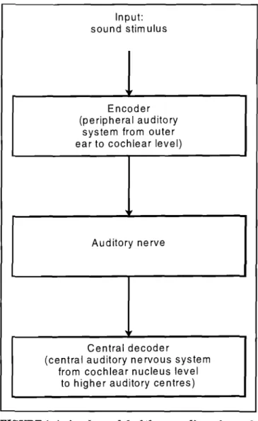
A sound stimulus received by the peripheral auditory system is transformed to neural spike train activity in a population of auditory nerve fibres (called a spike train pattern). The auditory system varies a number of param-eters of the neural spike train pattern to accurately repre-sent a sound, e.g. average spike rate, spread of excitation over a specific subset ofthe neural population and synchro-nization of spikes to the stimulus waveform (Delgutte, 1995). This process of transformation of the original sound stimulus to an internal spike train pattern representation is called coding (Bialek, 1991) and the internal.representa-tion of a stimulus is referred to as the neural code for this stimulus (figure 1). Two mechanisms known to be involved in frequency coding in the auditory system are rate-place coding and phase lock coding (Delgutte, 1997; Moore & Sek, 1996). In rate-place coding, the auditory system may use the excitation pattern across the entire auditory nerve popu-lation to determine the stimulus frequency. Rate-place cod-ing operates over the entire stimulus frequency range, but
is dominant for the coding of high frequencies (above about 5000 Hz) (Kim & Parham, 1991; Moore, 1973). Phase lock coding, i.e., synchronization of neural firing rate to indi-vidual cycles of a periodic stimulus, is the primary cue used for determination of the frequency of a pure tone at low frequencies. Phase locking is progressively lost as stimu-lus frequency increases above about 2500 Hz (Delgutte, 1995). Both coding mechanisms probably operate in paral-lel over a large range of frequencies, but it is not clear yet to which extent the central auditory system uses either mechanism alone or both mechanisms simultaneously in the determination of the frequency ofa pure tone (Johnson, 1980). It is, however, known that at increasingly higher auditory nerve centres more phase-locking is lost and the auditory system relies increasingly on rate-place codes alone (Langner, 1992).
Shofner & Sachs (1986), Kim, Chang & Sirianni (1990) and Kim, Parham, Sirianni & Chang (1991) studied spa-tial response profiles of the discharges of populations of auditory nerve fibres. A "spatial response profile" or "rate response profile" is simply the spatial distribution
ofneu-ce
d
b
y
Sa
bi
ne
t G
at
ew
ay
u
nd
er
li
ce
nc
e
gr
an
te
d
by
th
e
Pu
bl
is
he
r (
d
at
ed
2
01
ral responses (average neural firing rates) to single tone stimuli along the length of the cochlea. An earlier study by Kim and Molnar (1979) indicated that the rate response profiles become very broad and exhibit very little tuning at all but very low stimulation intensities (20 dB SPL). How-ever, they did not clearly distinguish between low sponta-neous rate and high spontasponta-neous rate fibres in their study. Low spontaneous rate (SR) fibres have wider dynamic range (Shofner & Sachs, 1986) and are more likely candidates for rate coding. Shofner and Sachs studied specifically the rate response profiles at low frequency for very low SR fibres (fibres with SR < one spike per second). These fibres ac~
count for about 15% of the afferent auditory nerve popula-tion. Shofner & Sachs found that the rate response profiles for these fibres exhibit clear peaks at the stimulation fre-quency (1500 Hz in their experiments) over a wide range of sound pressure levels (in their experiments, from 34 dB SPL to 87 dB SPL). Kim, Chang and Sirianni (1990) ob-served the same effect with a 1000 Hz stimulus. These
stud-Input: sound stim ulus
,
Encoder (peripheral auditorysystem from outer ear to cochlear level)
Auditory nerve
,.
Central decoder
(central auditory nervous system from cochlear nucleus level
to higher auditory centres)
FIGURE 1. A simple model of the encoding of sound stimuli by the auditory system. The model presented hi ihis article describes the encoding process (which primarily takes place in the cochlea) and the decod-ing process (which takes place in the central audi-tory nervous system at the cochlear nucleus level and higher). The encoder output is the sound stimu-lus encoded as a neural spike train pattern. The decoder output is the estimation of the stimulus parameter, e.g., the frequency of the stimulus.
ies suggested that the rate-place code operates not only at high frequencies, but also over a wide range of sound pres-sure levels at low frequencies.
High SR fibres saturate at relatively low stimulation intensities (Kim, Chang & Sirianni, 1990) and the peak in the excitation pattern at the stimulus frequency is quickly flattened as excitation begins to spread along the length of the cochlea at higher stimulation intensities. Spread of excitation is a cue for loudness (Smith, 1988) and it is there-fore fair to assume (for the purposes of this article) that high SR fibres are primarily involved in intensity coding. Of course, low and high SR fibres are involved in coding of frequency via phase locking as wel1. However, this article focusses on rate coding only and so only low SR fibres are considered.
The articles by Shofner & Sachs (1986), and Kim, Chang
& Sirianni (1990) established that a pure tone stimulus is
represented in the rate code, but it is not actually known whether the rate information is utilized by the central au-ditory system for the extraction of frequency, and if so, how this is achieved. In other words, how does the central audi-tory system go about extracting a single frequency tone from about 28000 (Kim, 1984) nerve fibre spike trains? Of course, the auditory system does not have to extract the tone ex-plicitly, i.e., there need not be an explicit representation of the tone somewhere in the central auditory system. By this it is meant that it is not necessary that the auditory sys-tem has a representation where (for example) only a single neuron fires somewhere in the central auditory system when a 1000 Hz tone at 60 dB SPL is heard. It is, however, known that pure tones are extracted and represented cen-trally in some form, as is demonstrated by (for example) the ability of subjects to discriminate between two frequen-cies and vocalize which was higher in pitch.
This article presents a modelling study and proposes a mechanism for the extraction offrequency information from a population of nerve fibres. This model is phenomenological and does not reveal the complexity of the underlying bio-physical processes. The intention ofthe model is to explain how a tone might be extracted from the activities of a popu-lation of nerve fibres (i.e., the tone is encoded by a popula-tion code), and this is achieved by demonstrating how: we can account for psychophysically observed frequency ~is
crimination difference limens or just noticeable frequency
differences (jndfs). :
Mathematical detail of the numerical model falls outSIde the scope of this article and is not included in the descrip-tion. The philosophy was to elucidate the principles behlnd the model rather than to obscure them with mathematibl
detai1. '
POPULATION CODING
In neural systems (including the auditory system), sen-sory information is represented in the activities of a popula-tion of nerve fibres. Populapopula-tion coding models have been stud-ied before in a more general context of parameter coding by neurophysiological systems (Baldi & Heiligenberg, 1988; Shadlen & Newsome, 1994). In population codip.g systems, input sensory information (in this article, auditory informa-tion in the form' of a single tone) is sanWled.by a limited number of receptors (the inner hair cells in this case). The receptors have rather wide tuning/profiles which overlap considerably. For the tuning profiles of the receptors of the auditory system, see, for example, Kiang (1965) or Ruggero
The South African Journal of Communication Disorders, Vol. 46, 1999
ro
du
ce
d
b
y
Sa
bi
ne
t G
at
ew
ay
u
nd
er
li
ce
nc
e
gr
an
te
d
by
th
e
Pu
bl
is
he
r (
d
at
ed
2
01
85 (1992). Because of the broadness of tuning, a large number
of receptors will be activated by the stimulus. For example, if a listener hears a 1000 Hz pure tone, not only are the fibres that have a characteristic frequency (CF) of 1000 Hz activated, but so are many other fibres with CF in the vicin-ity of 1000 Hz. However, the fibres with CF of 1000 Hz are maximally activated and fibres not tuned to 1000 Hz are activated less strongly. Because the tuning profiles are so wide (see, for example, Johnson, 1980 or Kiang, 1965), even fibres an octave away from the stimulus may be activated, although weakly.
By comparing the relative activity of all the different receptors, an internal picture may be formed by the cen-tral auditory system of the acoustic environment (i.e., the actual physical signal, the pure tone, in this article). Ac-tivities of fibres in the neural population are in the form of trains of action potentials, or spike trains.
In the- model described in this article, the viewpoint of an ideal central observer (Bialek, 1991) is adopted. In other words, the central auditory system is imagined as being a central observer with no knowledge of the "outside world", except that which is reflected by the activity of the popula-tion of auditory nerve fibres. Each nerve fibre forms an in-formation channel.
The central observer is a conceptual model of all the sig-nal processing that takes place in the entire central audi-tory system. It has available an entire population of nerve fibres responding with different activities to the same stimu-lus. The reconstruction of the physical signal by the cen-tral observer can be much more precise than the spacing between adjoining receptors (Snippe& Koenderink, 1992). Just noticeable differences are typically smaller than the tuning widths of the individual receptors.
In the human auditory system, the central observer re-ceives its only image of the acoustic environment by ob-serving spike trains from about 28000 afferent auditory nerve fibres (Kim, 1984; Spoendlin & Schrott, 1989). From these 28000 spike trains, it has to somehow extract the single tone (or tone in noise) which is presented to the lis-tener in a frequency discrimination experiment.
,//
POINT PROCESS DESCRIPTION OF SPIKE TRAINS
The spikes (or action potetialS) of a neural spike train are all very similar in shape ~nd size, but the information-bearing aspect of a spike traih is the times of occurrence of the spikes. Furthermore, spikes are random in the sense that two identical presentations of the same stimulus do not lead to two identical spik~ traIns. Spike trains may dif.; fer in the number of spikes in a given time period and in different times of occurrence of spikes.
Spike trains can be described mathematically as point processes (Johnson, 1996). The theory of point processes describes the occurrence of isolated events (in this case, individual neural spikes) with the mathematical tools of probability theory and statistics. The point process descrip-tion can provide a basis for mathematical analysis of cod-ing of information in spike trains. The point process hav-ing the simplest structure is the Poisson process. Here a Poisson process is a train of spikes, such that the spikes have a Poisson distribution. The Poisson distribution is a mathematical function describing the probability of hav-ing exactly k spikes, placed at entirely random moments, in a time interval T. The Poisson process is characterized by the intensity parameter A. The number of spikes (k) in
, /
an interval T is random, so that the exact number of spikes in the interval T is not known when A is known. However, for larger values of A, a larger number of spikes are ex-pected in the time interval T. The exex-pected number of spikes in an interval T is AT.
Nerve fibres respond to the stimulus by modulating their firing rates (Shadlen & Newsome, 1994). Every nerve fibre shows an increase in discharge rate over a specific range of pure tone frequency, but the spikes are randomly spaced over the duration of the stimulus and repetitions of the same stimulus do not produce the same number of spikes. This suggests that the Poisson distribution provides an adequate description ofthe statistics of neural spike trains on the auditory nerve (Keidel, Kallert & Korth, 1983; Shadlen & Newsome, 1994). After the occurrence of a spike, there is a short period (the refractory period) during which the nerve fibre is unable to produce another spike. The Poisson process disregards refractory effects (Johnson & Swami, 1983) and is therefore not an entirely accurate model for neural spike trains. However, it was chosen for use in the model described in this article, as it is easy to manipulate mathematically as it has only one parameter (the intensity or rate parameter, A). The rate parameter A gives an indication of the instantaneous rate of spikes, and even though spikes occur at random times, A can under certain conditions be estimated in a straightforward way by counting the number of spikes N in a time period T and by then dividing N by T, i.e. A"'=Ntr, where A" is an estima-tion or guess of the value ofA. This equaestima-tion is only a good estimate for the value of A in the case where it is known that A. does not change during the time period T.
The rate ofthe spike train, A, is the only parameter that the central observer needs to extract (Johnson, 1996) in or-der to have complete knowledge of the stimulus. However, any estimation of A will never be entirely accurate because ofthe random nature ofthe Poisson process. For example, if a time period ofT seconds is observed, different numbers of spikes will be observed at each repetition ofthe same stimu-lus, although on average the number of spikes will equal AT. Thus, there will be variance in the spike count (as a result of the mathematical definition of a Poisson process, both the average spike rate and the variance equal A).
The central observer has to expect any normal speech or sound pattern as input and has no way of "knowing" that it is presented with a single pure tone only in a fre-quency discrimination experiment. So the central observer cannot assume that the A-parameter remains constant for a specific neural channel; it has to assume that the spike rate is driven by the normal acoustic environment and thus that the A-parameter is constantly changing. The A-param-eter is a function of the external acoustic signal s( t). This signal is in general random (consider for example a speech signal) and so the random spike train described by a Poisson process has a rate A driven by a random input signal. Such a process is called a doubly stochastic (i.e., doubly random) Poisson process. The task of the central observer in this general context is to estimate set) from the observed set of spike trains. In general, the estimation task of the central observer is extremely difficult. Although the central ob-server may assume a constant rate A and use A¢ =Ntr, this' will be an extremely poor estimation of the actual A. If,
however, the statistics ofthe signal set) are known (for ex-ample, the average and the variance of set»~, it is possible to obtain better estimators for set) and A. The mathemati-cal details are beyond the scope ofthis article and the point
ce
d
b
y
Sa
bi
ne
t G
at
ew
ay
u
nd
er
li
ce
nc
e
gr
an
te
d
by
th
e
Pu
bl
is
he
r (
d
at
ed
2
01
86
of this discussion is that any estimator of A. or of set), even the best estimator, will have variance in the estimation.
This variance leads to limitations in the discrimination performance of the auditory system (Delgutte, 1995), be-cause, as should be obvious, two frequencies may be con-fused if the estimation variance is large enough that tone A might sometimes produce the same estimated spike rate
A." as tone B. The theory of signal detection (Green & Swets,
1966) describes how estimation variance (which may be regarded as an internal noise source) and external envi-ronmental noise influence signal detectability and discriminability.
The standard deviation in estimation (the square root of the variance) can be shown to be equivalent to the just noticeable difference (jnd) for the parameter estimated (Siebert, 1970), and this observation is used in the present model. For example, if the stimulus was a 100 Hz pure tone, and the central auditory nervous system estimated this frequency with a standard deviation of 1 Hz, the just no-ticeable difference in frequency will be 1 Hz. So the task of our model of the central observer will be to observe the spike trains on the population of nerve fibres and (1) to estimate from this the rate A. of each neural channel and then (2) to combine this information to estimate the input frequency
i.
Although the auditory system need not have any explicit representation of the extracted tone, it is fair to design'the central observer of the model to indeed exctract the tone explicitly. The standard deviation of the esti-mated value of
i
is then calculated and this is used as the value for the frequency discrimination jnd.MODELLING AND SIMULATION
A suitable model must be able to predict documented psychophysically measured frequency discrimination jnds (Zwicker & Fastl, 1990; Sek & Moore, 1995; Moore, 1973). With an adequate number of neural channels, it is expected that the variance ofthe estimation should be reduced rela-tive to an estimation of the tone frequency
i
made on the basis of a single nerve fibre spike train only. How many nerve fibres should be included in a population coding model and what should their extent be? For the model discussed here, the extent of the neural channels was restricted to one critical band. The critical band is a band offrequencies within which loudnesses of all constituent tones are inte-grated (Moore, 1997). It is assumed that frequencies within one critical band are processed as a unit by the auditory system. It is known that the critical band is dynamically shifted to be symmetrical around the tone (Zwicker & Fastl, 1990). By restricting the model to one critical band, the following model of the signal processing at the auditory periphery is implicitly assumed: namely, that there is a pre-liminary coarse filtering of the input signal into critical bands, after which the auditory system performs a fine fil-tering process that extracts the frequency by decoding the population code in this critical band.There are around 3500 inner hair cells, which provide the· primary source of afferent information to the central auditory system. A total of around 28000 afferent nerve fibres innervate these hair cells (Kim, 1984; Spoendlin & Schrott, 1989) so that each inner hair cell is innervated by about eight afferent nerve fibres. About 15% of these, i.e., around one nerve fibre per hair cell, have very low SR (Shofner & Sachs, 1986). As the model is restricted to these low SR nerve fibres, it will be assumed that only one or two
nerve fibres per hair cell contribute to the rate-place cod-ing ofthe input acoustic signal.
By modelling one critical band, a range of around 150 hair cells (Zwicker & Fastl, 1990), spaced 9J.lm apart, is considered, i.e., a total range of about 1.3 mm along the basilar membrane. So there are 150 channels of spike trains from which the central observer has to estimate the tone frequency
f.
Various techniques exist for combining the channels in a population coded model to decode the input signal (Bialek, 1991; Snippe & Koenderink, 1992; Pouget, Zhang, Deneve & Latham, 1998), the most common of these being to find the centre of gravity of the activities of the population of nerve fibres (Snippe & Koenderink, 1992). This may be explained as follows. Suppose a pure tone stimulus
i
is presented to the auditory system model. Denote by R the "response" of the nth neuron in the auditory nerve popula-tion. The response may be the average spike rate of the neuron (for example) in response to the tone. Each neuron has a characteristic frequency in' the stimulus frequency to which its responseR,;
is maximal. In centre-of-gravity estimation, the estimator judges the relative likelihood of all possible stimulus frequencies by using the response R of neuron n to weigh the contribution of a frequency ati:
to the received stimulus. For example, if the stimulus quency was 100 Hz and neuron n had a characteri'stic fre-quency of 200 Hz, the response Rn would be lower than for a neuron with characteristic frequency of 100 Hz. Weigh-ing is achieved by multiplyWeigh-ing each characteristic frequency in by the response Rn ofthe corresponding neuron. The cen-tre of gravity estimate is theni'"
=---:::::---LR
Il Il---
50--l
a...
J
CJ)
I
CD 40 e
'0
-
\ I'0
\
\
0 30 ..c:
(/)
CD
....
..c: 20
~
1\
-'0
CD
\ ... , J
i\!
N 10
co
E - ' . :
.
.... ~\ ./e
V
0 0 e' , e
Z 125 250 500 1000 2000 6000 Frequency (Hz)
FIGURE 2. Model tuning curves (solid lines) super-imposed on tuning curve data (circles) from Kiang (1965). Tuning curves are for three nerve fibres with characteristic frequencies (439 Hz, 1328 Hz and 5289 Hz) close to the stimulation frequencies us'd in the model (500 Hz, 1500 Hz and 5000 Hz), as. tuning curve data were available from Kiang (1965) for nervefi-bres with these characteristic fre<luencies. Tuning curves from Kiang (1965) w~re normalized by substracting the threshold at the characteristic fre-quency from all the data points on the tuning curve.
/
The South African Journal of Communication Disorders, Vol. 46, 1999
ro
du
ce
d
b
y
Sa
bi
ne
t G
at
ew
ay
u
nd
er
li
ce
nc
e
gr
an
te
d
by
th
e
Pu
bl
is
he
r (
d
at
ed
2
01
where
f
is the estimate off
and the summations are over all the neurons in the auditory nerve population. It is not known how real neural systems combine information from populations of nerve fibres, but this is not important for the model discussed here. The present model has to com-bine the 150 channels in an optimal way, as we are inter-ested in determining the optimal frequency discrimination capability of the auditory system, given the available in-formation. Because we are dealing with random variables, information is combined from the population of nerve fi-bres by calculating the most probable input frequencyf
using arguments from probability theory. This estimatef
of the input tone frequency
f
is not necessarily the same as the estimate calculated by u'sing the more common centre of gravity method.METHODS
The modelling process has two main steps (figure 3). In the first step, the activities of the population of 150 nerve fibres which the central observer receives are generated (Le., the 150 spike trains are generated). In the second step, the best estimate
f
of the input tone frequencyf
is calcu-lated from the 150 spike trains observed by the central ob-server. The mathematical details are outside the scope of this article and the discussion below is intended to eluci-date the principles.The equations describing the model were coded in Matlab, a computer language designed for doing mathemat-ics. Simulations were run on a Pentium II personal compu-ter under the Windows 95 operating system.
STEP 1: GENERATION OF AUDITORY SPIKE TRAINS IN RESPONSE TO A PURE TONE STIMU-LUS
1. Low frequency tones (500 Hz, 1500 Hz) and a high fre-quency tone (5000 Hz) were used. The choice ofthe 1500 Hz frequency was guided by the availability of data for the, population response~ profiles at this frequency (Shofner & Sachs, 1986). Stimuli were always presented
~t 60 dB SPL. This intensity was chosen to be well above discrimination threshold pf low SR fibres (Shofner &
Sachs, 1986) to ensure tha;t the peaks in the population response profiles were well-defined and because of the availability of data measJred at intensities in this
vi-I
cinity (Shofner & Sachs, 1~86).
2. The input tones were passed through a set of 150 fil-ters which approximated isorB"te tuning curves meas-ured for auditory nerve fibres (Kiang, 1965). The isorate contours in figure 2 are plots of the intensity required at each frequency to achieve a given firing rate 20% above the spontaneous spike rate. The figure shows three rep-resentative isorate contours (plotted from data from
Kiang, 1965) for nerve fibres with characteristic frequen-cies close to the pure tone input frequenfrequen-cies used in the model. The tuning curves of three model nerve fibres are superimposed on the data. The output of each ofthe filters was a single value for the average firing rate, A, of the particular nerve fibre when the input was one of the three tones. The 150 filters were all placed within a range of one critical band, arranged symmetrically around the input tone. Table 1 provides information about the range of frequencies for these filters.
3. With the activities of each nerve fibre in the neural population known, spike trains were then generated for a 200 ms interval for all the fiores in the population. The spike trains were series of spikes occurring at ran-dom times according to a Poisson-distribution with rate parameter A.
STEP 2: ESTIMATION OF THE INPUT BY A CEN-TRAL OBSERVER
1. The first calculation that the central observer had to perform, was to find an estimation A"" of the rate A on each neural channel. This calculation is in general quite complex as explained previously. The rate estimator in the central observer had 150 inputs (the spike trains from the neural population) and 150 outputs (the esti-mated value A"' on each channel).
2. The second calculation was to combine the outputs from the 150 neural channels to form a single estimate
f
of the frequencyf
of the input tone. This was done in an optimal way as explained before. This estimate varies over the period of 200 ms of signal presentation. The standard deviation ofthis signal was calculated and this value was used as an approximation to the value ofthe frequency discrimination jnd at the specific input fre-quencyf.
RESULTS
A typical nerve fibre spike train as simulated is shown in figure 4(a). The output A* of one channel of the estimator is shown in figure 4(b). The estimator had to estimate the value of A, but as can be seen from the figure, this is a quite difficult· task and relatively large estimation errors are made.
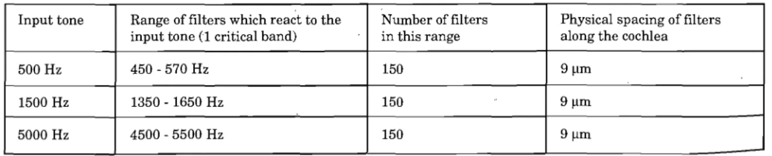
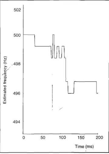
Figure 5 shows a typical estimate of the input frequency as a function of time of a 500 Hz tone of 200 ms duration. This is the frequency estimate after combination ofthe spike rate estimates of each spike train. Only a small fragment ofthe frequency axis is shown. The variance in estimation of the frequency of the tone over the 200 ms period can be seen clearly. Fortunately the input tone is coded bya mul-tiplicity of nerve fibres, arid the variance of the collective estimation of the tone frequency is far smaller than what TABLE 1. Ranges of critical bands around the input tones used in the model.
Input tone Range of filters which rea~t to the Number of filters Physical spacing of fil ters input tone (1 critical band) in this range along the cochlea
500 Hz 450 - 570 Hz 150 9J.lm
1500 Hz 1350 - 1650 Hz 150 9J.lm
5000 Hz 4500 - 5500 Hz 150 9J.lm
ce
d
b
y
Sa
bi
ne
t G
at
ew
ay
u
nd
er
li
ce
nc
e
gr
an
te
d
by
th
e
Pu
bl
is
he
r (
d
at
ed
2
01
88
Input tone
Frequency: f
Duration: T
ENCODER
---1---...
---N cochlear filters spread over one critical
band
Average rate generator Compressive nonlinearity
(spike rate saturation)
AI 1,.2 A) .. ···· .... ··Ai ... AN
Poisson-distributed spike train generator
(spike train i has Poisson intensity Ai)
- -
--
-
-
- - - - -
-
-
-
-
--
-
-
-
--DECO DER
...
---
- -
--
- - - -
-
-
--
- - -
--
- -
--Optimal estimator forPoisson intensity
of each spike train i of N spike trains
A'" I 1,./ A" ) · ... ·Ai' ... ·AN•
Population code decoder Optimal combini3.tion of
N estimated intensities
r~
Frequency jnd determination Calculate standard deviation
of f' over interval T
---~---4/
FIG URE 3. Schematic diagram of the neural encod-ing and decodencod-ing operations implemented in the model. The encoder encodes stimulus parameters (in this case, frequency) in the spike train pattern. The cochlear filters are used to calculate activities of a neural population ofN nerve fibres (e.g., 150 fi-bres) (centred approximately at the input tone fre-quency) in response to the input tone. The amount of activation of each cochlear filter is then used to calculate the appropriate average spike rate for each fibre, using parameters for low spontaneous rate fibres and taking spike rate saturation into account. The N spike trains now carry the neural code for the input frequency. The spike rate (Poisson process intensity) is estimated separately for each spike train. These estimations are then combined to provide an estimate for the input frequency. The frequency jnd is determined by equating it to the standard deviation in estimated frequency over the duration of the stimulus.
would have been expected from figure 4 for one nerve fibre alone.
Relative frequency discrimination jnds (jnd£lf) for hu-mans as measured by Sek & Moore (1995) and Moore (1973) (solid lines) are compared to the predictions from the model (markers) in figure 6. Clearly, although the task of the cen-tral observer seems very difficult (figure 4), the population code is quite effective in representing information about the frequency of a single tone. As was observed by Siebert (1970), we see here as well that, given enough channels in the population code, the ideal central observer does better than human observers in psychoacoustic frequency dis-crimination experiments. This is true when one or two low SR nerve fibres per hair cell were used and where it was assumed that the other nerve fibres do not contribute to frequency discrimination. When there is less than one low SR nerve fibre per hair cell, the central observer does not have enough information and fares worse than the human observer data of Moore (1973).
DISCUSSION
CHARACTERISTICS OF THE MODEL
The central observer in the model presented here is a single black box which models all the signal processing tasks of the central auditory system from the input of the audi-tory nerve signals right through to the final decision that the listener has to make in a typical two-alternative forced-choice psychoacoustical experiment. This model has a number of strengths, but also several shortcomings ..
The trends in the predicted frequency discrimination just noticeable differences are correct. As frequency rises, the relative jndfs also rise. For a model with 150 nerve fibres representing the tone in a population code, the model
pre-11111
I1111111
Ii II
CIl
u;
Q)
160
..>::
0..
!!!- 140
Q)
'§ 120
Q)
..>:: 100
0.. CIl
Q) 80
Cl
~ 60
Q)
>
ell 40 "C
2
20 ell
E
:.:::; 0 CIl
Ul 0 50 100 150 200
Time in milliseconds
FIGURE 4.A typical nerve fibre spike train as simu-lated is shown in (a). The frequency of the tone was 1500 Hz and. the characteristic frequency of the nerve was 1503 Hz. The average rate
t..
was 125 spikes/second. The output,t..
*
of one channel of the estimator is shown in (b). The tone was presented for 200 ms.The South African Journal of Communication Disorders, Vol. 46, 1999
ro
du
ce
d
b
y
Sa
bi
ne
t G
at
ew
ay
u
nd
er
li
ce
nc
e
gr
an
te
d
by
th
e
Pu
bl
is
he
r (
d
at
ed
2
01
A Model of Frequency Coding in the Central Auditory Nervous System dicts values for frequency discrimination jnds close to the
data of ,Moore (1973) at lower frequencies. Furthermore, when human nerve fibre density is taken into account (Spoendlin & Schrott, 1989), around 200 low SR nerve fi-bres are expected in a critical band centred at 500 Hz, 300 fibres at 1500 Hz and 150 fibres at 500 Hz. A curve plotted through the relevant data points in figure 6 (the square at 500 Hz, the circle at 1500 Hz and the square at 5000 Hz) has a bowl shape similar to human frequency jnd£lf data.
It has to be taken into account that the choice of various model parameters influences the ability of the population code to present tonal information accurately. We completely ignored the role of the outer hair cells and also the role that the cochlear nucleus plays in sharpening tuning curtes (Kim, Parham, Sirianni & Chang, 1991). Also, we assumed that high SR fibres do not contribute to the rate-place code.
If they did, the predicted frequency discrimination jnds would decrease.
Furthermore, the role of phase-locking in coding the iden-tity of a single tone was ignored in the present model. But phase-locking is ubiquitous in the peripheral auditory sys-tem and probably plays an important role in the coding of frequency. It was not the purpose of this article to prove the opposite, but rather to indicate how the rate-place code
502
500
N
:r:
-498 >, ( ) / c/
/Q) ::::J
a-Q)
-=
"0
2 ro 496 E
~
UJ
/
494
o
50 100 150 200Time (ms)
FIGURE 5. Estimated frequency as a function oftime for a 500 Hz pure tone input of 200 ms duration. Only a small fragment of the frequency axis is shown to show the variance in estimation of the frequency of the tone clearly. There is a slight bias in the . stimation as well, as the average of the estimated frequency is 498.3 Hz. The standard deviation is 1.4 Hz.
may be interpreted. If the central observer uses phase-lock-ing information as well, listeners should in theory be able to perform far better on frequency discrimination tasks than what has been observed in psychoacoustical experiments. This was also observed by Siebert (1970).
HAIR CELL LOSS
Apart from indicating that the assumption of more nerve fibres contributing to the rate-place code leads to better frequency resolution, figure 6 can also be interpreted as showing the effect of hair cell loss. With a smaller number of available hair cells, the model leads us to expect that frequency discrimination jnds will rise.
CONCLUSIONS
Siebert (1970) predicted the best achievable frequency jnd by other methods, but did not indicate which signal processing the auditory system is required to do to achieve this discrimination threshold. The model presented in this paper proposes a mechanism for the signal processing re-quired for frequency discrimination.
The model clearly shows (as was also remarked by Siebert, 1970), that the human observer does not make full use of all the information relevant to frequency which is available in the auditory nerve spike trains. The reasons for this are not clear. One possibility is that there are other sources of noise not taken into account in this model. It is concluded from the model that the rate-place code alone is adequate to account for frequency discrimination behav-iour in humans.
jndf/f
0.008
0.004 A
0.002
•
0.001
•
0.0005
•
500 1500 5000
Frequency (Hz)
FIGURE 6. Just noticeable difference in frequency (jndf) is normalized by frequency (jndf/f) and plot-ted as a function of frequency. The solid lines are human frequency jndf/f data as measured by Sek & Moore (1995) (curve A) and Moore (1973) (curve b). The squares are thejndflfvalues predicted by the model when a population of 150 nerve fibres is used. Circles are for 300 fibres, triangles for 75 fibres and diamonds for 30 fibres. The datapoints for 75 fibres and 30 fibres coincide at 500 Hz. In all cases the population of nerve
fibres was spread over a range of one critical band around the tone.
ce
d
b
y
Sa
bi
ne
t G
at
ew
ay
u
nd
er
li
ce
nc
e
gr
an
te
d
by
th
e
Pu
bl
is
he
r (
d
at
ed
2
01
90
REFERENCES
Baldi, P. & Heiligenberg, W. (1988). How sensory maps could en-hance resolution through ordered arrangements of broadly tuned receivers. Biological Cybernetics, 59, 313-318. Bialek, W., Rieke, F., de Ruyter van Steveninck, RR & Warland,
D. (1991). Reading a neural code. Science, 252, 1854-1857. Delgutte, B. (1995). Physiological models for basic auditory
per-cepts. In H.L. Hawkins, T.A. McMullan, A.N. Popper & RR Fay (Eds.),Auditory Computation. New-York: Springer-Verlag.
D~lgutte, B. (1997). Auditory neural processing of speech. In w.J.
Hardcastle & J. Laver (Eds.), The handbook of phonetic
sci-ences. Oxford: Blackwell Publishers.
Green, D.M. & Swets, J·.A., (1966). Signal Detection Theory and
Psychophysics. New York: John Wiley and Sons Inc.
Johnson, D.H. (1980). The relationship between spike rate and synchrony in responses of auditory-nerve fibers to single tones.
Journal of the Acoustical Society of America, 68, 4, 1115-1122. Johnson, D.H. & Swami, A. (1983). The transmission of signals by auditory-nerve fiber discharge patterns. Journal of the
Acoustical Society of America, 74, 2, 493-501.
Johnson, D.H. (1996). Point process models of single-neuron dis-charges. Journal of Computational Neuroscience, 3, 275-299. Keidel,W.D., Kallert, S. & Korth, M. (1983). The Physiological
Basis of Hearing. New York: Thieme-Stratton Inc.
Kiang, N.Y-S. (1965). Discharge patterns of single fibers in the
cat's auditory nerve. Cambridge: M.LT. Press.
Kim, D.O. & Molnar, C.E. (1979). A population study of cochlear nerve fibers: comparison of spatial distributions of average-rate and phase-locking measures of responses to single tones.
Journal of Neurophysiology, 42, 1, 16-30.
Kim, D.O. (1984). Functional roles of the inner- and outer-hair-cell subsystems in the cochlea and brains tern. In C. Berlin (Ed.), Hearing Science. San Diego: College-Hill Press. Kim, D.O., Chang, S.O. & Sirianni,J.G. (1990). A population study
of auditory-nerve fibers in unanaesthetized decerebrate cats: response to pure tones. Journal of the Acoustical Society of
America, 87, 4, 1648-1655.
Kim, D.O., Parham, K, Sirianni, J.G. & Chang, S.O. (1991). Spa-tial response profiles ofposteroventral cochlear nucleus neu-rons and auditory-nerve fibers in unanaesthetized decerebrate cats: response to pure tones. Journal of the Acoustical Society
of America , 89, 6, 2804-2817.
Kim, D.O.& Parham, K (1991). Auditory nerve spatial encoding
of high-frequency pure tones: population response profiles derived from d' measure associated with nearby places along the cochlea. Hearing Research, 52, 167-180.
Langner, G. (1992). Periodicity coding in the auditory system.
Hearing Research, 60,115-142.
Moore, B.C.J. (1973). Frequency difference limens for short-du-ration tones. Journal of the Acoustical Society of America, 53, 610-619.
Moore, B.C.J. & Sek, A. (1996). Detection of frequency modula-tion at low modulamodula-tion rates: evidence for a mechanism based on phase locking. Journal of the Acoustical Society of America, 100, 2320-2331.
Moore, B.C.J. (1997). Aspects of auditory processing related to speech perception. In w.J. Hardcastle & J. Laver (Eds.), The
handbook of phonetic sciences. Oxford: Blackwell Publishers. Pouget, A., Zhang, K, Deneve, S. & Latham, P.E. (1998).
Statis-tically efficient estimation using population coding. Neural
Computation, 10,373-401.
Ruggero, M.A. (1992). Physiology and coding of sound in the au-ditory nerve. In A.N. Popper & R Fay (Eds.), The
Mamma-lianAuditory Pathway; Neurophysiology. New York: Springer-Verlag.
Sek, A. & Moore, B.C.J. (1995). Frequency discrimination as a function frequency, measured in several ways. Journal of the
Acoustical Society of America, 97, 4, 2479- 2486.
Shadlen, M.N. & Newsome, W.T. (1994). Noise, neural codes and cortical organization. Current Opinion in Neurobiology, 4, 569-579.
Shofner, w.P. & Sachs, M.B. (1986). Representation of a low-fre-quency tone in the discharge rate of populations of auditory nerve fibers. Hearing Research, 21, 91-95.
Siebert, W.M. (1970). Frequency discrimination in the auditory system: place or periodicity mechanisms? Proceedings of the
IEEE, 58, 5, 723-730.
Smith, RL. (1988). Encoding of sound intensity by auditory neu-rons. In G.M. Edelman, W.E. Gall & W.M. Cowan (Eds.),
Au-ditory Function. Neurobiological Bases of Hearing. San Di-ego: College-Hill Press.
Snippe, H.P. & Koenderink, J.J. (1992). Discrimination thresh-olds for channel-coded systems. Biological Cybernetics, 66, 543-551.
Spoendlin, H. & Schrott, A. (1989). Analysis of the human audi-tory nerve. Hearing Research, 43, 25-38.
Zwicker, E. & Fastl, H. (1990). Psychoacoustics. Facts and
Mod-els. Berlin: Springer-Verlag.
The South African Journal of Communication Disorders, Vol. 46, 1999