Open Journal Systems

(1)

ORIGINAL ARTICLE

An Empirical Test of the Theory of Efficient Markets of Stock Prices

Keshab Bhattarai and Vasi Margariti

University of Hull, Business School, England, UK

Abstract: A structure of the statistical tests motivated by Cromwell, Labys et al.[23]_{has been used to build linear and}

nonlinear predictability models. Most importantly, the variance ratio test and that of AR-GARCH model is used to test the dual hypotheses of the random walk and efficiencyin stock markets. While in all or nothing condition of market efficiency, the variance ratio tests show weak signs of predictability and in contrast to the AR-GARCH model that shows strong signs of predictability. Testing efficiency over time shows that price-fluctuations between periods of predictability and unpredictability and these are not correlated through indices. This study then contributes to the empirical evidence that the efficient market hypothesis should not be an all or nothing condition but be stated as a time varying condition where prices fluctuate between periods of efficiency and inefficiency. It is found that market microstructure can cause problems for certain measuring frequencies and a sufficiently risk averse investor may be happy to pay a premium to avoid any unforecastable asset price volatilities as in Leroy[11]_{and Lucas}[12]_{. Three random walk models also do not}

prevent questioning the validity of predictability of stock prices.

Keywords: predictability and volatility of stock prices; efficient market hypothesis

JEL category: G12, G17

Received: January 18, 2018; Accepted: January 29, 2018; Published Online: September 14, 2018

Citation: Bhattarai K, Margariti V. An Empirical Test of the Theory of Efficient Markets of Stock Prices. Finan Mar, 2018; 3(2); http://dx.doi.org/10.18686/fm.v3i2.1077

1. Introduction

The efficient market hypothesis defines a market in which prices always “fully reflect” available information by Fama[1]_{. An investor can choose among the vast number of shares representing a portion of an underlying firm under the}

assumption that security prices at any time “fully reflect” all available information. This study will only consider one form of market efficiency, namely that of weak-form efficiency where the information set which an efficient market is considered to fully reflect includes only historical prices.

The intentional consequence of weak-form efficiency is that share prices are postulated to be unpredictable from past prices and the process of price formation is random. A direct contrast backed by innumerable evidence by the literature is that historic prices do indeed have predictive power which directly challenges the validity of the efficient market hypothesis. The scope of this study will thus consist of firstly testing whether the weak-form of the efficient market hypothesis holds–or in other words test whether historic share prices do indeed have predictive power. Secondly and most importantly I extend the test for the efficient market hypothesis by examining the predictability of prices over time. If it is deemed statistically appropriate that historic share prices have predictive power whether over time or as an all or nothing condition–or that there is time varying efficiency, the efficient market hypothesis will be rejected.

This is an open-access article distributed under the terms of the Creative Commons Attribution Unported License

(http://creativecommons.org/licenses/by-nc/4.0/), which permits unrestricted use, distribution, and reproduction in any medium, provided the original work is properly cite

(2)

2. Theoretical Foundations of Efficient Market Hypothesis

In the history of thought, an early anticipation of efficient markets comes from the Ph.D. thesis in mathematics submitted by Louis Bachelier in 1900 where he proposes that prices evolve through time following a “random walk”.

Translated in English and published by Cootner, 1964 with the opening paragraph “past, present and even discounted future events are reflected in market price, but often show no apparent relation to price changes”. This is exactly what Fama many years later meant by an informally efficient market. He continues to write “if

the market, in effect, does not predict its fluctuations, it does assess them as being more or less likely, and this likelihood can be evaluated mathematically”. This became known as a random walk. Bachelier considered the fluctuations of bond prices on the Paris Bourse and concluded that prices, pounded by unpredictable fragments of news formed it in such a way that makes it impossible to foretell prices.

While the importance of the work of Bachelier is undisputable and ahead of its time, it was not recognised until many decades later. It is a well-known fact that in the 19th_{century and later, the field of mathematics underwent an}

astonishing increase in the breadth and complexity of mathematical concepts marking fundamental changes to the field. The type of work that Bachelier submitted proved to be a heuristic study lacking rigor in mathematics as well as economics, an unfavourable mix seemingly pointing out why the work went unnoticed for so long. As Cootner[2]_{notes, “compared}

to the standards of rigor at the time, the work of Bachelier was heuristic and scorn for the heuristics led to an underestimation by contemporaries of the significance of the contribution”.

The merit of Bachelier’s work is that his study marked the beginning of the theory of stochastic processes. It anticipated the Chapman-Kolmogorov-Smoluchowski equation for continuous stochastic processes, the derivation of the Einstein-Wiener Brownian motion process and the recognition that this process is a solution of the partial differential equation for heat diffusion and many more analytical results rediscovered by the field some decades later.

2.1 The Random Walk Hypothesis

Bachelier was not the only person to contribute to the studies on the difficulty of predicting capital markets. Cowles[3]

concluded that there is no strong evidence of the ability of predicting capital markets. Working[4] _{came to a similar}

conclusion–that stock returns behave like numbers from a lottery. Kendall[5] _{to his surprise while studying 22 UK stocks}

observed near zero correlation of price changes. Kendall notes “Such serial correlation as is present in these series is so weak as to dispose at once of any possibility of being able to use them for prediction. It may be, of course, that series of individual share prices would behave differently – the point remains open for inquiry. But the aggregates are very slightly correlated and some of them are virtually wandering”. Kendall labels his experiment as a “failure”, reflecting that the results did not sit easily alongside the beliefs of the practitioner and more generally economists of that time and along with Bachelier’s work (arguably for other reasons), which were largely overlooked until early 1960’s.*

Precisely in the early 1960’s, economist Paul Samuelson began to circulate the earlier work of Bachelier concerning the random nature of asset prices among colleagues marking a turning point in the field. The field was able to answer, in theory, how the risk of an investment should affect its expected return leading to the development of the Capital Asset Pricing model by Sharpe et al., 1964. Cootner, 1964 publishes “the random character of stock market prices” in his collection of papers regarding the randomness of price increments. In January 1965 Fama publishes his PhD thesis arguing the random nature of stock prices with concluding remarks “it seems safe to say that this paper has presented strong and voluminous evidence in favour of the random walk hypothesis” followed by the publication of Samuelson’s “Proof that properly anticipated prices fluctuate randomly” in the spring of that year.

Samuelson[6] _{subsequently develops a general stochastic model of prices in which future prices are completely}

(3)

that will result in an expected profit. The quoted price faced by the investor will already contain all that can be known about the future and in that sense, has discounted future contingencies as much as possible.

2.2 Market Efficiency

Before the late 60’s, the price formation process was supposed to be random along with some evidence in support of it. Samuelson’s work marking a turning point in the literature paved the way for Fama[7]_{who incorporated the closely}

related model of random walk into the efficient market hypothesis–a consequence of a specific information subset (weak-form). Along with the weak, semi-strong and strong form suggested to Fama by Harry Roberts, 1967 and a rocky history of efficient markets originating from isolated work (such as Bachelier, Cowles and more) lead him to publish ground-breaking work relating to efficient markets which subsequently earned him the Nobel prize in economics in 2013. The way Fama defined an efficient market is:

“In general terms, the ideal is a market in which prices provide accurate signals for resource allocation: that is, a market in which firms can make production-investment decisions, and investors can choose among the securities that represent ownership of firms’ activities under the assumption that security prices at any time “fully reflect” all available information. A market in which prices always “fully reflect” available information is called efficient”

*_{The only exception before the 1960’s of finding evidence of non-randomness in asset prices is Cowles & Jones, 1937 where they find significant}

evidence of serial correlation in averaged time series indices of stock prices.

Hence the literature of efficient markets of the early 70’s proposed that changes in asset prices are unforecastable if they fully incorporate the expectations and information’s of all market participants then the expected rate of return of a tradeable asset follows a martingale. Evidence was found in support of this. Fama, 1970 wrote “We shall conclude that, with but a few exceptions, the efficient-markets model stands up well,”.

Oscillations in financial markets correspond to oscillations in an investors wealth indicating that there is a strong incentive to disprove the efficient market hypothesis and be able to say that there are patterns in historic prices to be found which will correspond with profitable trades. It brings about interesting studies which show the cases where markets can actually be inefficient. An interesting work on the reason markets can never be efficient using the all or nothing condition comes from Grossman[8]_{and Grossman and Stiglitz}[9]_{on the valid hypothesis that a perfectly informationally efficient}

market is an impossibility since if this is the case then there is no return to compensate for obtaining information. This might shed a light on possible inefficiencies in the market to provide enough return to compensate the obtaining of information. The reason this might possibly happen is of course unclear but one thing is for certain, a trader can never know whether he is trading on information he has or he thinks that he has and is trading on this information. In reality it may turn out that he is not trading on this set of information that he has and indeed this information set is already reflected in prices and in fact he is trading on “noise”.

Black[10]_{in his rather enjoyable paper writes how noise is contrasted with information and how some people correctly}

trade on information expecting to make profits and others trade on noise as if it were information and that “noise trading is essential to the existence of liquid markets”.

Black paints the picture of noise making markets possible but inefficient. Possible because there will be little trading without noise and inefficient because noise creates opportunities to trade with positive profits. Since for a trade to be executed, there needs to be a buyer and a seller, if noise does not exist, “A person with information or insights about individual firms will want to trade, but will realize that only another person with information or insights will take the other side of the trade. From the point of view of someone who knows what both the traders know, one side or the other must be making a mistake. If the one who is making a mistake declines to trade, there will be no trading on information”. Noise then provides liquidity to financial markets, noise trading–that is trading on noise as if it were information. The

(4)

prices. The price of a stock reflects both the information that information traders trade on and the noise that noise traders trade on”

2.3 Recent literature on Efficient Markets

Despite substantial amount of research done after the mid 80’s leading up to research in recent periods it is still surprising to find why the efficient market hypothesis still stands to be accepted or refuted with no clear consensus among financial economists. There is no clear consensus even when the hypothesis is easy to state and has the advantage of exhibiting the most extensive empirical evidence in share prices.

Extensive research points out that the literature of efficient markets is well-established but says little about the problematic nature of the efficient market hypothesis, that of being a joint hypothesis with little hope of ever actually rejecting it. The joint hypothesis problem stems from the fact that testing for efficiency involves assuming an equilibrium model which defines the price formation process. In this study, we use three different versions of the random walk model. If tests result in the rejection of this model, it could mean that the market studied really is efficient or that the price formation process does not follow a random walk.

Before going forward, it is important to note a serious limitation to the random walk model. Samuelson[6]_{derives the}

martingale property for futures (carrying over to equity assets) incorporated into the efficient market hypothesis but it does not account for risk in any way. It mentions nothing about the requirement of the trade-off between risk and expected return. A sufficiently risk averse investor may be happy to pay a premium just to avoid owning an unforecastable security. This was demonstrated by Leroy[11]_{considering models of portfolio selection. With similar conclusions Lucas}[12]_provides

atheoretical examination of the stochastic behaviour of equilibrium prices in a one-good pure exchange economy. The findings of both show that that the efficient market hypothesis will hold, that is prices fully reflect all available information even if the martingale model fails and returns are not completely random.

An added complication to the efficient market hypothesis is time varying efficiency which this study proves through empirical evidence. What encapsulates time varying efficiency is the adaptive markets hypothesis proposed by Lo[13]*

where he suggests that traditional models of financial economics can co-exist alongside behavioral models in an intellectually consistent manner. Lo, 2005[14] _writes:

"Many of the examples that behaviourists cite as violations of rationality that are inconsistent with market efficiency, “loss aversion”, “overconfidence”, “overreaction” and other behavioral biases – are, in fact, consistent with an evolutionary model of individuals adapting to a changing environment via simple heuristics”.

*_{For recent findings regarding AMH see – Urquhart, McGroarty}[19]_{; Lim, Luo, Kim}[16]_{; Urquhart, Hudson}[20]_{; Ghazani&Araghi}[21]_{and more}

interestingly Hull, M. &McGroarty[18]_{; and Alvarez -Ramirez, Rodriguez, Espinosa-Paredes}[22]_.

As interpreted by Urquhart et al.[15]_{, market participants adapt to the ever-changing environment by relying on}

heuristics to make their investment choices hence efficiency varies over time.

Studies that test efficiency of markets over time include Lim et al.[16]_{where it is reported that market efficiency}

varies over time in a cyclical fashion as deemed by rolling sample approach of a Portmanteau bicorrelation test. Todea et al.[17]_{using the same approach of a rolling window subsample report that returns are not constant over some period of}

time but are actually sporadic as deemed by a moving average model. McGroarty, 2014[18]_{show convincing evidence of}

the adaptive markets hypothesis using the Hurst-Mandelbrot-Wallis rescaled range test as a measure of market efficiency over emerging markets. Urquhart[19]_{apply three versions of variance ratio tests and a filtered GARCH model and conclude}

that price predictability varies over time with periods of significant predictability on returns but also periods of no predictability.

(5)

3. Theory of Efficient Markets

3.1 The efficient market hypothesis

The statement that an efficient market “fully reflects” available information is presented by Fama notationally as:

𝐸(𝑝̃𝑗,𝑡+1|Φ𝑡) = [1 + 𝐸(𝑟̃𝑗,𝑡+1|Φ𝑡)]𝑝𝑗𝑡 (1)

where𝑝𝑗𝑡 denotes the price of asset j at time t, 𝑝̃𝑗,𝑡+1 is the random variable of the price of asset j at time 𝑡 + 1, the percentage return 𝑟̃𝑗,𝑡+1as defined in section IV: a, the information set symbolΦ𝑡represents a general symbol for the set of information assumed to be fully reflected in the price at time 𝑡.

Equation (1) favours generality, that is, as pointed out by Fama, the expecteddifference between the actual return (next period) and hypothesized equilibrium expected return𝐸(𝑟̃𝑗,𝑡+1|Φ𝑡) should be zero. 𝐸(𝑟̃𝑗,𝑡+1|Φ𝑡) is determined by the chosen expected return theory–the joint hypothesis that whatever equilibrium returns model is applied, the information set Φ𝑡 (defined below) is “fully” utilised in determining equilibrium expected returns. The model used in this study will be that of the random walk model which will be carefully introduced in the next subsection.

The information set can take the following forms:

o The weak-form efficiency: In the weak-form efficiency, the information set includes only historical prices.

o The semi-strong-form efficiency: the information set includes historical prices and also all publicly available information, that is the adjustment of security prices to publicly available information or information generating event such as stock splits, announcements of financial reports by firms, new security issues etc.

o The strong-form efficiency: the information set contains all of the information in the weak and semi-strong form and additionally including private information and insider trading.

3.2 The random walk hypothesis

The random walk hypothesis proposes that the price formation process of stock market prices follows a random process–that is, the expectancy of future returns is an independent and identically distributed process–a random walk. The random walk model is popular among social sciences as well as physical sciences where it is favoured for its simplicity and elegance.

The random walk model will be presented in accordance to the seminal work of Lo et al.[23]_{which organise various}

versions of the random walk by considering various kinds of dependence that can exist between an asset’s prices 𝑝𝑡= ln 𝑃𝑡 and 𝑝𝑡+𝑘= ln 𝑃𝑡+𝑘 at two dates 𝑡 and 𝑡 + 𝑘.

3.2.1 Independent and identically distributed increments

The first and the most simplistic version of the random walk model is that the disturbance term is independently drawn from the same distribution with the same mean and variance. Normal and IID disturbance terms in asset prices can be modelled by building the relationship between the natural logarithm of prices follows a random walk with normally distributed increments:

𝑝𝑡= 𝜇 + 𝑝𝑡−1+ 𝜖𝑡 𝑝𝑡− 𝑝𝑡−1= 𝜇 + 𝜖𝑡

(6)

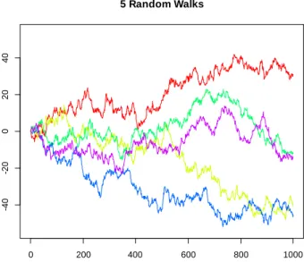
Figure 1. Simulated random walk trajectories of length 1000 with normally distributed increments

This is equivalent to the discrete version of Brownian motion sampled at equal-spaced intervals which can be stimulated by taking cumulative sums of standard normal distributions (withμ=0) which can be simulated using R programming in Figure 1.

The assumed behaviour of the disturbance term is often too strong and not realistic of share prices therefore the model would have the other two variations of the random walk would have to somehow account forthese violations of the first model of the random walk model.

3.2.2 Independent increments

The second version of the random walk hypothesis relaxes the assumption of identically distributed increment allowing heteroskedastic disturbance terms. It still assumes that all increments are independent but they are not drawn from the same distribution, it accounts for each disturbance term being drawn from different distributions. Modifying (2) gives:

𝑟𝑡= 𝜇 + 𝜖𝑡, 𝜖𝑡 ~ 𝐼𝑁𝐼𝐷 (0, 𝜎2) (3)

0 200 400 600 800 1000

-4

0

-2

0

20

40

5 Random Walks

time

va

lu

e

0 1 2 3 4

0

1

2

3

4

5

6

7

Heteroscedastic data

x

y

(7)

which is a broader definition that includes (2). What is important however is that moving from the first model to the second allows for unconditional heteroskedasticity in the disturbance terms – it permits time varying fluctuation if and only if the disturbance terms are independent and not correlated or satisfy the conditional probability density function:

𝑝𝑑𝑓(𝜖𝑡+𝑘|𝜖𝑡) = 𝑝𝑑𝑓(𝜖𝑡+𝑘) (4)

Modelling independent increments which includes the first random walk model given by (2).

3.2.3 Uncorrelated increments

In this third and final form of the random walk hypothesis considered, the assumption of uncorrelated increments still holds but that increments need not be independent and permit processes with dependent but uncorrelated increments. Campbell, Lo et al.[23]_{propose that all possible versions of the random walk model can be captured by the orthogonality}

condition with two arbitrary functions 𝑓(∙) and 𝑔(∙) (and for disjoint t, k):

𝑐𝑜𝑣[𝑓(𝜀𝑡), 𝑔(𝜀𝑡+𝑘)] = 0 (5)

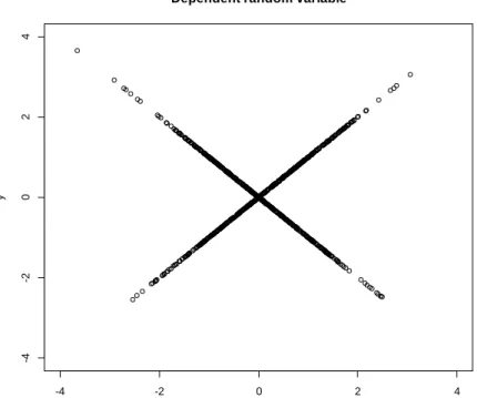
but if functions 𝑓(∙) and 𝑔(∙) were restricted to linear functions, then (5) clearly implies that they are not serially correlated but they are transformed by a linear function making them dependent as illustrated by Figure 3 above. This is the version of the random walk which will be tested in this study using a series of statistical tests given in section IV.

3.3 Wiener process and SDE

Since the purpose of this study is not only to test the efficient market hypothesis but also provide a thorough history of efficient markets, a slight digression will show what was meant in the literature review in section II that the random walk originates from Bachelier by presenting a version of the work completed byBachelier as presented by J.Voit[24]_{. The}

derivation which Bachelier carries out stems from examining the probability density 𝑝(𝑥, 𝑡) of a price change of a certain size𝑥 at some time 𝑡 in the future. Although this work will avoid pointing out his heuristic significances and his mistakes

-4 -2 0 2 4

-4

-2

0

2

4

Dependent random variable

y

(8)

it will show that he still managed to give a strong theory of the randomnature of stock markets related to the Brownian motion, around 5 years prior to Einstein’s famous work.

If 𝑝(𝑥1, 𝑡1)𝑑𝑥1is the probability of a price change of interval [𝑥1, 𝑥1+ 𝑑𝑥1] at time𝑡1 and similarly 𝑝(𝑥2, 𝑡2)𝑑𝑥2 is the probability of a price change of interval [𝑥2, 𝑥2+ 𝑑𝑥2] at time𝑡2, Bachelierthen derives the probability density function of a price change by considering the joint probability of the dual theoretical price change :

𝑝(𝑥1, 𝑡1)𝑝(𝑥2− 𝑥1, 𝑡2)𝑑𝑥1𝑑𝑥2 (6)

Which naturally leads to the probability of a change of 𝑥2 at 𝑡1+ 𝑡2: 𝑝(𝑥2, 𝑡1+ 𝑡2)𝑑𝑥2= [∫ 𝑝(𝑥1, 𝑡1)𝑝(𝑥2− 𝑥1, 𝑡2)𝑑𝑥1

∞ −∞

] 𝑑𝑥2 (7)

This presents the physics equation known as Chapman-Kolmogorov-Smoluchowski equation-something which was noted in the introduction that Bachelier anticipate. Bachelier solves this equation by the Gaussian normal distribution to obtain the result:

𝑝(𝑥, 𝑡) = 1

√2𝜋𝜎(𝑡)exp (− 1 2

𝑥2

𝜎2_(𝑡)) (8)

which is clearly directly related to Brownian motion or the formulation of the random walk, or equivalently the “Einstein-Wiener Stochastic process”.

A theoretical example with homoscedastic and independent Gaussian increments can be presented through stochastic differential equations. Based on Øksendal, 2003[25]_{and lecture notes on Stochastic differential equations Goodman}[26]_a

stochastic differential equation can be considered:

𝑑𝑋𝑡= 𝑎𝑡𝑑𝑡 + 𝑏𝑡𝑑𝑊𝑡 (9)

This differential equation with 𝑑𝑊𝑡 denoting the standard wiener differential presents 𝑑𝑋𝑡 as the sum of a deterministic piece which models the part of 𝑑𝑋𝑡 that is known at time 𝑡 and a random piece which models the part of 𝑑𝑋𝑡 that is not deterministic and not known at time 𝑡 (what Bachelier derived). This kind of set up permits the creation of models of stochastic processes by writing expressions for the above 𝑎𝑡 and 𝑏𝑡getting an equation of the form:

𝑑𝑋𝑡= 𝑎(𝑋𝑡, 𝑡)𝑑𝑡 + 𝑏(𝑋𝑡, 𝑡)𝑑𝑊𝑡 (10)

Where 𝑎𝑡 and 𝑏𝑡 are functions of two variables completely known at time 0. By considering a discrete version of the above, and taking into consideration the assumptions of the Brownian motion mentioned above would yield the result:

𝑋𝑡= 𝑋0+ ∫ 𝑎(𝑠, 𝑋𝑠)𝑑𝑠 + [∫ 𝑏(𝑠, 𝑋𝑠)𝑑𝑊𝑠 𝑡

0

] 𝑡

0

(11)

Where the term on the bracket defines, a random variable called the stochastic Ito Integral of b. This presents 𝑋𝑡 as a stochastic process satisfying the above equation. The definition of the wiener process causes problems when solving for the integral in the square brackets in equation (11) above since the function is not differentiable at any point and has infinite variation over every time interval. This has important theoretical implications for this study since loosely speaking the integrand 𝑏(𝑠, 𝑋𝑠)would need to be adapted using Ito calculus by constraining that the value of this integrand at time t can only depend on information available until time t. The evolution of an asset price is an example of this logic. Such model with 𝑆𝑡 the share price at time 𝑡 replacing 𝑋𝑡, the expected rate of return 𝜇 replaces 𝑎(𝑋𝑡, 𝑡) and the volatility 𝜎

(9)

replacing 𝑏(𝑋𝑡, 𝑡) in the model above can be represented by:

𝑑𝑆𝑡= 𝜇𝑆𝑡𝑑𝑡 + 𝜎𝑆𝑡𝑑𝑊𝑡 (12)

Statistical properties of asset returns talk about how stock prices are believed to be event driven, that is, news affects the price formation process or has impact. A single piece of news can of course affect say two assets but it is intuitively sound to expect that the impact that the news has on prices will differ between stocks, indices etc. but this does not mean that asset returns do not show similarities in movements. By the study of asset prices by the literature, it is widely accepted that there are empirical facts exhibited by asset prices.

1. absence of autocorrelation 2. heavy tails

3. gain/loss asymmetry 4. aggregational gausianity 5. intermittency

6. volatility clustering 7. conditional heavy tails

8. slow decay of autocorrelation in absolute returns 9. leverage effect

10. volume /volatility correlation 11. asymmetry in time scales

4. Statistical Framework

4.1 Prices

Based on the transformations presented by Campbell, Lo et al.[23]_{the raw data of share prices will be normalisedfor}

the benefit of better statistical properties (stationarity, normality etc.), that is the data will be measured in a comparable metric of continuously compounded return between dates 𝑡 − 1 and 𝑡 where it is assumed that the share price does not pay dividend:

𝑟𝑡(𝑘) = ln (∏ ( 𝑃𝑡−𝑗+1

𝑃𝑡−𝑗 ) 𝑘

𝑗=1

)

= ∑ log (𝑃𝑡−𝑗+1 𝑃𝑡−𝑗

) 𝑘

𝑗=1

= ∑ 𝑟𝑡−𝑗+1 𝑘

𝑗=1 ₍₁₃₎

Equation (15) represents a flow variable of horizon k and in this study a horizon bigger than 1 will not be used to equation (15) will collapse to:

𝑟𝑡= log ( 𝑃𝑡 𝑃𝑡−1

(10)

= log(𝑃𝑡) − log (𝑃𝑡−1)

= 𝑝𝑡− 𝑝𝑡−1 (14)

This is the definition of a one period return that will be used in this study whenever returns are considered–allowing for the assumption of a lognormal distribution.

4.2 Stationarity

Testing for stationarity is perhaps the first thing that ought to be done with time series; that is, the sample statistics should be defined in such a way that they are invariant with respect to time. If a process is found to be nonstationary through the appropriate tests then the data needs to be transformed to convert the process to stationary.

4.2.1 Augmented dickey-fuller test

This study will adopt the augmented Dickey-Fuller test which examines the sample data with the objective of answering whether the process has a unit root and whether diferencing will remove the unit root.

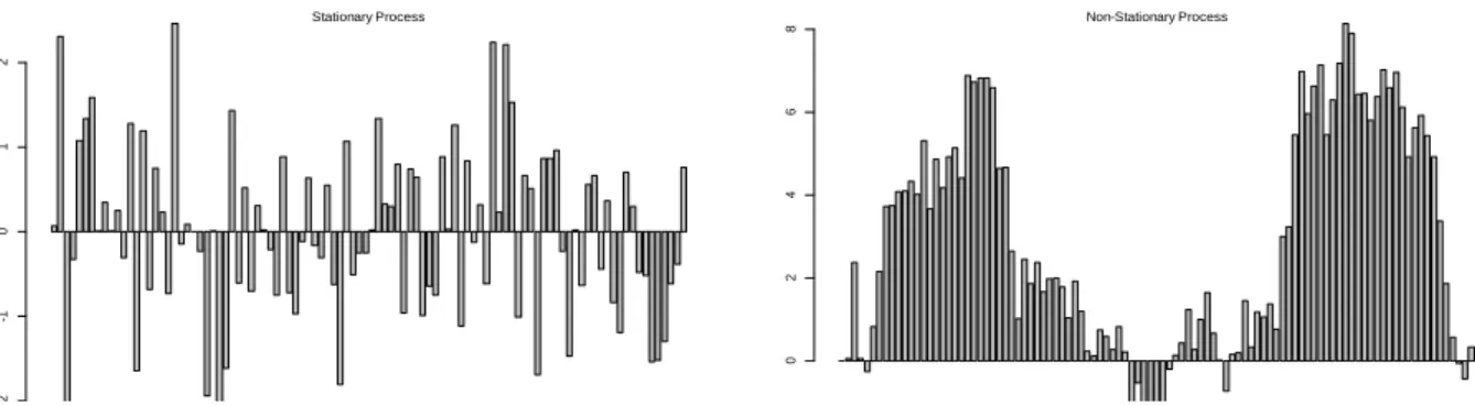
Using a simple simulation of some random numbers which are plotted in the left hand side of Figure 4, and a

-2

-1

0

1

2

Stationary Process

0

2

4

6

8 Non-Stationary Process

-3 -2 -1 0 1 2 3

-3

-2

-1

0

1

2

Normal Q-Q Plot

Theoretical Quantiles

S

a

m

p

le

Q

u

a

n

ti

le

s

Histogram of Normal Distribution

x

F

re

q

u

e

n

cy

-3 -2 -1 0 1 2 3

0

20

40

60

80

100

Figure 5. Simulation of a stationary process (left) and its undoing (right) Figure 4. Simulated QQ plot against normal distribution·

(11)

transformation of this data caried out by applying discrete integration (inverse of differencing) which are plotted on the right hand side of Figure 4. Both data sets, the random and the transformed will then be subject to the Dickey-Fuller test which results in accepting its alternative hypothesis of stationarity at the 1% significance level for the random numbers and accepting the null hypothesis of non-stationarity for the transformed data where the difference is undone confirming what is clear visually in Figure 4.

4.3 Normallity

4.3.1 QQplot

A useful graphical way to test for normality of a time series is by comparing a time series to the normal distribution using the quantile-quantile plots. This is achieved by plotting normal theoretical quantiles of the normal distribution in the horizontal axis for comparison with sample quantiles of some given data plotted in the horizontal axis. In general, if the line fitted to the plot is steeper a 45-degree line through the origin, it implies that the distribution is not equal and that the sample distribution in the vertical axis is more dispersed than that of the horizontal axis. What the individual points of the sample data should follow is a 45-degree line from the origin and since probabilistically this will only occur at very rare occurrences, stimulating this graphic technique by using the normal distribution for both axis will give basis of comparison to what the data should look like if it does follow a normal distribution plotted in Figure 5 above.

4.4 Testing for Independence

An important feature of the random walk which is shared by all three variations of the models given in section III-Bis that all autocorrelations of the increments are zero including the third and weakest form of the random walk where dependency is permitted.

4.4.1 Ljung-Box

A simple test statistic following autocorrelation is the 𝒬-statistic as presented by Box et al. 1970 and later expanded by Ljung et al.[27]_:

𝒬𝑚= 𝑇(𝑇 + 2) ∑ 𝜌(𝑘) 𝑇 − 𝑘 𝑚

𝑘=1

(15)

which is asymptotically distributed according to the Chi-Squared distribution. This test is used to pick up any departures from zero autocorrelations in either direction at all lags. The null hypothesis suggests that the time series is independent thus when the null hypothesis is satisfied (15) is asymptotically Chi-Squared distributed with k degrees of freedom.

4.4.2 BDS

Through statistical testing of a time series, the variation in the data could be deemed as random and suggest that it follows the normal distribution but although a time series could provide enough statistically significant evidence that it does follow the normal distribution and it is random, it can also exhibit chaotic behaviour where a time series is deemed normal but it is still possible to find deterministic components. The Brock-Dechert-Scheinkman has been proven to have high power against such behaviour and univariate models which this study will consider. Cromwell et al.[28]_{present the}

BDS statisticas a test of independence by embedding the time series in m-space:

𝑟𝑡𝑚= [𝑟1, 𝑔 𝑡𝑟𝑡−𝑚+1], 𝑡 = 1, 2, … , 𝑇 − 𝑚 + 1 (16)

The motivation behind this is that the dependence of a time series can be examined defining a measure of distances between the subjective m-space and some chosen distance 𝜀. This metric is defined as:

𝕀[𝑟𝑡𝑚, 𝑥𝑠𝑚; 𝑠] = {

1, 𝑖𝑓 ‖𝑟𝑡𝑚− 𝑥𝑠𝑚‖ ≤ 𝜀 0, 𝑜𝑡ℎ𝑒𝑟𝑤𝑖𝑠𝑒

(12)

(17)

The purpose of doing so is to study the correlation integral of the time series where under these conditions it is given by:

𝐶(𝜀, 𝑚, 𝑇) = ∑ 𝕀[𝑟𝑡

𝑚_{, 𝑥𝑠}𝑚_{; 𝑠]} 𝑡≠𝑠

[𝑇𝑚(𝑇𝑚− 1)]

(18)

Since the correlation integral (18) estimates the probability of the distance between the above pairs of points being less than or equal to 𝜀, the test proposes that if the observations are indeed independent, this probability will just be the product of the individual probabilities assigned to each pair. This is of course unknown and the test statistic that is used to estimate it isthe asymptotically standard normally distributed test statistic:

𝑊(𝜀, 𝑚, 𝑇) = 𝐶(𝜀, 𝑚, 𝑇) − 𝐶(𝜀, 1, 𝑇) 𝑚

4𝑇(𝐾(𝜀)𝑚_{+ 2[𝜗])} 𝑎

→ 𝒩(0, 1)

(19) where 𝜗 is given by:

𝜗 = ∑ 𝐾(𝜀)𝑚−𝑖_𝐶(𝜀)2𝑖_{+ (𝑚 − 1)}2_𝐶(𝜀)2𝑚_{− 𝑚}2_{𝐾(𝜀)𝐶(𝜀)}2𝑚−2 𝑚−1

1

(20)

and 𝐾 is the probability of a three-tuple of points being within 𝜀 distance of each element. When testing, a common approach is to set the distance element 𝜀 a multiple of the standard deviation of the time series being tested and the m-space from 2–4. A large emphasis will be put on the p values of this test in section V where prices will be tested for predictability. The approach will be that the distance element 𝜀 will be set to the standard deviation of the time series and the mean of the output statistic by the 2 m space dimensions selected.

4.5 Linear autocorrelation

4.5.1 Serial Correlation

Perhaps a simpler computation which tests the random walk model, perhaps one that is less difficult to implement illustrates the case where the relationship between a time series and its lagged values can be represented by a linear equation. Such an example can be the autoregressive model AR(k):

𝑟𝑡= 𝜇 + 𝑟𝑡−1+ 𝑢𝑡 (21)

where the disturbance term 𝑢𝑡 is generated by the process:

𝑢𝑡= ∑ 𝜌𝑖𝑢𝑡−𝑖 𝑘

𝑖=1

+ 𝜖𝑡, 𝜖𝑡 ~ 𝐼𝐼𝐷 𝑁(0, 𝜎2)

(22)

Given a time series, measuring the relationship of a random variable at time 𝑡 and its value 𝑘 periods earlier can also be calculated by the autocorrelation equation:

𝜌(𝑘) =𝐶𝑜𝑣[𝑟𝑡, 𝑟𝑡+𝑘] 𝑉𝑎𝑟[𝑟𝑡]

(23)

(13)

of the same series at different dates. Under the random walk hypothesis, the increments of the random walk are all uncorrelated at all lags thus a test of the random walk hypothesis could be built by testing whether financial data shows signs of serial correlation, and if they do, the price data will be deemed predicttable, a violation of the efficient market hypothesis.

4.5.2 Variance ratio tests

Lo et al.[29]_{take advantage of the important property of the random walk that the variance of its increments must be}

a linear function of the time interval. This can be proved by using calculations from Dougherty[30] _{where he proposes that}

the distributional changes through time can be shown mathematically by supposing the following relationship:

𝑟𝑡= 𝑟𝑡−1+ 𝜖𝑡 (24)

and by lagging and substituting t times,

𝑟𝑡= 𝑟0+ 𝜖1+ 𝑦 𝑙𝑎𝑔𝜖𝑡−1+ 𝜖𝑡 (25)

And given that the initial value 𝑟0 is zero and with our assumptions of the disturbance term, the estimated value of 𝑟𝑡 is also zero. The variation through time can now be decomposed as:

𝑣𝑎𝑟(𝑟𝑡) = 𝑣𝑎𝑟(𝜖1+ 𝜖2+ ⋯ + 𝜀𝑡)

= 𝑣𝑎𝑟(𝜖1) + 𝑣𝑎𝑟(𝜖2) + ⋯ + 𝑣𝑎𝑟(𝜀𝑡) = 𝜎𝜖2_{+ 𝜎𝜖}2_{+ ⋯ + 𝜎𝜖}2

= 𝑡𝜎𝜖2 ₍₂₆₎

This demonstrates that the random walk model has the property that the variance of its increments is linear or in other words, it says that the variance of 𝑝𝑡− 𝑝𝑡−2 should be twice the variance of 𝑝𝑡− 𝑝𝑡−1 if the null hypothesis is indeed correct.

The linearity of the variance of the random model can be illustrated visually through Figure 6 in the previous page where it plots 1500 independent realisations of the random walk with zero mean and a unit variance. From this simulation,

(14)

Using the fact that the random walk exhibits linear variance through time, Lo et al.[29] _{construct a test statistics of the}

random walk hypothesis using variance ratios by considering a 𝑘 period return 𝑟(𝑘) as given by (13) at the beginning of this section and compare the differences in variance by the relationship:

𝑉𝑅(𝑞) =𝑣𝑎𝑟[𝑟𝑡(𝑞)] 𝑞 𝑣𝑎𝑟[𝑟𝑡]

=𝑣𝑎𝑟[𝑟𝑡+ 𝑟𝑡−𝑞+1] 𝑞 𝑣𝑎𝑟[𝑟𝑡]

= 1 + 2 ∑ (1 −𝑘 𝑞) 𝜌(𝑘) 𝑞−1

𝑘=1 (27)

where 𝜌(𝑘) is the kth order autocorrelation coefficient of 𝑟𝑡. Under the random walk model, the variance ratio test statistic should be equal to 1, that is𝑉𝑅(𝑞) = 1 𝑞 and 𝑘 > 1.

The data will consist of 𝑛𝑞 + 1 observations (i.e. 𝑟0, 𝑟1, 𝑏𝑠𝑒𝑟𝑟𝑛𝑞 of 𝑟𝑡) and the unknown population parameters are 𝜇 and 𝜎2_{to which Lo, Mackinlay}[29]_{present the maximum likelihood estimators defined by:}

𝜇̂ = 1

𝑛𝑞(𝑝𝑛𝑞− 𝑝0)

(28)

𝜎̂𝑎2(𝑞) = 1

𝑛𝑞 − 1∑(𝑝𝑘− 𝑝𝑘−1− 𝜇̂) 2 𝑛𝑞

𝑘=1 (29)

𝜎̂𝑏2(𝑞) =

𝑛𝑞

𝑞(𝑛𝑞 − 𝑞)(𝑛𝑞 − 𝑞 + 1)∑(𝑝𝑘− 𝑝𝑘−𝑞− 𝑞𝜇̂) 2 𝑛𝑞

𝑘=𝑞 (30)

𝑉𝑅̂ (𝑞) =𝜎̂𝑏 2_(𝑞) 𝜎̂𝑎2

(31)

As elegant as this is–a sampling distribution of (31) will have to be considered under the third and weakest model of the random walk (uncorrelated increments). This allows of course a much wider range of time series–specifically the concencus of the literature is that volatilities change over time so a sampling distribution of (31) would need to permit dependence on the type and degree of heteroskedasticity present so as long as returns are not correlated (31) should still approach one. Lo et al.[29] _{then propose a heteroskedasticity consistent estimator:}

𝜉̂(𝑞) = ∑ [2(𝑞 − 𝑗)

𝑞 ]

2_{𝑛𝑞 ∑} _(𝑝

𝑘− 𝑝𝑘−1− 𝜇̂)2(𝑝𝑘−𝑗− 𝑝𝑘−𝑗−1− 𝜇̂) 2 𝑛𝑞

𝑘=𝑗+1

[∑𝑛𝑞𝑘=1(𝑝𝑘− 𝑝𝑘−1− 𝜇̂)2] 2 𝑞−1

𝑗=1

(32)

And given this, the standardised test statistic is given by:

𝑍(𝑞) =√𝑛𝑞(𝑉𝑅̂ (𝑞) − 1) √𝜉̂

𝑎

→ 𝒩(0, 1) (33)

The null hypothesis then assumes that returns possess uncorrelated increments while allowing for general forms of heteroskedasticity. If the null hypothesis is rejected, it means that the test has found significant evidence of price predictability, a violation of the random walk model and of the efficient market hypothesis (the joint hypothesis).

(15)

4.6 Non-Linear Dependence (in variance)

4.6.1 Generalized autoregressive conditional heteroskedasticity

The variance ratio test statistic above permits deterministic changes in variance due to seasonal factors and dependency of the conditional variance on past information. It is of interest to study the conditional variance on past information further. This relates to models of changing volatility. A model hoping to explain oscillations in stock prices would be very far from reality if it assumed that volatility of the series would be constant through time thus, to capture these patterns in volatility an ARCH model is considered. Originally proposed by Engle (1982) and presented by Campbell et al.[23]_as:

𝜎2_{= 𝜔 + 𝛼(𝐿)𝜀𝑡}2 ₍₃₄₎

The authors present the conditional variance as a distributed lag of past square innovations𝜀𝑡2 where 𝜔 is the variance intercept, 𝛼 the parameter of the model and lastly 𝛼(𝐿) is a polynomial in the lag operator.

A more powerful approach to testing conditional variance is through a GARCH (p, q) model which will be tested later using R software through acolossal package in size In R programming language called “rugarch” by Alexios Ghalanos[31]_{. A thorough and enlightening presentation of the mathematics behind the code is also provided by the author}

which presents the dynamics of conditional mean allowed by the univariate GARCH specification as: Φ(𝐿)(1 − 𝐿)𝑑_(𝑦

𝑡− 𝜇𝑡) = Θ(𝐿)𝜀𝑡 (35)

Equation (43) presents the fractional AR model on demeaned data and MA model on the residuals with mean defined by:

μt= 𝜇 + ∑ 𝛿𝑖𝑥𝑖,𝑡 𝑚−𝑛

𝑖=1

+ ∑ 𝛿𝑖𝑥𝑖,𝑡𝜎𝑡+ 𝜉𝜎𝑡2 𝑚

𝑖=𝑚−𝑛+1 ₍₃₆₎

The above is the filtration process for where its residuals 𝜀𝑡2_{will be of use in the GARCH (p, q) model first introduced} by Bollerslev[32]_{. Conditional variance as presented by Ghalanos, 2015 is the long-form equation:}

𝜎2_{= [ 𝜔 + ∑ 𝜁𝑗𝑣𝑗𝑡} 𝑚

𝑗=1

] + ∑ 𝛼𝑗𝜀𝑡−𝑗2 𝑞

𝑗=1

+ ∑ 𝛽𝑗𝜎𝑡−𝑗2 𝑝

𝑗=1 (37)

with 𝜔 denoting the intercept. The term ∑𝑚𝑗=1𝜁𝑗𝑣𝑗𝑡 inside the square brackets allows the possibility of passing external regressors, something I will not do, in fact equations (35) will be defined as an AR(p) process where the optimal p will be chosen up to 10 lags (thus removing all linear dependence) and equation (37) will be transformed into a GARCH (1, 1) without external regressors yielding: *

𝑟𝑡= 𝛾0+ ∑ 𝛾𝑖𝑟𝑡−1 𝑝

𝑡=1

+ 𝜀𝑡, 𝜀𝑡~𝑁(0, 𝜎𝑡2)

𝜎𝑡2= 𝜔 + 𝛼1𝜀𝑡−12 + 𝛽1𝜎𝑡−12 (38)

What will be subject to test for nonlinear dependence will then be the residuals of the model presented in (38) as determined by the BDS statistic in section IV-C. If this test finds nonlinear dependence in conditional volatility, it is a violation of the efficient market hypothesis.

(16)

The sample data consists of daily, weekly, and monthly prices of three of the most important indices in the world– namely FTSE 100, S&P500 and NIKKEI225. The time series are obtained from Bloomberg which cover a snapshot of prices of about 27 years, from 1 January 1990 to early 2017. Monthly time plots of the data obtained is provided in Figure 7 which allows for a visual interpretation of the changes in price experienced by the three indices. For comparison purposes the FTSE 100 and S&P 500 are significantly higher now than they were in 1990. Both indexes have gone through substantial growth periods in the timeline observed. The exception of growth given the upper and lower bound of the sample time interval is Nikkei 225 which is considerably lower now compared to what it was in the 90’s. The two indices that have experienced growth in the snapshot provided, namely FTSE 100 and S&P 500 show that they tend to evolve very like each other over time. Incorporated in the timeline is severe economic downturn. The timeline starting in 1990 perfectly captures the “lost decade–the past 10 years’ of the Japanese economy where the asset price bubble collapsed hardly picking up in the 20’s. Both the UK and American economy experienced recessions in the early 90’s and early

20’s through the collapse of the speculative dot-com bubble signified by the large drops in Figure 7. Most severe of them all is the great recession which all three economies felt with prices of the NIKKEI taking significantly longer to recover compared to the FTSE and S&P.

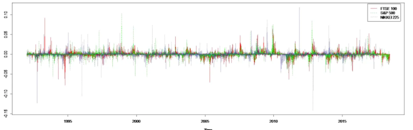
Taking the first difference of the logarithm of prices transforms the data presented in Figure 7 to one period returns which are ploted in Figure 8 below.it is observed that the series oscillates around zero, precisely as is expected. Observing how returns change as time evolves, the duration and amplitude of each positive and negative sequence is of course thought to be random but there seems to be a rather weak tendency for positive returns to be followed by positive returns and negative returns to be followed by negative returnshence visually the reurns data of the three indices shows signs of weak autocorrelation.It is not easy to analyse data visually but something could be said about the volatility of the three indices by comparing the magnitude of the returns. NIKKEI 225 seems to be more volatile than the FTSE 100 and S&P 500 because the bars in the returns data in Figure 8 seems to be more erratic and extend higher than those of S&P 500 and that of FTSE 100, something

Figure 7.Monthly time plots of FTSE 100, NIKKEI 225 and S&P 500 through a 27-year period

2000

3000

4000

5000

6000

7000

ft

se

.p

ri

ce

10000

20000

30000

n

ikke

i.

p

ri

ce

500

1000

1500

2000

1990 1995 2000 2005 2010 2015

sp

.p

ri

ce

ts(index.monthly, start = c(1990, 1), frequency = 12)

S&P 500 FTSE 100

(17)

that is confirmed with the standard deviation results in Table 1 below. Table 1 shows that the mean of the three indices for daily, weekly and monthly frequencies is practically 0.

Index OBS Mean SD Skewness Kurtosis JB ARCH(10)

Daily Returns

FTSE100 6865 0.000160 0.011136 -0.126790 8.927857 10068*** 1504.5***

S&P500 6852 0.000275 0.011225 -0.245229 11.737153 21863*** 1690.9***

NIKKEI225 6657 -0.000105 0.015417 -0.130005 8.237658 7626.9*** 1130.3***

Weekly Returns

FTSE100 1417 0.000779 0.023252 -0.788169 12.733412 5736.2*** 164.88***

S&P500 1418 0.001349 0.022776 -0.740082 9.802852 2861.7*** 210.56***

NIKKEI225 1413 -0.000503 0.030874 -0.673395 8.437368 1846.1*** 72.808***

Monthly Returns

FTSE100 324 -0.003337 0.040788 0.526317 3.594557 19.731*** 24.405***

S&P500 324 -0.005973 0.041758 0.782599 4.777047 75.705*** 30.171***

NIKKEI225 324 0.002335 0.063174 0.474469 3.905917 23.164*** 19.446**

Table 1. Descriptive statistics of returns for FTSE 100, NIKKEI 225 and S&P 500. *, **, *** indicates significance at 10%, 5%, 1% respectively.

All the indices also exhibit negative skewness which implies a longer left tail. The distribution of all the return time series are leptokurtic since excess kurtosis is observed. The test for normality through the Jarque-Berra shows strong signs

Time

Figure 7. Monthly time plots of FTSE 100, NIKKEI 225 and S&P 500 through a 27-year period

-0

.2

-0

.1

0

.0

0

.1

0

.2

FTSE 100 Monthly return

-0

.2

-0

.1

0

.0

0

.1

0

.2

NIKKEI 225 Monthly return

-0

.2

-0

.1

0

.0

0

.1

0

.2

S&P 500 Monthly Returns

(18)

Finally using the standard deviation of the three series as a basic measure of volatility, indicate that NIKKEI 225 has the highest level of volatility and FTSE 100 the least level of volatility. A stronger method of extracting more information from the data set is to implement a rolling standard deviation of returns over a subsample which moves forward through time in Figure 9.*_{This is what was implemented by the literature to study time varying volatility before specifying more}

complicated univariate models such as models of conditional volatility (see Officer, 1973[33]_{; Garman,}_{et al.}_{, 1980}[34]_;

Parkinson, 1980[35]_{; Merton, 1980}[36]_{). Merton, 1980 observed that this method accurately measures volatility at some}

point in time if an assets price follows the geometric Brownian motion equation (12) included in section III-C. From Figure 9, it is easy to see that the volatility of the FTSE 100 seems to follow that of S&P while NIKKEI 225 almost always never intersects the other two lines indicating earlier suspicions that the volatility of NIKKEI 225 is much higher than that of the FTSE 100 and that of the S&P 500.

logarithmic differencing and plotting the transformed standard deviation of all three indices which is illustrated in Figure Time

Time

Figure 9. Rolling plot of monthly standard deviation through time for FTSE 100, NIKKEI 225 and S&P 500 Bringing the attention to the dashed line represenging the volatility of NIKKEI 225, the 10 year period called the “lost decade” mentioned earlier is clearly associated with very high volatility in comparison to the other two indices which only show spikes around periods of economic downturn whith the biggest volatility measured around the great depresion of late 2008. Clearly Figure 9 is non-statinoary. By switching to daily frequency and removing the unit root through

(19)

Daily Prices

WeeklyPrices

MonthlyPrices

Daily Returns

WeeklyReturns

MonthlyReturns

10 will capture the motivation for conditional variance models presented later. This plot shows that volatility varies widely across the indices and through time but this variation is done so within a range which itself changes slowly over time.

5.2 Stationarity

Typically share prices have a unit root, that is the mean and volatility is not independent through time but this can be accounted for by using the definition of returns as the logarithmic difference of lagged raw prices as defined in section IV-A. The price process is a difference-stationary process, that is taking the difference of the lagged logarithmic raw price data will convert the non-stationary process that has a unit root to a stationary process which does not have a unit root. This is confirmed in Table 2 in the next page where raw price data and returns are subject to the augmented Dickey-Fuller test. The first three columns of Table 2 shows that the null hypothesis of the presence of a unit root is accepted for nearly all data sets consisting of raw prices with one exception of NIKKEI 225 daily.

Index OBS ADF statistic Index OBS ADF statistic

FTSE100 6865 -2.2541 FTSE100 6865 -19.829***

S&P500 6852 -1.2742 S&P500 6852 -19.49***

NIKKEI225 6657 -3.6774** NIKKEI225 6657 -18.184***

FTSE100 1417 -2.0406 FTSE100 1417 -12.545***

S&P500 1418 -1.1523 S&P500 1418 -11.199***

NIKKEI225 1413 -2.915 NIKKEI225 1413 -11.194***

FTSE100 324 -2.3097 FTSE100 324 -6.5882***

S&P500 324 -1.6862 S&P500 324 -6.4179***

NIKKEI225 324 -3.0963 NIKKEI225 324 -6.9912***

Table 2. Augmented Dickey-Fuller test applied to raw prices and returns. *, **, *** indicates significance at 10%, 5%, 1% respectively.

The differenced data however in the last three columns of Table two shows that the Augmented Dickey-Fuller test rejects the possibility of a unit root at the 1% significance level – the transformed data is stationary.

5.3 Normality

A statistical tool with emphasis on simplicity is the QQ plotproviding the means of examining the returns process departure from normality. By plotting returns as a transformed and standard normal variable in the vertical axis as a linear function of the standard normal distribution in the horizontal axis to provide means of comparison. This plot should exhibit a straight line of 45-degrees from the origin if 𝑟𝑡 is normally distributed. As mentioned in section IV-C, a straight

(20)

if the deviation is significant, then it points out that the returns process is not similar to the normal distribution therefore it is not normally distributed. This probability plot is presented in Figure 11 below which provides a plot for each index at its three frequencies of measurement chosen for this study.

It is easy to notice that most of the points fall in the middle of the plot but start to curve off as the points start to

Figure 11. QQ plot for daily, weekly and monthly returns of FTSE 100, NIKKEI 225 and S&P Monthly

reach the two most extreme values of returns on both sides, that is the points form an elongated “s” implying that the tails of returns are actually longer than that of the normal distribution. This does not prove that returns are not random, it merely shows that the distribution of returns has fat tails. A very important feature of Figure 11 which will be expanded on later is that it has found evidence that a change in frequency, that of daily to weekly and weekly to monthly makes the returns data appear more normal.

5.4 Independence

The starting point for testing the random walk model is to test returns forindependence. Table 3 below presents the test statistic of returns of all three indices of two tests considered, the Ljung-Box test and the BDS test.

Index OBS 𝑄1 𝑄2 𝑄3 𝑊2 𝑊3 𝑊4

Daily Returns

-4 -2 0 2 4

-0 .1 0 0 .0 0 0 .1 0

FTSE 100 daily

Theoretical Quantiles S a m p le Q u a n til e s

-4 -2 0 2 4

-0 .1 0 0 .0 0 0 .1 0

NIKKEI 225 daily

-4 -2 0 2 4

-0 .1 0 0 .0 0 0 .1 0

S&P 500 daily

-3 -2 -1 0 1 2 3

-0 .2 -0 .1 0 .0 0 .1

FTSE 100 weekly

-3 -2 -1 0 1 2 3

-0 .2 0 .0 0 .1

NIKKEI 225 weekly

-3 -2 -1 0 1 2 3

-0 .2 0 -0 .0 5 0 .0 5

S&P 500 weekly

-3 -2 -1 0 1 2 3

-0 .1 0 0 .0 0 0 .1 0

FTSE 100 monthly

-3 -2 -1 0 1 2 3

-0 .2 0 .0 0 .2

NIKKEI 225 monthly

-3 -2 -1 0 1 2 3

-0 .1 5 -0 .0 5 0 .0 5

S&P 500 monthly

(21)

FTSE100 6865 1.0314 14.125*** 32.215*** 17.0946*** 23.4161*** 28.7452***

S&P500 6852 20.256*** 31.772*** 31.834*** 15.0497 *** 22.6668*** 28.0077***

NIKKEI225 6657 5.2805** 13.008*** 13.095*** 11.2117*** 16.1150*** 19.6809***

Weekly Returns

FTSE100 1417 7.0205*** 9.8207*** 21.001*** 5.8770*** 8.7768*** 10.4373***

S&P500 1418 9.0158*** 14.111*** 18.12*** 9.7412*** 11.8071*** 14.1955***

NIKKEI225 1413 0.97723 6.6926** 7.6598* 6.5281*** 7.1768*** 7.7931***

Monthly Returns

FTSE100 324 0.13084 0.99667 1.1865 4.0448*** 6.1001*** 7.3554***

S&P500 324 0.92438 1.0047 2.2568 4.0350*** 5.6732*** 7.1109***

NIKKEI225 324 0.80252 0.81071 1.3617 1.2519 1.9043* 2.7079***

Table 3. Ljung – Box and BDS test statistic applied to returns. *, **, *** indicates significance at 10%, 5%, 1% respectively.

In the first panel of Table 3, the test statistics show strong signs of autocorrelation as deemed by both statistics at the 1% significance level. When moving to the second panel, that of weekly returns, the BDS statistic still shows significant level of autocorrelation detected while the Ljung-Box weakens from daily to weekly. For monthly data, the BDS statistic still remains highly significant for all three indices but the Ljung-Box statistic weakens entirely reporting no significant findings of autocorrelation. The null hypothesis of the Ljung-Box statistic is actually independence, what is required for the first and second models of random walk while the third random walk permits dependence with the requirement that increments are uncorrelated. This study thus finds evidence through the Ljung-Box statistic that there is some degree of predictability in returns for daily frequency but this gets weaker as the frequency measurement decreases. The more powerful test, that of BDS remains significant regardless of frequency because it could be evidence for time varying conditional variance.

5.4.1 Linear autocorrelation

Table 4 presents the computed value of the AR(k) process with order varying from 1 to 16. The test shows that most of the serial correlation detected is through the first panel of the data, that of daily frequency. Although it does show signs of autocorrelation, this is indeed very weak and transitioning from daily frequency to weekly frequency weakens this even more to findings suggesting that there is even less evidence of serial correlation in the data. For monthly frequency in the third panel of Table 4, there is not a single statistically significant test statistic. This pattern was noted when examining probability plots in the previous section and also in the Ljung-Box test statistic in Table 3. This could be due to the effects of market microstructure which will be discussed in a future section but also it is worth noting that the sample size does indeed change when the frequency is changes as depicted by the dotted line

Index OBS 𝜌̂1 𝜌̂2 𝜌̂3 𝜌̂4 𝜌̂10 𝜌̂16

Daily Returns

FTSE100 6865 -0.012 -0.044* -0.051* 0.036* -0.004 0.011

(22)

NIKKEI225 6657 -0.028* -0.034* -0.004 -0.015 0.023 -0.014

Weekly Returns

FTSE100 1417 -0.070* 0.044 -0.089* -0.026 -0.030*** 0.013

S&P500 1418 -0.080* 0.060* -0.053* -0.025 0.002 0.014

NIKKEI225 1413 -0.026* 0.064 -0.026 0.000 -0.041 0.000

Monthly Returns

FTSE100 324 0.020 -0.051 -0.024 0.097 -0.048 0.011

S&P500 324 0.053 -0.016 0.062 0.047 -0.001 0.021

NIKKEI225 324 0.050 -0.005 0.041 0.017 0.017 -0.011

Table 4. Autocorrelation in daily, weekly and monthly index returns

Figure 12 below. Overall through the AR process, evidence of weak and negative autocorrelation is found.

0 5 10 15 20