Sharif University of Technology
Scientia IranicaSpecial Issue on: Socio-Cognitive Engineering http://scientiairanica.sharif.edu
An ecient hardware implementation for a motor
imagery brain computer interface system
A. Malekmohammadi, H. Mohammadzade
, A. Chamanzar, M. Shabany, and
B. Ghojogh
Department of Electrical Engineering, Sharif University of Technology, Tehran, Iran. Received 9 August 2017; received in revised form 30 March 2018; accepted 4 August 2018
KEYWORDS Brain Computer Interface (BCI); Electroencephalograph (EEG);
Motor imagery; Field Programmable Gate Arrays (FPGA); Separable Common Spatio Spectral Pattern (SCSSP); Support Vector Machine (SVM); Linear Discriminant Analysis (LDA).
Abstract.Brain Computer Interface (BCI) systems, which are based on motor imagery, enable humans to command articial peripherals by merely thinking about the task. There is a tremendous interest in implementing BCIs on portable platforms, such as Field Programmable Gate Arrays (FPGAs) due to their low-cost, low-power and portability characteristics. This article presents the design and implementation of a Brain Computer Interface (BCI) system based on motor imagery on a Virtex-6 FPGA. In order to design an accurate algorithm, the proposed method avails statistical learning methods such as Mutual Information (MI), Linear Discriminant Analysis (LDA), and Support Vector Machine (SVM). It also uses Separable Common Spatio Spectral Pattern (SCSSP) method in order to extract features. Simulation results prove achieved performances of 73.54% for BCI competition III-dataset V, 67.2% for BCI competition IV-dataset 2a with all four classes, 80.55% for BCI competition IV-dataset 2a with the rst two classes, and 81.9% for captured signals. Moreover, the nal reported hardware resources determine its eciency as a result of using retiming and folding techniques from the VLSI architecture' perspective. The complete proposed BCI system achieves not only excellent recognition accuracy, but also remarkable implementation eciency in terms of portability, power, time, and cost. © 2019 Sharif University of Technology. All rights reserved.
1. Introduction
Nowadays, humans attempt to communicate with the outside world in a better and more convenient way. Although, at rst glance, physical transactions seem essential for this goal, science is trying to make this relationship independent of physical actions.
Brain Computer Interface (BCI) is a system, enabling humans to control objects by merely mak-*. Corresponding author.
E-mail addresses: [email protected] (A. Malekmohammadi); [email protected] (H. Mohammadzade); chamanzar [email protected] (A. Chamanzar);
[email protected] (M. Shabany);
ghojogh [email protected] (B. Ghojogh) doi: 10.24200/sci.2018.4978.1022
ing decisions and thinking about them, i.e., without any sort of intervention of physical movement. In other words, a BCI system is an interface between the brain and computer to translate, process, and classify the electroencephalograph (EEG) signals [1]. After classication, this system sends commands to external devices, such as a wheelchair, to control it (Figure 1). A motor imagery system controls articial devices by solely thinking about them. Movements of an articial hand by thinking about its movement is one of the various examples of the applications of such systems, which is a predominant strategy for motor rehabilitation in stroke patients. Note that BCI systems are meant to be wearable, yet not sensible, in future applications; hence, it will be convenient and transparent to others. Moreover, BCI technology as a classication system is well established and has
Figure 1. Functional model of a BCI system. The BCI system can command devices in order to help people with disabilities.
various applications, for instance, for patients with paraplegic devices. Therefore, any eort to improve its performance and/or ecient implementation is needed and valuable.
Although there exist several other controlling approaches, especially for patient or elderly care, motor imagery BCI system has some advantages over them. For instance, eye tracking [2] is not applicable in case the patients have visual or eye muscle problems, such as Amyotrophic Lateral Sclerosis (ALS) and Locked-In Syndrome (LIS), and, therefore, cannot control their eye muscles to move their eye in a certain direction [3-5]. Other problems of eye tracking can be found in dim light conditions or where the patient needs to notice his/her surrounding which would be dangerous for them to move their eye in other directions (e.g., when a patient in a wheelchair is passing on the street). Moreover, people with glasses can use BCI system much more conveniently than those with eye tracker can. Apart from their dierences, both eye tracking and motor imagery BCI require a wearable device; eye tracker requires a pair of glasses to hold a camera to track eye, and BCI system requires a hat with electrodes. Moreover, note that despite the advantages of BCI system over eye tracking, eye tracker has the advantage of higher accuracy in comparison to motor imagery BCI.
In particular, in motor imagery BCI system, when a subject imagines moving, a typical desynchronization of upper alpha and beta rhythms is observed in the sen-sorimotor cortex [6], followed by a re-synchronization. This pattern of activation can be easily detected by EEG and used to feed a BCI system for dierent purposes. In fact, imagination movement tasks evoke EEG signal changes in a way that these changes can be detected in temporal and spatial traces of EEG rhythmic components, at specic electrodes (chan-nels) located on subjects' scalps. Therefore, we can use electrophysiological properties of motor imagery as temporal, spatial and frequency characteristics to detect the mental task. This paper focuses on BCI systems that are based on translating EEG signals recorded through motor imagery.
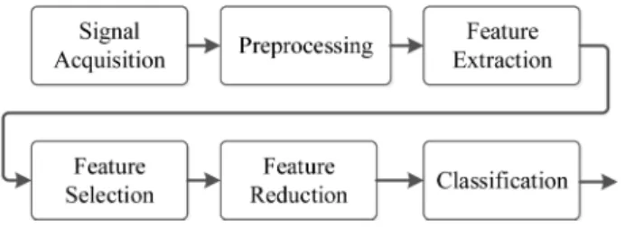
A BCI system consists of units of signal acquisi-tion, preprocessing, feature extracacquisi-tion, feature selec-tion/reduction and classication. Signal acquisition unit records the brain activates such as EEG signals, while the pre-processing unit increases the
signal-to-noise ratio of the signals. On the other side, feature extraction unit prepares features that are meaningful to the classication stage and omits outlier and artifact features. Then, the feature selection/reduction unit reduces the number of features and/or acquisition channels to decrease the dimension of feature vectors. Finally, classication unit classies the features into logical control signals.
Solving a BCI problem includes two phases, i.e., the train and test phases. In the train phase, the parameters of the system are adjusted through learning from previously recorded samples. In the test phase, the new data are recorded and its class is estimated using the parameters adjusted in the train stage. Un-fortunately, such algorithms require high-speed com-puters to process the steps of BCI, limiting their use and portability. Therefore, an ecient algorithm to meet these specications is needed to be designed. In order to overcome this shortcoming, using hardware platforms such as Field Programmable Gate Arrays (FPGAs), which are more portable, less expensive, and power ecient, seems reasonable. Moreover, there are other reasons to use FPGA for implementing a BCI system. First, the parallelism of FPGAs can be used for high computational throughput, especially at low clock rates. Second, FPGAs are more exible and more power-ecient than processors are. Third, FPGAs are more suitable for real-time embedded solutions [7].
This paper proposes an ecient high-accurate algorithm for classication of EEG signals for a BCI system. Moreover, the paper presents an ecient hardware implementation of the proposed BCI on a FPGA platform. The proposed algorithm is based on statistical learning methods, and the hardware implementation considers the optimization of power, area, and frequency to meet the targeted specications of end applications. The achieved results show that the proposed BCI can classify EEG signals from BCI competition IV (4 classes), BCI competition III (3 classes), and our in-house signals (2 classes) with accuracy rates of 67.2%, 73.54%, and 81.9%, respec-tively. The hardware implementation results validate the successful implementation of the proposed method on hardware at the clock frequency of 560 kHz.
The remainder of this paper is organized as follows: In Section 2, the current literature is pre-sented and discussed; in Section 3, all datasets used in this paper are presented; Section 4 describes the proposed methodology for the BCI system. Section 5 shows the simulation results of software, and Section 6 discusses signal processing concerns for hardware im-plementation. The detailed hardware implementation is presented in Section 7. Section 8 discusses some trade-os between accuracy and hardware resources. In Section 9, the obtained hardware experimental results are reported. Finally, Section 10 concludes the paper.
2. Previous work
There is a rich literature addressing the research in BCI systems, where each paper may consider a specic part of the system. The related literature can be divided into two main categories: algorithms and hardware implementation. In the following, state-of-the-art work from each category is briey described.
2.1. Previous work on algorithms
There exists a large amount of literature on BCI algorithms and methods. Two main sub-categories are methods of feature extraction and those of classica-tion:
1. Feature Extraction: Adaptive Auto-Regressive (AAR) is one of the suitable algorithms to extract features from EEG signals [8-10]. A classical approach to estimating time-varying AR-parameter is the segmentation-based approach. In this case, the data are divided into short segments and the AR parameters are estimated from each segment. The shorter the segment length, the higher the time resolution; however, it has the disadvantage of an increasing error in AR estimations. The AAR model appropriately describes the random behavior of EEG signals and provides parameters with a high time resolution. Moreover, by using AAR model, it is not necessary to use frequency band [11]. In [12], an AR model is utilized because of achieving better estimations of short time series compared to Fast Fourier Transform (FFT). AAR can also be used to remove artifacts, such as eye blinking and muscle movements, from EEG data, based on blind source separation [13].
However, the AR model cannot capture the transient features in EEG data, and the time-frequency information is not easily seen in the AR parameters [14]. Therefore, several researchers have used wavelet coecients that provide localization of signal components with spectro-temporal charac-teristics [15-19]. The main benet of wavelets is the frequency localization. The advantage of time-frequency localization is that the wavelet analysis changes the time-frequency aspect ratio, providing a good frequency localization at low frequencies for long time windows and good time localization at high frequencies for short time windows [20]. On the other hand, the Power Spectral Density (PSD) is another approach that indicates the dis-tribution of power of a signal between dierent frequencies [21].
Various other algorithms have also been pro-posed that extract features in spectral or spatial domains such as the Common Spatial Patterns (CSP), classifying brain tasks. In fact, CSP, using the variance as a new feature, tries to extract
features that are able to maximize the variance of a particular task and minimize the variance of the other [22]. A signicant drawback of CSP is that it does not consider the spectral characteristics of the EEG signal [23]. To overcome this problem, many researchers have proposed several variants of CSP [24-27]. One of the promising algorithms for the feature extraction, which is an advanced version of CSP, is called Filter Bank Common Spatial Patterns (FBCSP) whose advantage is that it considers the spectral characteristics of the EEG signals [28,29]. Moreover, an advanced version of FBCSP is called Separable Common Spatio Spectral Pattern (SCSSP) [30], which overcomes all shortcomings of FBCSP, i.e., the high compu-tational cost of training, lack of analysis of both spatial and spectral characteristics of signals, and lack of having a metric to rank the discriminatory power of extracted spatio-spectral features. In addi-tion, CSP methods suer from sensitivity to noise and, also, overtting. In order to overcome these problems, dierent methods are proposed in the literature for regularizing CSP, namely Regularized CSP (RCSP). In [31], various RCSP algorithms are reviewed and summarized, as well as the standard CSP. Thereafter, four novel RCSP methods are proposed and evaluated which outperform previous RCSP methods.
2. Classication: Linear classiers, such as Linear Discriminant Analysis (LDA) and Linear Support Vector Machine (SVM), can be applied to distin-guish classes using linear functions [32]. Methods such as [33-36] have used these classiers in BCI systems. LDA is suitable for online BCI systems because of a low computational cost, which per-suades researchers to use it in motor imagery-based BCI systems. However, the main shortcoming of LDA is its linearity that can provide poor results on complicated nonlinear EEG data [37]. LDA can also be used for feature reduction in EEG signals [38], as is used in the proposed method, too. On the other hand, Linear-SVM uses a discriminant hyperplane to classify EEG features. This method is very popular because of good generalization properties [39], simplicity in implementation, and robustness [40]. Nonlinear classication, such as Bayesian and K-Nearest Neighbors (KNN), are used in [41-43]. Nonlinear methods show better classication performance than the linear methods; however, they are more complicated, especially from the implementation point of view. In spite of all these eorts, designing an ecient algorithm for classication in BCI systems, while considering the hardware constraints, is still a major chal-lenge.
2.2. Previous work on hardware
Most of the literature in which a full BCI system is im-plemented are concentrated on the steady-state visual Evoked Potential, which is an EEG signal response to the ickering visual stimulus [44], [45], [46]. However, in [47], a BCI system is implemented based on motor imagery, which includes Finite Impulse Response lter as a preprocessing, CSP as a feature extraction, and Mahalanobis distance as a classication, on Stratix IV FPGA Board with operational frequency of 200 MHz. This paper proposes a more ecient hardware implementation with less hardware resources compared to the design in [47]. A more complete work of [47] is reported in [48]. A novel approach is introduced in [48], dening the tasks and working with devices by a state machine. The user can do the task or switch to other tasks by thinking about right and left hand movements. There exist several other works on BCI systems with a hardware implementation perspective. For ex-ample, Wearable Mobile EEG-based Brain Computer Interface System (WMEBCIS) [49] is proposed for detecting drowsiness. A low-cost FPGA-based BCI multimedia control system is also proposed in [50]. Their proposed framework is used to control multime-dia devices. In their work, they use Steady-State Visual Evoked Potential (SSVEP), which is light-emitting diode stimulation panel (several command symbols). SSVEP is also utilized in [51] to control environmental devices such as television. Controlling hospital bed nursing system in a FPGA-based BCI system is also addressed in [52].
2.3. Best-performing methods on BCI competition datasets
There are reported accuracies on BCI competitions available in BCI competition web site [53]. The best reported method (in [54]) on BCI competition III-dataset V, which has classied all three classes of this dataset, has used LDA to extract features from PSD values of the EEG signals and distance-based discriminator for classication. The best performing method (as reported in [55]) on BCI competition IV-dataset 2a, which has classied all four classes of this dataset, has employed FBCSP and Naive Bayes Parzen Window as feature extraction and classication, respectively. However, the main shortcoming of these methods is that they provide low accuracies and are not suitable for hardware implementation as they have high computational complexity.
However, the methods proposed in [31] and [48], mentioned previously, outperform the best methods reported in [54] and [55], and can be considered as two of the best performing methods on BCI competition IV-dataset 2a. Nonetheless, it should be noticed that these two methods only classify the rst two classes (movements of right and left hands).
3. Description of datasets
There are two available methods for recording the EEG signals, i.e., invasive and non-invasive methods. The former implants the electrodes in the brain through an operation; thus, it can be dangerous and harmful to the brain. However, the latter records the signals by electrodes on the head skin. In order to standardize the placement of the electrodes on the head, the 10-20 standard has been introduced. In this standard, the distance of adjacent electrodes from each other is 10% or 20% of the whole distance between back (inion) and front (nasion) of the skull. This standard has improved over the years and has multiple versions. Figure 2 depicts the locations of almost all sensors in these standards.
Recording brain signals in the non-invasive ap-proach is commonly called Electroencephalograph (EEG) [56]. The EEG method has some advantages and disadvantages. In fact, a lower price, high time resolution, and robustness of movement could be mentioned as its advantages, and low SNR, distilled water requirement and low spatial resolution are its disadvantages.
Capturing EEG signals, in the lab, consists of multiple steps. After the appearance of the xation cross, a cue is performed to warn the experienced per-son to start thinking about a particular task, which is the motor imagery step. The last step is resting, which happens before starting the next experiment. Figure 3 illustrates the steps of the EEG signal capturing.
In this paper, three datasets are used to verify the proposed algorithm, which are detailed in the sequel. 3.1. BCI competition III - dataset V
One of the datasets used to evaluate the proposed algorithm is dataset V of BCI competition III [53]. This dataset was created by IDIAP Research Institute. Recorded signals are brain signals from three dierent persons, each of which is involved in the experiment for four times. All these four experiments were performed in one day with 5-10 minutes break between every session. The sampling rate is 512 Hz and 32 channels have been used to record the signals. There are both raw signals and power spectral densities available in this dataset; however, only raw signals are used in this paper. In this dataset, each person is asked to think about the following three tasks in dierent time slots:
Imagination of repetitive self-paced left-hand move-ments;
Imagination of repetitive self-paced right-hand movements;
Generation of words beginning with the same ran-dom letter.
Figure 2. Locations of sensors in dierent versions of 10-20 standard.
Figure 3. Timing scheme of the signal capturing paradigm. The paradigm includes xation cross and cue followed by motor imagery and rest.
3.2. BCI competition IV - dataset 2a
The second dataset used in this paper is dataset 2a of BCI competition IV [53], consisting of signals from nine people. Signals from each person are captured in two sessions on dierent days. Each session consists of 6 parts and each part includes 48 experiments. In each experiment, every person is asked to do one of the following four motor imagery tasks:
Imagination of left-hand movements; Imagination of right-hand movements; Imagination of both legs movements; Imagination of tongue movements.
The sampling rate is 50 Hz and data are ltered by a band-pass Butterworth lter.
3.3. Captured signals
In order to devise a local platform to evaluate the algorithms, we managed to record EEG signals by an Emotiv® system, including 14 channels with the
sampling rate of 128 Hz. The EEG electrodes have been placed in locations AF3, F7, F3, FC5, T7, P7, O1, O2, P8, T8, FC6, F4, F8, and AF4 based on International 10-20 system (see Figure 2). Eight persons were asked to imagine performing one of the following two tasks in each experiment:
Imagination of left-hand movements; Imagination of right-hand movements.
Four experimental sessions were held in one day, each of them including 30 experiments. All subjects were sitting on a comfortable armchair in front of a computer screen during the recording session. A ses-sion takes eight seconds, including two seconds to show a xation cross on the black screen at the beginning of session, one second for a cue pointing either to the left or right on the display, three seconds for performing the corresponding task in front of the black screen to avoid visual feedback, and two seconds in order to relax their minds (see Figure 3). The rst three experimental sessions are used as training data, and the last one is used as test data. Before starting to record, all subjects were asked to practice with the experimental conditions
Figure 4. The overall block diagram of the proposed method. The proposed method consists of signal acquisition, preprocessing, feature extraction, feature selection, feature reduction, and nally classication.
for ve minutes in order to reduce their stress and increase their concentration by becoming familiar with conditions. Subjects were asked not to move or blink during these three seconds of motor tasks in order to reduce the eects of artifacts such as electromyogram (EMG) and electrooculography (EOG). Signals were ltered by a highpass lter with 0.1 Hz cut-o fre-quency and, then, ltered by a notch lter with the frequency of 50 Hz to remove the power line eect. Moreover, note that, in the captured signals, subject 7 is about 60 years old, and the other subjects are young, around 23. The signicant dierence between the accuracy rates for subject 7 compared to the other subjects might be due to the older age of this subject. 4. Methodology
The method in this paper consists of several compu-tational blocks, utilized in both train and test phases. Figure 4 shows dierent parts of this method. Each part will be discussed in detail in the following. 4.1. Pre-processing
Preprocessing, which tries to remove noises and arti-facts, is crucial to obtaining high classication accuracy in BCI systems. In the proposed method, two tech-niques, i.e., DC-block and Laplacian lter, are used for this purpose.
1. DC-block: Filtering is an important step to remove unnecessary information from raw signals. In this paper, the xed point DC blocker [57] is applied to remove the DC shifts. The DC component in EEG signals varies between dierent recording runs, even for a specic subject. This component does not include any information regarding the motor imagery task and may degrade the accuracy of the algorithm. Based on this fact and for the sake of achieving stability during all recording runs, the DC component should be omitted by means of a DC lter. An eective solution from the hardware implementation point of view is the DC-blocker, which performs the DC ltering by means of minimum hardware resources based on the following equation [57]:
H(z) = 1 z 1
1 z 1; (1)
where = 0:996:
2. Laplacian Filter: One of the most important limitations of EEG signals is their poor spatial resolution. One common technique in order to alleviate this problem is the Surface Laplacian (SL) ltering [58]. It is also used to remove the noises and artifacts whose origin may be outside of the skull [59], which eventually improves the Signal-to-Noise Ratio (SNR). There are four dierent spatial lters, namely standard ear reference, Common Average Reference (CAR), small Laplacian and the large Laplacian. We employed the CAR method as it has been proven that the CAR is suitable for a communication system related to and rhythms, which are the main frequency bands (8-12 Hz and 12-32 Hz, respectively) (some works, such as [60,61], cite the range of rhythm as 18-30 Hz) for motor imagery EEG signals [62]. In fact, in the CAR method, the potential of each channel (electrode) is subtracted by a weighted average of the next-nearest neighbor channels, according to their distance. If the distances are equal, it can be easily formulated as follows:
VCAR
i = ViER n1 n
X
j=1
VER
j ; (2)
where VER
i is the potential between the ith
elec-trode and the reference, and n is the number of electrodes in the montage.
4.2. Feature extraction
Feature extraction is the process of distinguishing pertinent signal characteristic (i.e., features related to the user's intent) from unnecessary contents. The most popular methods in this eld are AAR, wavelet-based, PSD and SCSSP, described in the sequel.
1. AAR: Autoregressive (AR) method is a simple, yet ecient, method for describing probabilistic behavior of a time sequence. In this paper, AAR is used for the adaptive estimation of the AR parameters [9]. The mathematical expression of this method can be written as follows:
yk = k 1
X
i=k p
aiyi+ xk; (3)
where xk is a Gaussian noise with zero mean and
variance 2
x, parameter p is the degree of AR model,
and ai's are AR coecients. Moreover, k is a
positive number, denoting the number of samples and is related to the signal duration as k = t f0,
where f0 is the sampling frequency.
frequency localization in the time window, which is, in particular, appropriate for signals with transient nature such as EEG. The Wavelet coecients are obtained through decomposition of the signal into dierent frequency bands. This decomposition is performed in multiple stages by means of consecu-tive low-pass and high-pass signal ltering. In this paper, this method is applied to nd the coecients of the frequency bands of and rhythms as features of EEG signals.
3. PSD: In this method, the power of the signal be-tween dierent frequencies is considered as features. Herein, the value of PSD is computed in each 2 Hz frequency band within the 8-30 Hz to cover and rhythms [21].
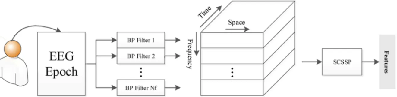
4. SCSSP: Separable Common Spatio Spectral Pat-tern (SCSSP), proposed in [30], improves the Com-mon Special Patterns (CSP) method [22]. This method selects proper features of the signals as illustrated in Figure 5. Let us consider an EEG experiment with Nch channels (electrodes) and Ni
samples. After passing these signals through a set of Nf band-pass lters, Nimatrices with the size of
Nf Nch are obtained. Let X denote a Nf Nch
matrix, and then its spectral (i) and special ( i)
covariance matrices are computed as follows: i= N1
chNi Ni
X
n=1
XXT;
i= N1 fNi
Ni
X
n=1
XTX; (4)
where Ni is the number of training samples X.
Then, by solving the generalized eigenvalue prob-lems in Eq. (5):
1WL= (1+ 2)WLL;
1WR= ( 1+ 2)WRR; (5)
desired eigenvectors (WL and WR) and eigenvalues
(L and R) are calculated.
Following this calculation, components k are
computed as follows: k = i[k]L j[k]R
i[k]L j[k]R + (1 i[k]L )(1 j[k]R ); (6) where i[k]L and j[k]R are components of L and R
eigenvalue matrices, respectively, and k is between 1 and NfNch ks values are then sorted in
descend-ing order, and the rst d is selected in order to determine the corresponding indices i[k] and j[k]. Therefore, the features are obtained as follows:
yk= wTL;i[k]XwR;j[k] for k 2 R;
R =
1; NfNch; 2; (NfNch 1); :::;
d
2; (NfNch d 2 + 1)
; (7)
where wL;i[k] and wR;j[k] are the eigenvectors in
WL and WR corresponding to i[k]L and j[k]R , and
yk can also be found as follows:
yk= (wR;j[k] wL;i[k])TX; (8)
where denotes Kronecker product.
It is suggested to use the normalized log-power features instead, which are calculated as follows:
zk = log
var(yk)
P
k2Rvar(yk)
; (9)
where zk is the kth feature. The feature vector is
then constructed as Z = [z1; zNfNch; :::]T.
Notice that the SCSSP method is a binary-classication algorithm. To generalize it for multi-class purposes, several auxiliary approaches, such as One-Versus-Rest (OVR), can be used.
Finally, the band-pass ltering is performed using Chebyshev type II lters of order 6 and bandwidth of 4 Hz. A total of Nf= 4 lters are used to cover and
Figure 5. Structure of SCSSP algorithm. The EEG signals with Nisamples obtained from Nchchannels pass through Nf
band-pass lters, and a three-dimensional matrix with the size of Nf Nch Ni is obtained. Afterwards, the SCSSP
rhythms. The reasons for using this type of lter are as follows: IIR lters need extremely fewer coecients than FIR lters do; therefore, they require much less hardware resources to implement in comparison to FIR lters. Hence, an IIR lter type is applied. Among IIR lters, Elliptic and Chebyshev type I lters have ripples in their band pass, causing adverse inuence on the nal results. The Chebyshev type II Filter is sharper in the cut-o frequency than Butterworth Filter is. Therefore, better accuracy can be expected from Chebyshev type II lter.
4.3. Normalization
Normalization of features limits their dynamic range and improves the accuracy of the algorithm. It can be performed in both linear and non-linear forms. Assume that mkand kare mean and standard deviation of the
kth dimension of feature vector (Z), respectively: mk =N1
N
X
i=1
Zik; (10)
2
k = N1 1 N
X
i=1
(Zik mk)2; k = 1; 2; :::; l; (11)
where N is the number of training samples. Then, the linear normalization of the train and test Zk is
calculated as follows: ^
Zk =Zk mk
k : (12)
4.4. Feature election
To reduce the number of obtained features eciently, the following two methods can be used:
1. FDR: Fisher Discriminant Ratio (FDR) is a ratio that considers the best features by maximizing the distance between the means of the classes and minimizing the variance within each class. Features that satisfy longer FDR are better ones to be selected.
If i and i denote the mean and standard
deviation of feature Zkin the ith class, respectively,
the FDR for this feature is calculated as follows: FDR =XC
i=1 C
X
j=1
(i j)2
2
i + j2 ; (13)
where C is the number of classes. A higher FDR value implies that the feature has a better contrast to classify classes.
2. MI: The mutual information I(Z; !) between vari-able Z from the feature space and class labels ! = f!1; !2; :::; !cg is dened as follows:
I(Z; !) =X
Z c
X
i=1
p(Z; !i) log
p(Z; !i)
p(Z)p(!i)
; (14)
where p(:) denotes the probability function. The more independent variables Z and classes are, the less mutual information the feature will have. It should be noted that the output value of I is always greater than zero. Features satisfying higher quantity of MI with regard to the classes are selected as better features [63-65].
4.5. Feature reduction
After selecting proper features, still many of them may have dummy information. To reduce the dimension of features, several methods have been proposed, two of which are described in the following:
1. LDA: Linear Discriminant Analysis (LDA), also known as Fisher LDA, is a popular method for dimension reduction and classication [66]. The important advantage of LDA is that it amends and improves the total achieved accuracy while providing a very simple methodology. As LDA requires very low computational complexity, it is a worthy selection for BCI systems [67].
LDA projects the data using a transformation matrix W onto a new space with lower dimensions. If the number of classes is C, the new feature dimension (d) will be C 1. LDA tries to minimize within-class scatter Swand maximize between-class
scatter Sb formulated as follows:
Sw= C X j=1 ni X i=1
(zij j)(zij j)T; (15)
Sb= C
X
j=1
(j )(j )T; (16)
where zji is the ith sample of class j, j is the
mean of class j, ni is the number of samples in
class j, and is the mean of means of all classes. The transformation matrix W and, therefore, the new feature space are constructed by eigenvectors corresponding to the biggest eigenvalues (d = C 1) of S 1
w Sb matrix. The new features are obtained
by projection of features onto this new feature space.
2. PCA: Principle Component Analysis (PCA) is another popular method for dimension reduction which uses an orthogonal transformation, Y = WTZ, to convert data Z into uncorrelated data
Y . Matrix W is constructed by eigenvectors of the covariance matrix of Z data correspond-ing to the largest d eigenvalues, containcorrespond-ing most information of original space. By comparing LDA and PCA methods, one can easily see that LDA increases the resolution between classes, while PCA reduces the error of data compres-sion.
4.6. Classication
There are many methods available for classication. The following classication methods are tested in this work:
1. KNN: K-Nearest Neighbor is a simple classication method that nds K nearest neighbors from the training data for each new point in testing data. The class with the largest number of samples among K samples is the winner class for the test sample. The distance is calculated using these following measures: (I) Euclidean distance, (II) Absolute distance.
2. Bayes: Supposing that the data is D-dimensional as x = [x1; :::; xD]T, the probability distribution of
dimension xd over all the training samples of class
j is as follows:
p(xdjclass : j) = q 1
22
d;j
e
(xi d;j)2 22d;j
/ 1
d;je
(xi d;j)(xi d;j) 2d;j
/ 1
d;j [sinh(f(xi))+cosh(f(xi))] ; (17)
where d;j and d;j are respectively standard
devi-ation and mean of the dth attribute of all training samples in class j, and f(xi) = (xi d;j)(xi
d;j)=d;j2 .
If there are C classes indexed by j = f1; :::; Cg, the estimated class of the a test sample x = [x1; :::; xD]T is found by the following:
^y = arg max
j p(class : j) D
d=1p(xdj class : j)
/ arg max
j D
d=1p(xdj class : j); (18)
because when uniform probability distribution is assumed for classes, p(class : j) can be discarded. 3. SVM: Support Vector Machine (SVM) is one of the
well-known classication algorithms and has been widely used in BCI due to its simplicity. SVM con-structs hyperplanes to separate the feature vectors into several classes. These hyperplanes maximize the margins, that is, the distance between the nearest training samples and the hyperplanes [68]. The goal during the training process is to nd the separating hyperplane with the possible largest margin from the edge of classes [66].
5. Performance results
In this paper, for each part of the system, several methods were investigated and tested to nd the optimum approach. Given the fact that the algorithm was going to be implemented on hardware, all values were considered xed point in experiments performed in MATLAB. Twenty bits were found to be sucient for each value of each channel, in which 11 bits were considered for the decimal part, 8 bits for the integer section, and one sign bit. The number of bits is carefully determined using the bit-loading process. This means that through extensive simulations, the dynamic ranges of the variables were monitored and logged. As shown in Figure 6(a), the number of bits associated to fractional part suces to be 11 to have stable and good total accuracy in the experiments.
Figure 6. Eect of number of bits on the total accuracy: (a) Eect of number of bits associated to fractional part, and (b) eect of number of bits associated to the whole number.
Figure 7. Final structure of the proposed method. DC block and surface Laplacian pre-process data. SCSSP, mutual information, LDA, and SVM are respectively selected to be used for feature extraction, selection, reduction, and classication.
Moreover, Figure 6(b) veries that 20 bits are sucient for representing the whole number in this work.
Among feature extraction methods, SCSSP per-forms better than others do, for all dierent classi-cation methods (see Table 1). Therefore, SCSSP is the best choice for the feature extraction. As can be seen in this table, the normalization of features improves the accuracy rate by 5.4%. MI and LDA methods perform the best among feature selection and reduction methods, respectively. The results show that Bayesian approach outperforms other classica-tion methods with a slight improvement compared to the linear SVM. However, because of its low imple-mentation cost on hardware, linear SVM is selected for classication in this work (in the next sections, the numeric comparisons of linear SVM and Bayesian classiers are reported for both software and hardware implementations). In conclusion, the nal structure of the proposed method is depicted in Figure 7.
Overall results of the algorithm (for complete number of classes) are listed in Table 1, showing better performance than the best reported results of BCI competitions [54,55] and also recent state-of-the-art papers [31,48] for both datasets (67.2% for BCI com-petition IV, dataset 2a; 73.54% for BCI comcom-petition III, dataset V). Moreover, the results show a high performance of 81.9% for captured signals, reecting the excellent performance of the proposed algorithm. Notice that, in the captured dataset, as mentioned in Section 3.3, subject 7 is much older than the other subjects are. This may explain the signicant dierence between the accuracy rates of this subject and the other subjects.
Several recent state-of-the-art papers working on motor imagery (such as [31,48]) have considered merely two classes of right- and left-hand movements for experiments. To compare the proposed method with similar state-of-the-art methods, we evaluate this work with two mentioned classes, too. The experiment is performed on BCI competition IV, dataset 2a. According to Table 1, this work outperforms [31] with a slight improvement; however, it does not reach the performance of [48]. One of the reasons for not outperforming [48] is that our proposed system tries
to make a balance between accuracy and hardware eciency by considering hardware issues, too, while accuracy is a matter of much concern in [48] resulting in lower hardware eciency. The other reasons for the lower accuracy of our proposed method, compared to [48] and some details of [31] and [48], are explained in the following.
This work diers from [31] in some important items. First, in [31], several additional subjects are used as a prior knowledge (for regularization) in the training phase. Obviously, the use of additional sub-jects in training improves the performance. Additional subjects might not be always available. Secondly, they have not proposed the hardware implementation of their method; thus, their simulations are in the oating point while the reported results of this paper are in xed-point. In fact, the software experiments of the proposed method in this paper are performed in xed point in order to be realistic for hardware implementation. Third, [31] uses CSP and RCSP, while this work uses SCSSP which has signicant advantages over CSP method. Fourth, they have used three pairs (Nf = 3 pairs) Butterworth lters with order 5, while
four (Nf = 4) Chebyshev lters are used in this work
with order 6.
In [48], a motor imagery embedded system is proposed in both hardware and software frameworks. Their method consists of adjusting lters in pre-processing, using the CSP method for feature extrac-tion and utilizing Mahalanobis distance as a classier. Several dierences between [48] and this work are as follows. First, in [48], the lter is optimized for each subject according to intrinsic characteristics of the subject. However, identical lters are used for all subjects in this paper. For instance, for the best total accuracy in [48], the degrees of optimum FIR lters for subjects S2, S4, and S6 are respectively 221, 146, and 442. However, the orders of Chebyshev lters in this paper are all six, which are much easier to implement and consume much less area and power in hardware. Second, because of this optimization of every subject, [48] is subject-dependent in contrast to the proposed method in this paper. Being subject-dependent has serious disadvantages, such as the need
Table 1. Algorithm experiments and results. The rst ve row blocks of table report the evaluations for obtaining optimum framework. The feature extraction methods are evaluated for four dierent classication methods. The
experiments of feature extraction methods are done on BCI competition III, dataset V. The other evaluations are done on BCI competition IV, dataset 2a. The performances of overall framework on the three datasets are reported in the last row block of the table. All the experiments of this table are performed using MATLAB.
S1 S2 S3 S4 S5 S6 S7 S8 S9 Average
Feature extractio AAR
KNN 76.97% 60.89% 39.58% 59.15%
Bayesian 76.33% 61.52% 39.16% 59.00%
LDA 66.74% 60.25% 47.79% 58.26%
SVM 77.19% 61.95% 42.32% 60.48%
Wavelet
KNN 73.35% 56.45% 47.16% 58.99%
Bayesian 72.49% 52.64% 45.05% 56.72%
LDA 68.66% 57.93% 48.00% 58.2%
SVM 71.43% 54.76% 43.79% 56.66%
PSD
KNN 71.75% 52.16% 41.84% 55.25%
Bayesian 64.80% 53.12% 45.00% 54.31%
LDA 72.42% 54.12% 45.20% 57.24%
SVM 70.64% 52.64% 46.44% 56.57%
SCSSP
KNN 81.02% 55.18% 54.53% 63.58%
Bayesian 82.52% 58.35% 53.26% 64.71%
LDA 79.53% 61.31% 55.79% 65.54%
SVM 79.1% 59.20% 53.47% 63.92%
Normalization
Norm 79.9% 56.3% 80.2% 63.9% 40.3% 44.8% 77.4% 78.1% 77.1% 66.4%
Not-norm 77.1% 56.3% 73.6% 60.4% 33.0% 37.2% 69.8% 72.2% 69.4% 61.0% Feature selection
FDR 77.7% 58.3% 84.7% 63.5% 37.1% 40.7% 81.9% 71.1% 75.6% 65.6%
MI 77.7% 58.6% 87.1% 62.8% 41.6% 43.7% 81.9% 74.3% 70.4% 66.5%
Feature reduction
LDA 79.8% 56.2% 80.2% 63.8% 40.2% 44.7% 77.4% 78.1% 77.0% 66.4%
PCA 72.9% 53.1% 80.2% 61.1% 37.8% 40.6% 71.8% 70.1% 67.7% 61.7%
Classication
KNN 78.1% 57.2% 83.3% 67.7% 39.5% 36.8% 75.0% 78.8% 74.6% 65.7%
Bayes 78.1% 55.9% 82.9% 67.7% 43.4% 40.6% 78.8% 77.7% 78.1% 67.0%
Linear SVM 79.8% 56.2% 80.2% 63.8% 40.2% 44.7% 77.4% 78.1% 77.0% 66.4% Performance results
BCI competition III (Dataset V, 3 classes)
Best of [54] 80% 70% 56% 68.7%
This work 86.6% 78.0% 56.0% 73.5%
BCI competition IV (Dataset 2a, 4 classes)
Best of [55] 68% 42% 75% 48% 40% 27% 77% 75% 61% 57%
This work 79.2% 56.3% 87.5% 63.9% 41.0% 46.9% 81.9% 76.0% 72.2% 67.2% BCI competition IV
(Dataset 2a, 2 classes)
Best of [31] 88.89% 54.86% 96.53% 70.14% 65.97% 61.81% 8 1.25% 95.83% 90.97% 79.4%1
Best of [48] 97.36% 89.47% 89.47% 92.1% 97.36% 92.1% 84.22% 94.73% 92.1% 92.10%2
This work 91.67% 59.72% 95.83% 77.08% 67.36% 69.44% 78.47% 97.22% 88.19% 80.55% Captured signals This work 93.6% 93.6% 96.8% 83.9% 71.0% 71.0% 58.0% 87.1% 81.9%
1In [31], several additional subjects are used for regularization in training phase.
In addition, in contrast to evaluations of this work, experiments in [31] are in oating point simulation.
2In [48], in contrast to this work, the lters are not identical for all subjects, and lter of each subject is
optimized according to the subject's characteristics. Therefore, [48] is subject-dependent. Moreover, the orders of lters are signicantly high in comparison to orders of lters in this work.
In addition, as our best understanding from [48], the training and testing sets dier from the standard sets in the dataset.
to train the whole system again by introducing new subjects, having slower training phase, diculty in the expansion and mass production, etc. Third, in [48], the ratio of training to test samples is 60%/40%. However, the ratio of the training to test in the standard BCI
competition IV, dataset 2a, is 50%/50%, which is used in our work for evaluation. In addition, as is reported in the following sections, this work in this paper highly outperforms [48] in the total consumed power.
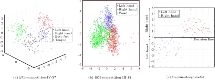
clas-Figure 8. Scatter of feature points output from LDA block. The dimension of LDA projection space is one less than the number of classes. As can be seen, the projected classes are well distinguished: (a) Imaginations of movement of left hand, right hand, both feet, and tongue projected in a three-dimensional LDA projection space, (b) imaginations of movement of left hand and right hand, and generation of words projected in a two-dimensional LDA projection space, and (c)
imaginations of movement of left hand and right hand projected in a one-dimensional LDA projection space. For better visualization, a dummy dimension is added. (best viewed in color).
sied tasks by the proposed method. This gure illustrates the scatter of feature points output from LDA block. Figure 8(a) belongs to subject S7 of BCI competition IV. Because this dataset contains four classes, the dimension of feature vector from LDA output is of three. Figure 8(b) shows the rst subject of BCI competition III, which has three classes. Thus, as it can be seen, features are two-dimensional. Fig-ure 8(c) shows captFig-ured signals. In this dataset, there are two classes, and the dimension of feature vector of LDA output is one. However, for better visualization, the horizontal axis is added as a dummy dimension, which represents the index of samples. As is obvious in this gure, notably high separability between classes has been achieved as a result of optimum blocks used in this method.
6. Signal processing concerns for hardware implementation
In this section, issues relevant to the BCI system performance will be studied. Some parameters, such as the number of lter banks, the number of channels, the number of classes, and the number of features, aect the resulting hardware area. Thus, their values must be known before the hardware design. The dataset used for implementation is the third one (captured signals). 6.1. Number of lter banks
As previously mentioned, the EEG signals must pass the lter banks before applying the SCSSP algorithm. The number of banks should be ecient with regard to both the achieved accuracy and the hardware im-plementation cost. In this case, the number of lters is
chosen to be four, so that these lters can cover alpha (8-12 Hz) and beta (12-16 Hz, 16-20 Hz, 20-24 Hz) frequency bands. The Chebyshev lter with order 6 is used for each lter path.
6.2. Number of classes
Another critical option is to choose the number of classes, inuencing some parameters of LDA and SC-SSP algorithms. In addition, it aects the classica-tion design directly, because the basic SVM is only applicable to binary-class tasks. In order to use the SVM method for classication tasks with more than two classes, one-versus-all or one-versus-one approach can be used. In this study, since the hardware is tested for the third dataset, which contains only two classes, the number of classes of dataset is set to two.
6.3. Number of channels
Another parameter that aects the implementation is the number of channels. This parameter aects the clock rate of the DC-block, Laplacian lter, Chebyshev lter, and SCSSP module. The number of channels is set to 14 in the third dataset.
6.4. Number of features
The number of features, set to 40, inuences the transfer matrix dimension of LDA used to reduce the number of features and SCSSP units, which generate the best features before applying LDA.
7. Hardware implementation
Herein, a two-class case is implemented as an instance of implementation. This implementation can be easily generalized to the case of more than two classes.
Appli-cations of two-class case are very wide, such as moving the head of hospital bed up/down by thinking about movements of right/left hand. This can especially help patients with disabilities in moving body. There are also various applications in smart homes, where turning on and o the electrical devices can be performed by merely thinking about right and left hand movements. In addition, as mentioned in Section 2, recently in the literature, it has been proposed to code several tasks in a state machine using only the right- and left-hand signals [48].
In this work, solely, the testing phase of classi-cation is implemented in hardware, as training can be performed beforehand and there is no need to implement it. The training phase can be done in software such as MATLAB or C language (MATLAB is used in this work), and the resulted coecients can be saved and used for the test phase, which is implemented in hardware.
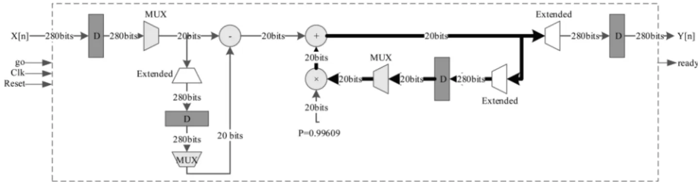
7.1. Implementation of DC-block
The rst block in the proposed BCI system is the DC-block, with the structure, illustrated in Figure 9. As can be seen in this gure, it consists of one adder, one constant multiplier, and one subtractor. Because there are 14 parallel data channels that need to be ltered independently, there is a need for 14 parallel DC-block cores.
In such a situation, by means of applying the folding technique on the multiplier module (i.e., to design the DC-block with only one multiplier for all input channels), the silicon area minimization is en-hanced. This achievement is obtained by sacricing the throughput. However, because of the large sampling frequency of the recording device that is equal to 128 Hz for Emotiv® system, such a decrease in the
throughput can be overlooked. As marked in Figure 9, the critical path of this core consists of only one multiplier and one adder, resulting in the operational frequency of up to 132 MHz, which is fast enough to handle such a low-frequency EEG signal.
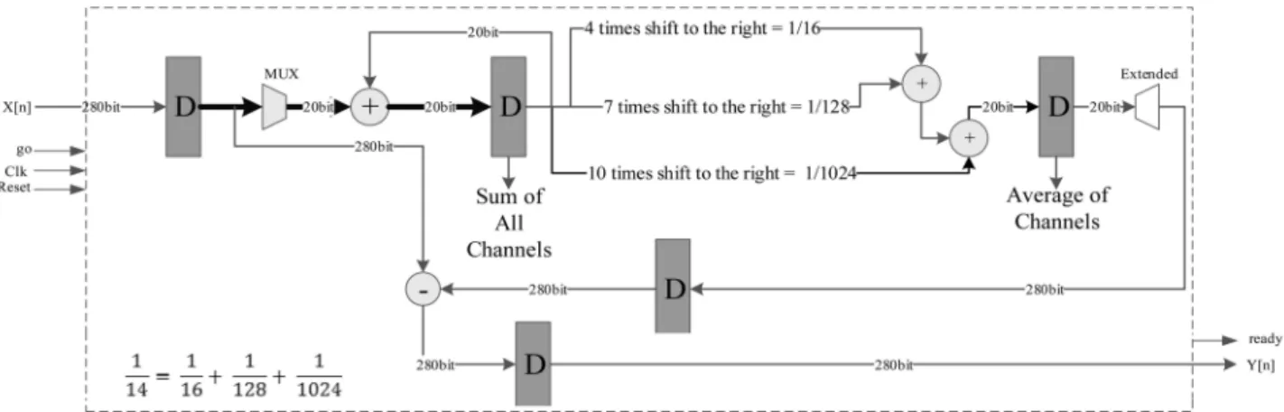
7.2. Implementation of Laplacian lter
As stated in the previous sections, the Laplacian lter is based on the CAR algorithm, in which the mean of all channels is subtracted from all of them. The structure of this core is shown in Figure 10. There is one adder to compute the sum of all channels. The division of the output by the number of channels is realized through simple shift operations. In this way, a signicant area and power can be saved, i.e., 1
14 = 161 + 1
128+10241 = 0:0713. As shown in Figure 10, the critical
path of this module consists of two adders. Therefore, the operation frequency of this module can be up to 234 MHz. The minimum speed of this module with respect to the sampling frequency of 128 Hz can be found based on the following equation: 14
x +x1 +14x in which x is
the minimum limit of the operation frequency, which is 3718 Hz.
7.3. Implementation of Chebyshev lter
Separable Common Spatio-Spectral Patterns (SC-SSP) [30] are used to extract features of motor-imagery tasks. In this algorithm, input data goes through a bank of band-pass lters in the frequency ranges of 8-12 Hz ( band) and 8-12-30 Hz ( band). We have used Chebyshev II band-pass lter of order 6. The block diagram of this lter is illustrated in Figure 11. In this gure, biand aiparameters are the nominator and
denominator coecients of this lter, respectively. It is important to note that this lter can be implemented by means of 12 multipliers (there are two constants and two zero coecients). Each lter bank should be ap-plied to all input channels simultaneously, and it ends up in a number of 168 (12 14) multipliers per lter bank, leading to 672 (4168) multipliers with a bank of four lters, which is not feasible for implementation. In order to overcome this limitation, the folding technique is used between 14 input channels at each lter to reduce the total number of multipliers from 672 to 48 (412), resulting in a signicant reduction in area and power consumption in this module. The critical path of this module consists of two multipliers and seven
Figure 9. Block diagram of the proposed hardware implementation for DC-block. According to Eq. (1), we have Y (z)(z 1 1) + X(z)(1 z 1) = 0. Thus, Y [n 1] Y [n] + X[n] X[n 1] = 0. The left section of gure prepares
Figure 10. Block diagram of the proposed hardware implementation for Laplacian-Filter. Number of channels is 14. The division 1
14 in Eq. (3) is implemented using three simple shift-to-right actions: (161 +1281 +10241 ). The rst adder sums up
the whole channels. The subtraction is for subtracting average from every channel.
Figure 11. Block diagram of the proposed hardware implementation for Chebyshev. The transfer function of this lter can be written as H(z) = Y (z)X(z) =PP6i=0biz i
6 i=0aiz i.
adders; however, it is improved by means of retiming technique to reduce this path to only one multiplier and two adders, resulting in maximum frequency of about 106 MHz. The latency of this module is 99 (1+14(6+1)) clock cycles. Therefore, the minimum limit of the operational frequency in this module should be 12.3 kHz (99 128 Hz).
7.4. Implementation of SCSSP
After applying the proposed band pass lters, the SCSSP [30] core should be applied to the ltered data, in order to extract corresponding features of motor-imagery tasks. The functional structure of this algorithm is summarized in Figure 12. As is shown in this gure, ltered vector X consists of 4 14 elements
Figure 12. Block diagram of the proposed hardware implementation for SCSSP. Stage 1: Implementation of Eq. (8); Stages 2 and 3: implementation of var(yk); Stages 4 and 5: implementation ofPk2Rvar(yk); Stage 6: implementation of
var(yk) P
k2Rvar(yk); Stages 7, 8, and 9: implementation of Eq. (9). Note that the eigenvalues and eigenvectors in this module are
calculated formerly in the train phase though software.
from all 14 channels and 4 lters at a time instance. This vector should be multiplied by the \NewT" matrix that consists of 40 sub-matrices with size of 414 (there are 40 features), whose elements are determined during the train phase of the experiment. The matrix \NewT" is (wR;j[k] wL;i[k])T, where wR;j[k] and wL;i[k] are
the eigenvectors in WR and WL corresponding to j[k]R
and i[k]L , explained in SCSSP section. The result is named \Tmpt" vector, whose elements are squared to construct \Tmpt2" vector. This procedure is repeated after receiving the next sample whose \Tmpt2" vector is added to the previous \Tmpt2". This job is repeated for 3 fs (128 Hz) times. After that, the new
\Tmpt2" vector is decomposed to 2 parts due to the number of classes. Each part of the vector consists of 20 elements. The next step is to sum up these elements so that each part of these vectors is divided by its corresponding sum result. The implementation of the logarithmic function is also implemented by the following equivalency:
Ln(x) = 2Arctanh
x 1 x + 1
: (19)
An overview of dierent stages in SCSSP al-gorithm is marked by means of black hexagons in Figure 12. Each stage is a sub-module and designed to dictate a total critical path of one adder and one multiplier for the whole design, which was made possi-ble using an eective pipelining technique specically in the divider and Arctanh operations, in addition to the folding and retiming techniques used in the design. These eorts resulted in an eective high-speed feature extraction operating at 102 MHz clock speed. The minimum speed of the operational frequency in this module is 560 kHz.
7.5. Implementation of normalization
After feature extraction, the features should be nor-malized. To reach this goal, test features should be subtracted from the average of train features and, then, divided into standard deviation of train features.
Figure 13. Block diagram of the proposed hardware implementation for normalization. Notice that the mean and standard deviation of training data (Eqs. (10) and (11)) are calculated erstwhile in the software and are used here as constant vectors. This gure illustrates the implementation of Eq. (12).
The block diagram of normalization is illustrated in Figure 13. The latency of this module is 40 clock periods. The number of clocks taken to generate output for each feature is 27. Since there are 40 features, it can be concluded that the number of total clocks for this part is 40 27 + 40 = 1120. Therefore, the minimum operational frequency of this module is 1120 128 = 143360 Hz. The maximum speed of this module can be up to 267 MHz.
7.6. Implementation of MI
After normalization, appropriate features should be chosen. Fortunately, this part does not require any hardware. In a training stage, the indices of features are determined. Therefore, according to the index, the corresponding elements of the feature vectors are selected in a test stage. To explain better, the maximum number of features is set to 40, which is found to work for all subjects. In the training phase, mutual information module nds the best indices and the number of features for every subject. This train-ing is performed in software, as explained previously. Then, those elements of transformation matrix (LDA module), corresponding with those numbers of features which are not chosen by mutual information, will be replaced with zeros (masking). Therefore, those numbers of acceptable features are only calculated in LDA module in the testing phase. In the testing phase, a masking process is performed merely in LDA module in order to select the best-found features out of 40 features. Note that, consequently, altering the number of features does not aect the hardware at all. In conclusion, no hardware resources are required to implement mutual information module since the features are selected in the training phase.
7.7. Implementation of LDA
After choosing the best features, their dimension should be reduced. This reduction can be performed by means of the LDA algorithm, which was discussed
previously. In this algorithm, at the train stage, a key matrix is generated. If eigenvectors of this matrix consist of d elements (here, d = 40), then the dimension of this matrix must be (C 1) d, where C is the number of classes. Hence, after multiplying the matrix of selected features by the eigenvectors, the dimension of output vector will be C 1. Herein, due to the classication of left- and right-hand movement motor-imagery tasks, C is equal to 2 and the output is a scalar number. The block diagram of this multiplication is depicted in Figure 14. In this module, the critical path consists of one multiplier and one adder, and the maximum speed of this module can be up to 203 MHz. The latency of this module is 40 clock periods; therefore, the minimum operational frequency of this module should be 5128 (40 128) Hz.
7.8. Implementation of SVM
The last core in the data ow is the classier. This core is designed based on the Linear-SVM algorithm. The main reason for choosing the linear classier is its sim-plicity and eciency in hardware implementation. The block diagram of this core is shown in Figure 15. Based on this gure, the critical path consists of just one mul-tiplier. Therefore, the maximum operational frequency of this module is around 211 MHz. The latency of this module is 2 clock periods; consequently, the minimum limit of the speed of this core is 256 (2 128) Hz.
It is also worth mentioning that implementing non-linear SVM requires adding a non-linear function block to obtain the non-linear function of the dot prod-uct between the support vectors and the test vector. 8. Trade-o of accuracy and hardware
resources
As mentioned before, linear SVM is preferred to Bayesian classier in this work. The detailed compar-ison of these two classiers in terms of performance results and hardware resources is reported in Table 2.
Figure 14. Block diagram of the proposed hardware implementation for LDA. The matrix of eigenvectors has dimension of (C 1) 40 = 1 40, and the input vector X[n] is a 40 1 vector. By multiplying these two vectors, a scalar output is obtained. The multiplication of these vectors is the same as inner product, and the multiplications of elements are accumulated using an adder. Note that the matrix of eigenvectors is obtained formerly through software.
Figure 15. Block diagram of the proposed hardware implementation for Linear SVM. The decision function of SVM is sign(wTx + b) [68], where w's are the weights of SVM, b is the bias, and here x is the output of the previous stage, which
is LDA.
Table 2. Comparison of SVM and Bayesian classiers in terms of performance results and hardware resources. Performance results
S1 S2 S3 S4 S5 S6 S7 S8 S9 Average
BCI competition III (Dataset V, 3 classes)
SVM 86.60% 78.00% 56.00% 73.53%
Bayesian 86.60% 78.00% 61.00% 75.20%
BCI competition IV(Dataset 2a, 4 classes)
SVM 79.20% 56.30% 87.50% 63.90% 41.00% 46.90% 81.90% 76.00% 72.20% 67.21% Bayesian 80.55% 60.10% 87.50% 67.70% 42.70% 46.20% 82.30% 78.10% 74.00% 68.79% BCI competition IV
(Dataset 2a, 2 classes)
SVM 91.67% 59.72% 95.83% 77.08% 67.36% 69.44% 78.47% 97.22% 88.19% 80.55% Bayesian 90.27% 59.72% 95.83% 78.47% 67.36% 69.44% 77.08% 97.22% 90.00% 80.59% Captured signals SVM 93.60% 93.60% 96.80% 83.90% 71.00% 71.00% 58.00% 87.1 0% 81.87%
Bayesian 93.60% 93.60% 96.80% 83.90% 71.00% 71.00% 58.00% 87.10% 81.87% Hardware resources
Add/
Sub Multp Divider Arctan Sinh/Cosh
Latency (clocks)
Power
(mW) LUTs Registers
Captured signals SVM 1 1 0 0 0 2 4.69 63 21
Table 3. The settings of points (experiments) in the Pareto optimal graph shown in Figure 16. Point DC
block Laplacian SCSSP Normalization MI LDA
SVM/ Bayesian
Accuracy (%)
Power (mW)
1 p p p p p p SVM 81.9% 83.00
2 p p p p p SVM 75.5% 85.34
3 p p p p p SVM 77.9% 79.49
4 p p p p p SVM 77.5% 67.80
5 p p p p SVM 75.2% 70.14
6 p p p p SVM 76.0% 73.65
7 p p p p SVM 75.5% 78.32
8 p p p SVM 75.2% 75.99
9 p p p p p p Bayesian 80.8% 90.01
10 p p p p p Bayesian 76.7% 94.69
11 p p p p p Bayesian 76.4% 87.68
12 p p p p p Bayesian 77.1% 80.66
13 p p p p Bayesian 74.0% 86.51
14 p p p p Bayesian 73.9% 78.32
15 p p p p Bayesian 76.7% 75.98
16 p p p Bayesian 74.0% 78.32
As can be seen in this table, the Bayesian classier slightly outperforms linear SVM in accuracy, while its hardware resource usage is signicantly higher and is also much slower than SVM, making it not suitable for motor imagery systems in which fast decision-making is crucial. The very small improvement in accuracy while causing a signicant increase in hardware usage and latency is not encouraging. Moreover, note that power is one of the main concerns in BCI systems fullled by choosing linear SVM over Bayesian classier. Nev-ertheless, one can prefer better accuracy if hardware usage is not an important issue.
For showing the trade-o between accuracy and hardware resources better, dierent permutations of settings are experimented by excluding/including the parts from/in the proposed system. The classica-tion accuracy as well as the consumed power of the experiments are reported by a Pareto optimal graph illustrated in Figure 16. The settings of dierent experiments (points) in this gure are listed in Ta-ble 3. Experiments 1 and 9 in this Pareto optimal graph are the experiments detailed in Table 2. The Pareto optimal graph clearly shows that there exists a trade-o between classication accuracy and hardware eciency, and some settings are the best ones among the possible settings. As can be seen in Figure 16, experiments 1, 3, and 4 are the Pareto optimal points from which the setting of experiment 1 is chosen as the nal setting in this paper, because accuracy is important in our goal.
9. Hardware results
In order to capture, analyze, and process the captured data, the following interfaces and tools are used. The
Figure 16. The Pareto optimal graph for reporting the trade-o between accuracy and power. The settings of the points are listed in Table 3. The red points connected with the green lines are the Pareto optimal points.
utilized evaluation board is Virtex-6 FPGA ML605 Evaluation Platform to which the input data is sent via an Ethernet port. The output signal is tracked and analyzed by Xilinx ChipScope software. The synthesis and analysis of HDL designs are performed using ISE Xilinx 14.5 software. The results of xed-point numbers show that 20 bits are enough for each value of every channel in a way that 11 bits are considered for the decimal part, 8 bits for the integer part, and one
last bit for the sign bit. Thus, the number of bits for one test vector is 280 (14 channels 20). A new test vector is processed every 0.0078s (fs= 128 Hz). Since
each person requires three seconds to perform a given task (see Figure 3), then the number of test vectors for each experiment is equal to 384 (3 128). Each person performs 30 experiments including 15 experiments for the rst class and 15 experiments for the second class (in our captured dataset).
Retiming and folding techniques were used by sacricing the speed, which is justiable because of low sampling frequency of signal recording. Final structure satises maximum frequency of 102 MHz and minimum frequency of 560 kHz, according to Table 4. Table 4 shows the number of Adders, Subtractors, Multipliers, Dividers, and Arctan modules used in the proposed BCI, showing the importance of using folding and
retiming techniques. Note that, for multiplications, Xilinx multiplication cores (LogiCORE IP Multiplier v11.2), which are optimized according to inputs of the core, are utilized. The hardware latency and power of each section and the total framework are also reported in Table 4. Moreover, as seen in Table 4, a wide range of allowed frequencies is provided in this proposed system, helping to increase frequency and have a satisfying and acceptable total latency even in a large number of channels.
The hardware resource usage is reported in Ta-ble 5. It can be seen that the total power of this work, i.e., 83.90 mW, is much less than the total power in [48], which is 1.067 W. As reported in this table, the proposed system outperforms [47] and [48] signicantly in terms of the number of LUTs, the number of block RAM/FIFO, the total latency, and the utilized power.
Table 4. Features of sections of the framework. The rst two columns report the valid operational frequency of the proposed BCI. The next four columns represent the detailed resources utilized in dierent sections. The last two columns display latency and power, respectively. Note that the total latency is the spent time started at the end of motor imagery (which is the 6th second according to Figure 3) and ended when prediction becomes ready. In this table, N and D respectively denote the number of channels and features.
Min. (Hz)
Max. (Hz)
Add/
Sub Multp Divider Arctan Latency
1 Power
(mW)
DC-block 1792 132M 2 1 0 0 14=N 7.44
Laplacian lter 3718 234M 4 0 0 0 18=N +4 1.70
Chebyshev lter 12.3K 106M 4 11 4 12 0 0 99=7N +1 54.15
SCSSP 560K 102M 5 2 0 1 4375=4ND+50D+135 22.04
Normalization 143360 267M 1 0 1 0 1120=27N +40 12.61
MI { { 0 0 0 0 0 0
LDA 5128 203M 1 1 0 0 40=D 7.99
SVM 256 211M 1 1 0 0 2 4.69
BCI (total system) 560K 102M 58 53 1 1 5668=182+36N +51D+4ND 83.90
1Numbers of this column are in clock numbers. The minimum and maximum clock frequencies are reported in the two rst columns.
Notice that identical clock frequency (560 kHz f 102 MHz) is used in the sections of nal setup. The latency can be obtained in milliseconds according to selected clock frequency (10 milli-seconds in the worst case and 55.5 micro-seconds in the best case).
Table 5. Hardware resource usage. The proposed framework outperforms [47] in number of lookup-tables and block RAM/FIFO and cost of a few additional DSP blocks. It also outperforms [48] in number of block RAM/FIFO.
LUTs Block
RAM/FIFO
DSP block
Latency (ms)1
Power (W)1
This work 11,311 65,536 24 10 0.083
[47] 17,281 557,332 4 57776.066 {
[48] 27,906 818,624 644 399 1.067
1The numbers of channels in the hardware implementation are 14, 22, and 22
in this work, [47], and [48], respectively, and the reported latency and power in this table are set according to these settings. However, note that, according to Table 4, latency of the proposed system would be 6534 (1=560 kHz) 11:66 ms for N = 22 channels much better than in [47] and [48]. In addition, as explained in paragraph 3 of Section 9, the hardware is not altered signicantly by changing number of channels; therefore, power does not signicantly change, too.
It outperforms [48] in the number of DSP blocks, too. The reason of outperforming [48] in the number of DSP blocks and multipliers is having lters with order six, while the order of lters increases signicantly (to, e.g., 221 and 442) to achieve higher accuracy. On the other hand, the proposed system outperforms [48] in terms of block RAM/FIFO which is because most of the tuned and trained parameters saved in our system are scalars (e.g., in SVM) or vectors (e.g., in LDA) and merely one matrix saved for SCSSP. However, more matrices are required to be saved in [48], which are the matrices needed for CSP section and covariance matrix in Mahalanobis distance. Moreover, folding and retiming techniques help our system have better power consumption and area. Paper [47], although has the lower performance rate (72%) on BCI Competition IV dataset (2 classes), its latency is not completely proper for practical applications.
Note that, in the proposed system, changing the number of channels does not alter the utilized hardware resources too much because normalization, SVM, and LDA structures are independent of the number of the channels, and merely some wires and bits in registers are added in DC-block, Laplacian lter, Chebyshev lter, and SCSSP. Consequently, the number of RAM/FIFO and DSP blocks do not change, while the number of LUTs blocks increases a little and not signicantly.
10. Conclusion
This paper proposed an ecient hardware imple-mentation for BCI systems. The proposed system consists of preprocessing, feature extraction, feature selection, feature reduction, and classication stages. Software simulations and hardware limitations guided the method to choose DC-block and surface Laplacian as preprocessing, SCSSP as feature extractor, MI as feature selector, LDA as feature reduction method, and SVM as classier. Results determined the proper performance of the proposed system, compared to other reported results on the used datasets (67.2% for BCI competition IV, 73.54% for BCI competition III, and 81.9% for captured signals). The system was also e-ciently implemented and tested on a FPGA hardware platform. The minimum frequency of BCI system was 560 kHz. Moreover, because of using Folding and Retiming techniques, the number of resources (LUTs and block RAM/FIFO) decreased dramatically, on cost of a few additional DSP blocks.
Blinking can have destructive impact on the obtained accuracy. By using an appropriate EOG detection during the mental task, it is possible to increase the signal-to-noise ratio and, thus, accuracy. Moreover, in all these experiments, it was known when the subjects were going to do the mental task.
Predicting when subjects are going to think about the task by extracting ERD/ERS features can be added to the proposed framework (see Section 3.3 of [69]). References
1. Wolpaw, J.R., Birbaumer, N., McFarland, D.J., Pfurtscheller, G., and Vaughan, T.M. \Brain-computer interfaces for communication and control", Clin. Neurophysiol., 113(6), pp. 767-791 (2002).
2. Duchowski, A.T., Eye Tracking Methodology: The-ory and Practice, Springer International Publishing AG, 3rd Ed., ISBN 319-57881-1, ISBN 978-3-319-57883-5 (eBook) (2017). DOI 10.1007/978-3-319-57883-5
3. Ferracuti, F., Freddi, A., Iarlori, S., Longhi, S., and Peretti, P. \Auditory paradigm for a p300 BCI system using spatial hearing", In Intelligent Robots and Systems (IROS), 2013 IEEE/RSJ International Conference on, IEEE, pp. 871-876 (2013).
4. Kathner, I., Ruf, C.A., Pasqualotto, E., Braun, C., Birbaumer, N., and Halder, S. \A portable auditory P300 brain-computer interface with directional cues", Clinical Neurophysiology, 124(2), pp. 327-338 (2013).
5. Kim, D.-W., Hwang, H., Lim, J.-H., Lee, Y.-H., Jung, K.-Y., and Im, C.-H. \Classication of selec-tive attention to auditory stimuli: toward vision-free braincomputer interfacing", Journal of Neuroscience Methods, 197(1), pp. 180-185 (2011).
6. Pfurtscheller, G., Brunner, C., Schlogl, A., and Da Silva, F.H.L. \Mu rhythm (de) synchronization and EEG single-trial classication of dierent motor im-agery tasks", NeuroImage, 31(1), pp. 153-159 (2006).
7. Khurana, K., Gupta, P., Panicker, R.C., and Kumar, A. \Development of an FPGA-based real-time P300 speller", 22nd International Conference on Field Pro-grammable Logic and Applications (FPL), Oslo, pp. 551-554 (2012).
8. Xu, B., Song, A., and Wu, J. \Algorithm of imag-ined left-right hand movement classication based on wavelet transform and AR parameter model", Bioinformatics and Biomedical Engineering, The 1st International Conference on. IEEE (2007).
9. Schlogl, A., The Electroencephalogram and the Adap-tive Autoregressive Model: Theory and Applications, Germany: Shaker (2000).
10. Pfurtscheller, G., Neuper, C., Schlogl, A., and Lugger, K. \Separability of EEG signals recorded during right and left motor imagery using adaptive autoregressive parameters", in IEEE Transactions on Rehabilitation Engineering, 6(3), pp. 316-325 (Sept. 1998).
11. Schlogl, A., Lugger, K., and Pfurtscheller, G. \Us-ing adaptive autoregressive parameters for a brain-computer-interface experiment", Proceedings 19th In-ternational Conference IEEE/EMBS (1997).
12. Dharmasena, S., Lalitharathne, K., Dissanayake, K., Sampath, A., and Pasqual, A. \Online classication of