Multiple layer image analysis for video microscopy

(1)

Multiple Layer Image Analysis for Video Microscopy

Brian S. Eastwood

A dissertation submitted to the faculty of the University of North Carolina at Chapel Hill in partial fulfillment of the requirements for the degree of Doctor of Philosophy in the Department of Computer Science.

Chapel Hill 2009

Approved by:

Russell M. Taylor II, Advisor

Marc Niethammer, Reader

Gary Bishop, Reader

Leonard McMillan, Committee Member

(2)

(3)

Abstract

Brian S. Eastwood: Multiple Layer Image Analysis for Video Microscopy. (Under the direction of Russell M. Taylor II.)

Motion analysis is a fundamental problem that serves as the basis for many other image analysis tasks, such as structure estimation and object segmentation. Many motion analysis techniques assume that objects are opaque and non-reflective, asserting that a single pixel is an observation of a single scene object. This assumption breaks down when observing semitransparent objects—a single pixel is an observation of the object and whatever lies behind it. This dissertation is concerned with methods for analyzing multiple layer motion in microscopy, a domain where most objects are semitransparent. I present a novel approach to estimating the transmission of light through stationary, semitransparent objects by estimating the gradient of the constant transmission observed over all frames in a video. This enables removing the non-moving elements from the video, providing an enhanced view of the moving elements.

I present a novel structured illumination technique that introduces a semitranspar-ent pattern layer to microscopy, enabling microscope stage tracking even in the presence of stationary, sparse, or moving specimens. Magnitude comparisons at the frequencies present in the pattern layer provide estimates of pattern orientation and focal depth. Two pattern tracking techniques are examined, one based on phase correlation at pat-tern frequencies, and one based on spatial correlation using a model of patpat-tern layer appearance based on microscopy image formation.

Finally, I present a method for designing optimal structured illumination patterns tuned for constraints imposed by specific microscopy experiments. This approach is based on analysis of the microscope’s optical transfer function at different focal depths.

(4)

(5)

Acknowledgments

There are many people to whom I am grateful for their help in completing this dissertation. I thank my advisor, Russell Taylor, for working closely with me over the past six years and for providing encouragement and clarity when I needed it. I will miss our many hours of brain hurting math.

I consider myself very fortunate to have had the support of my committee members, Marc Niethammer, Gary Bishop, David Hill, and Leonard McMillan. They have provided a wealth of guidance and insight throughout my graduate career. I thank Richard Superfine for—along with Russell—fearlessly leading CISMM, for helping me understand Fourier optics, and for providing very helpful and constructive criticism. My thanks go to Mary Whitton for being a strong mentor to me, helping me with my writing, and providing guidance in teaching. I also extend special thanks to Lamar Mair for creating the test square grid patterns used throughout this work.

This work was funded in part by the National Institute of Biomedical Imaging and Bioeni-neering (NIBIB), grant number P41-EB002025.

The staff of the Computer Science department at UNC are second to none. I thank them all for their help over the years.

I have many friends, collaborators, and colleagues at UNC and beyond who have influenced my work and provided encouragement. They are Jill Aldredge, Rob Aldredge, Brian Austin, Greg Baker, Amanda Baltzley, Michael Baltzley, Eric Bennett, Aaron Block, Kerry Bloom, David Borland, Fred Brooks, Sabrina Burmeister, Samuel Caro, Brianna Carstens, Mukta Chakraborty, Diana Clark, Jeremy Cribb, Kyla Davidoff, Edward Dale, Ben Evans, Mike Falvo, David Feng, Yoni Friedman, Matt Fuxjager, Nico Galoppo, Guido Gerig, Casey Goodlett, Nathan Hudson, Melanie Kessels, Bill Kier, Anselmo Lastra, Christina Lebonville, Steven Lebonville, Cathy Lohmann, Kenneth Lohmann, David Marshburn, Bruce Maxwell, Justin McAlister, Suzanne McAlister, Daniel Millard, Tim O’Brien, Angela Oyeno, Ted Oyeno, Justin Peters, Stephen Pizer, Marc Pollefeys, Rebecca Price, Cory Quammen, Danielle Racke, Jenny

(6)

Rice, Ted Salmon, Katrina Salvante, Jason Sewall, Kendra Sewall, Ryan Schubert, Adam Shields, Montek Singh, Dale Skrien, Jack Snoeyink, Keith Sockman, Ricky Spero, David Stotts, Vinay Swaminathan, Stephanie Taylor, Scott Taylor, Jur van den Berg, Leandra Vicci, Sean Washburn, Stephen Weiss, Jeremy Wendt, Buddy Whitman, Brian Wilson, Shun Xu, and many others.

I am eternally grateful to my parents, Abe Eastwood and Judy Brook, who have instilled in me the passion for lifelong learning and provided me with many opportunities and experiences. My father taught me how to write my first computer program. My mother spent summers teaching me about the natural sciences. I also thank Sutton Monro, Jo Ann DiMartini, and Anne and Vinnie Mangiamele, for their love and support. I thank my brother, Chuck, for being the big brother I always look up to. I thank Suzanne and Carl Eastwood for keeping me smiling.

(7)

List of Tables

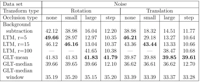
4.1 Mean PSNR measurements for repairing simulated microscopy data. . . . 61

5.1 Phase estimation using DFT and WPC, pure signal . . . 94

5.2 Phase estimation using DFT and WPC, corrupted signal . . . 96

5.3 Tracking error for different noise models . . . 101

5.4 Tracking error for varying orientation and translation . . . 105

5.5 Tracking error for experimental and simulated images . . . 117

5.6 Tracking error for experimental and simulated images with specimen . . . 120

(13)

List of Figures

2.1 Bright-field microscope optical path. . . 11

2.2 Image formation by a thin lens . . . 13

2.3 Numerical aperture of a microscope objective lens . . . 15

2.4 Diffraction of light through an aperture . . . 18

2.5 A simulated point spread function. . . 21

2.6 The XZ plane of the microscope point spread function. . . 22

2.7 A flat-field calibration image . . . 32

2.8 Gain calibration for a CCD image sensor . . . 35

4.1 Ciliated epithelial lung cells move a bead . . . 48

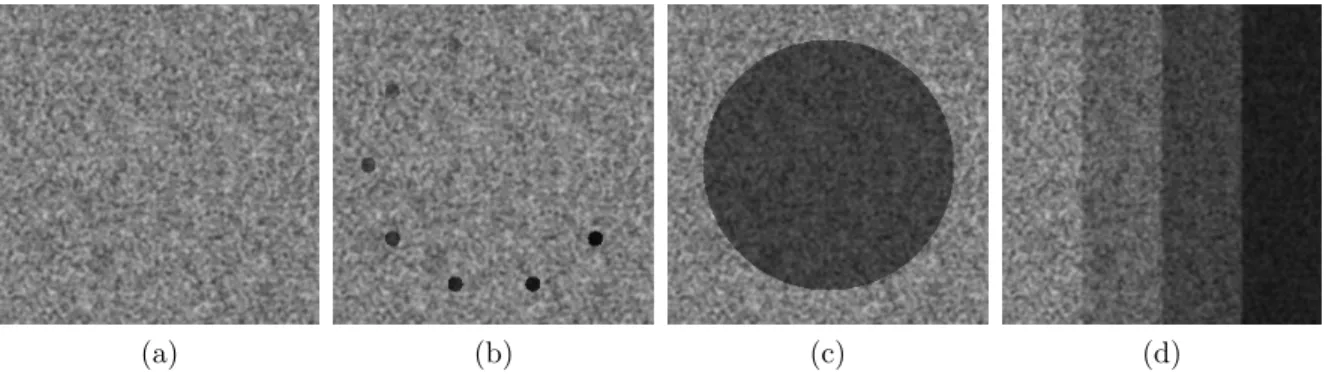
4.2 Sample test data of transforming noise fields. . . 60

4.3 Transmission maps recovered from step function occlusion. . . 62

4.4 Repair of cilia microscopy video. . . 64

4.5 Stationary occlusion removal applied to cilia culture. . . 65

4.6 Occlusion removal before flow computation . . . 67

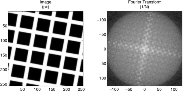
5.1 A square grid pattern and its Fourier transform . . . 74

5.2 Finding the orientation of a regular grid . . . 75

5.3 Discrete Fourier transform of single-frequency sinusoids. . . 85

5.4 Weighted phase correlation in 1D . . . 89

5.5 Weighted phase correlation in 2D. . . 90

5.6 Comparison of phase estimation using DFT and WPC, pure signal . . . . 94

5.7 Comparison of phase estimation using DFT and WPC, corrupted signal . 96

(14)

5.8 Grid pattern image simulation. . . 98

5.9 Mean displacement error for different noise models. . . 100

5.10 Orientation error using frequency and model-based estimates . . . 103

5.11 Translation error with different pattern rotations . . . 104

5.12 Tracking error for small translations . . . 106

5.13 Simulated grid with varying transmissions. . . 106

5.14 Tracking error for varying transmission . . . 107

5.15 Simulated square pattern at different depths . . . 108

5.16 Tracking error for varying focus . . . 109

5.17 Effect of transmission and focus on orientation estimation . . . 110

5.18 Measuring optical transmission from images . . . 115

5.19 Experimental images of a square grid micropattern . . . 116

5.20 Octopus muscle and micropattern . . . 118

5.21 Experimental and simulated microscopy images . . . 120

5.22 Microscopy mosaic image of octopus muscle . . . 123

6.1 Microscope optical transfer function . . . 134

6.2 Optimal frequency selection . . . 138

6.3 Focus estimation from model fitting. . . 143

6.4 Effect of pattern spacing on tracking error . . . 145

6.5 Predicted SNR for pattern optimized for a sparse specimen . . . 149

6.6 Tracking error in the presence of a sparse specimen . . . 150

6.7 Predicted SNR for pattern optimized for frog brain tissue . . . 152

6.8 Tracking error in the presence of frog tissue . . . 153

(15)

6.10 Focus error with specimen present, 40X objective . . . 155

6.11 Focus error for non-optimized pattern . . . 156

6.12 Focus error with specimen present, 20X objective . . . 157

A.1 ImageTracker main window . . . 168

A.2 ImageTracker load image panel . . . 170

A.3 ImageTracker vector visualizations . . . 173

A.4 Applying the threshold filter . . . 175

A.5 Gaussian and gradient filters . . . 176

A.6 Flat-field filter . . . 178

A.7 Fluorescent labeling of a mitotic spindle . . . 184

(16)

List of Abbreviations

1D . . . one-dimensional

2D . . . two-dimensional

3D . . . three-dimensional

ADC . . . analog-to-digital converter

CCD . . . charge-coupled device

CISMM . . . Computer Integrated Systems for Microscopy and Manipulation

DC . . . direct current, mean amplitude

DFT . . . discrete Fourier transform

DIC . . . differential interference contrast

EM . . . electromagnetic

GLT . . . gradient logarithm transmission

GUI . . . graphical user interface

ITK . . . Insight Toolkit

LTM . . . local transmission metric

MCL . . . Mad City Labs

MSC . . . model-based spatial correlation

NA . . . numerical aperture

NCC . . . normalized cross-correlation

NIH . . . the National Institutes of Health

OTF . . . optical transfer function

OTL . . . optical tube length

(17)

PSNR . . . peak signal-to-noise ratio

RANSAC . . . random sample consensus

RMS . . . root mean squared

SNR . . . signal-to-noise ratio

TEM . . . transmission electron microscope

UNC . . . the University of North Carolina at Chapel Hill

USD . . . United States Dollars

VTK . . . Visualization Toolkit

WPC . . . weighted phase correlation

(18)

List of Symbols

cm . . . centimeter, 10−2 meters

Cr . . . chromium

dB . . . decibel

◦ _{. . . degrees}

fps . . . frames per second

Au . . . gold

µm . . . micrometer or micron, 10−6 _meters

µs . . . microsecond, 10−6 seconds mm . . . millimeter, 10−3 _meters

nm . . . nanometer, 10−9 meters

(19)

Chapter 1 Introduction

This dissertation considers analysis of images formed of scenes containing multiple

semi-transparent objects. The goal of image analysis is to extract information from images

that provide insight about the scene, such as the size, shape, and motion of objects in

it. Models of image formation drive the image analysis process by providing constraints

that inform the researcher about how an object will appear when imaged.

A great deal of image analysis research considers objects to be opaque and non-reflective, such as a piece of clay. In an image of such an object, the information at a

single image location comes from a single point on the object. The situation changes,

however, when imaging semitransparent objects, such as frosted glass. In an image of

such an object, a single image location contains information from the semitransparent

object and whatever lies behind it. Under these conditions, different models of image

formation are required to form accurate insight about the scene being observed.

Multiple layer imaging presents a combination of challenges and opportunities. Many

image analysis techniques established for images of opaque objects break down in the mixture of information from multiple layers. The benefit of semitransparency, however,

is that an object is visible at all times, even when hidden behind another object. This

means there is information about the object in the image—the trick is getting at it.

(20)

of biological specimens at the microscopic scale, transparency is the norm—small fish,

worms, parameciums, cell membranes, organelles, and cellular scaffolding are all

com-ponents of a semitransparent world of great interest to science.

My thesis statement is:

Tracking multiple, semitransparent, moving layers in microscopy videos

requires image analysis techniques that are different from those used in

tracking opaque objects. Median gradient estimation of log-intensity

im-ages enables the accurate removal of the stationary component from videos

containing semitransparent moving objects. Harmonic analysis of

struc-tured illumination pattern frequencies and model-based spatial correlation enable three dimensional stage tracking for microscopy. Semitransparent

patterns composed of optimally-selected sinusoids enable tracking with

ac-curacy below the Abbe resolution limit.

The thesis statement is examined in the context of the following novel results of this research:

• I present a novel technique for recovering a model of stationary objects in multiple layer images [ET07].

– Median gradient estimation of log-intensity images yields an estimate of the constant gradient of light transmitted through each location in a series of

bright-field microscopy images. A Fourier transform-based gradient

integra-tion constructs a model of the staintegra-tionary light transmission field.

– This model provides a specimen-specific field correction that removes station-ary components from the images.

(21)

• I present a novel structured illumination technique that introduces a semitrans-parent image layer to microscopy images to provide stage tracking information

even in the presence of stationary and moving specimens.

– Magnitude comparisons at the frequencies present in the pattern layer provide estimates of pattern orientation and focus depth.

– Two pattern-layer tracking techniques are examined, one based on phase correlation and one on spatial correlation.

– The phase correlation approach could be fast enough for online tracking, and is accurate to within 0.01 pixel for unoccluded light paths and within 0.2

pixel in the presence of moving semitransparent specimens with

sparsely-distributed contrast at focal distances up to 6 times the depth of field of the

objective lens.

– The spatial correlation approach is accurate to within 0.5 pixel in the presence of a moving semitransparent specimen that has densely-distributed contrast.

– Analysis of the microscope objective optical transfer function (OTF) enables optimal pattern design of sinusoidal patterns tuned for specific microscopy

experiments.

1.1 Microscopy Applications

The techniques developed in this research are applicable to a broad range of microscopy

imaging applications. The following represents a brief overview of active research that

may benefit from my research.

(22)

Cilia-driven flow

Ciliated human epithelial lung cells are grown from tissue culture in glass chambers to

study the dynamics of cilia-driven mucus flow [BB08]. In experiments performed by

some of my collaborators at the University of North Carolina at Chapel Hill (UNC), an

inverted light microscope focuses on the cilia or into the mucus layer at the top surface of the cells, through the bottom of the container, the cell substrate, and the cell bodies.

The thickness of the cell layer is approximately 10µm, the cilia layer is 7µm, and the mucus layer is up to 50µm. A long working distance lens is required to focus this far into the specimen, and subsequently the image formed has a large depth of field. Visible

within one image are the fixed cell structures, the beating cilia, and particles in the

flowing mucus layer.

Stationary occlusion removal, discussed in Chapter 4, processes such videos to ex-clude the non-moving cell layer, enhancing the motion at the cilia and mucus layers.

Ongoing research is concerned with observing mucus flow over regions spanning

multi-ple fields of view. Structured illumination microscopy would provide a method to track

the stage motion, establishing the relative position of different observations with the cell

culture.

Vesicle transport

Intracellular vesicle transport occurs along microtubules—cell scaffolding structures—

driven by molecular motor proteins such as kinesin and dynein [HPBH04]. Transport

along 100−200µm neurites that are fixed to the top surface of a cover slip are imaged with a 60X, 1.0NA water immersion lens and images are acquired with a 55×55µm2_field

of view. Vesicle motion up to 15µm is tracked using differential interference contrast (DIC) microscopy with background subtraction from a computed sliding mean of images.

My occlusion removal method may enhance the view of vesicle transport in

(23)

longer ranges, across multiple fields of view or even along pathways oblique to the image

plane.

Bead diffusion

Diffusion experiments investigate the motion of small particles—for example, polystyrene

microbeads—through liquids of different concentrations (such as sucrose),

semiperme-able membranes (such as cell and nucleus membranes), and meshes (such as fibrin protein

clots). Current experiments are constrained to 200µm fields of view, observed with a 40X lens (Tim O’Brien, personal correspondence). Structured illumination microscopy

may enable observations in such experiments over long ranges with an understanding of

how far from the seed location beads have diffused.

Cell motility

Cell motility research seeks to understand the mechanics of cell motion. Observed over a long period of time, some cells migrate long distances, alternately extending filopodia

and contracting the cell body. Typical cell bodies are approximately 10µm thick (Tim O’Brien, personal correspondence). Structured illumination microscopy may provide a

way to track individual cells over many fields of view, maintaining accurate information

about total cell motion.

Sea urchin larvae development

Research comparing the evolution of larvae development in related populations of Pacific

and Caribbean sea urchins involves making three-dimensional (3D) measurements of

larva arms using bright-field microscopy [McA08]. In this research, lateral (x and y)

positions are recorded using a camera lucida, which enables simultaneously viewing the microscope field and a digital drawing tablet. The axial (z) positions are obtained

(24)

through coupling the microscope’s fine focus knob to an optical encoder. Measuring

distances of 240µm in 3D is typical in this research. Structured illumination may provide a method to measure these 3D distances more directly.

Nematode tracking

Nematodes are small, semitransparent worms used in research of chemical,

mechani-cal, and thermal sensing and motion regulation. Recent research has concentrated on

effective methods to track the sinusoidal motion of these specimens over long ranges,

but this is often constrained to the field of view of the imaging system [TT07]. Low

magnifications are used to track populations of the worms within a wide field [HS06],

and motorized microscope stages provide tracking of individual animals at higher res-olutions [GCB+_{04]. Structured illumination microscopy may provide tracking at high}

magnifications without the use of motorized stages.

Combined fluorescent and bright-field microscopy

Fluorescent dyes stain cellular structures, such as actin or tubulin, so that they are visible

with a fluorescent microscope, but not with transmitted light illumination (bright-field).

Most fluorescent microscopes also have bright-field capabilities, and some microscopes

enable switching quickly between the two modes [SSW+_{03]. With such a setup, moving}

structures could be observed in fluorescence and tracked using structured illumination

microscopy.

1.2 Outline

The remainder of this dissertation is organized as follows. Chapter 2 provides an

(25)

tech-nique for removing stationary, semitransparent image layers from microscopy videos.

Chapter 5 discusses two techniques for determining the lateral motion of

semitranspar-ent patterns and the application to tracking a microscope stage. Chapter 6 discusses

the design of patterns optimized for structured illumination microscopy tracking, and

extends stage tracking to three dimensions. Chapter 7 summarizes the dissertation and

presents avenues for future research in this field.

(26)

Chapter 2 Microscopy Image Formation and

Acquisition

As mentioned in Chapter 1, this work is concerned with analyzing information from

multiple mixed image layers. Multiple layer images arise often in biological microscopy

where the objects under study are semi-transparent and a non-zero depth of field means

images are formed of objects from multiple levels in the specimen. Before examining how

to extract layer information from microscopy images, it is necessary to understand how microscopy images are formed. In this chapter I will discuss the optics of microscopy

image formation, digital image acquisition, and image sensor noise characteristics.

The fundamental concern in image acquisition is the behavior of light. Visible light

is a thin spectrum of electromagnetic (EM) radiation. EM radiation is a transverse

wave phenomenon—the radiation propagates in one direction and a pair of orthogonal

electric and magnetic fields oscillate tangential to the propagation direction [Mur01, Ch.

2]. The EM waves in visible light have wavelengths between 400 and 700 nm. The speed of light propagation is constant for all wavelengths, but depends on the medium through

which the light is passing:

v =λf, (2.1)

(27)

and frequency of the light wave, respectively.

Like many natural phenomena, several models exist to explain how light behaves,

and each model is appropriately applied at different scales of observation. In free space,

light waves travel in a straight line and parallel light waves remain parallel, like waves

across the open ocean. At large scales, light can be modeled as traveling in straight

rays. This is the domain of geometrical optics analysis, which can be used to describe

image magnification in lenses. In computer graphics, ray tracing is an application of

geometrical optics analysis.

When light is obstructed by a barrier, the light waves bend—diffract—spread out on

the other side of the barrier, like ocean waves passing through a breakwater in a harbor.

Though light diffracts in all optical systems, the diffraction effect is more apparent for

smaller apertures, especially for apertures smaller than several wavelengths of the light.

This is the domain of Fourier optics, which considers the propagation and interference

of EM waves. Macroscale photography can often accurately model image formation by

considering only the ray behavior of light, but microscopy imaging requires considering the effects of diffraction.

The energy in EM radiation is carried in quantized packets called photons. When

light is incident on a surface, such as certain metals, the photons can interact with

electrons in the material. This is the domain of quantum physics, which considers the

particle nature of light. This atomic-scale phenomenon is fundamental to the operation

of digital image sensors.

The quantum theory of light—specifically quantum electrodynamics—is consistent in describing the behavior of light at the diffraction and macroscopic scales; Fourier

optics theory is consistent in describing behavior at the macroscopic scale. Each larger

scale theory, however, offers simplifications that make analysis easier at each of the

different scales. In the sections that follow, I will rely on each of the light models to

build a complete explanation of how images are formed and captured in digital video

(28)

microscopy.

2.1 Microscope Optics

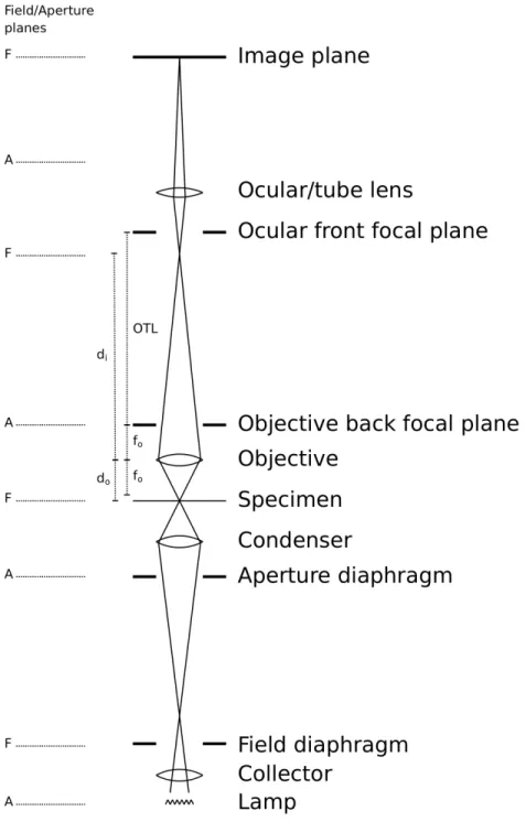
In bright-field microscopy, light passing through a specimen is collected and focused by a series of lenses to form an image of the specimen at the image sensor plane. Figure 2.1

diagrams the major components of a bright-field microscope. Bright-field microscopes

share a common optimal lens alignment scheme—known as K¨ohler 1 _alignment_—with

several types of light microscopes,e.g. dark-field, phase contrast, differential interference

contrast, and fluorescence [Mur01, Ch. 1]. Each of these imaging modalities relies on a

different property of light to generate contrast, and a single microscope can often switch

among these different modes.

Understanding how images are formed in a microscope requires knowledge of its

optical alignment. This provides a basis for understanding what effect different elements

in the microscope light path have on the images formed. K¨ohler alignment, introduced

by August K¨ohler in 1893, specifies how to position the lenses in a microscope in order to

create two conjugate sets of image planes. Field planes are locations where the specimen

is in focus. Aperture planes are locations where the illuminating lamp is in focus. Light

from the lamp is completely out of focus at the specimen plane, providing a uniform illumination field. K¨ohler alignment provides two major benefits:

1. Uniform specimen illumination. In an alternative illumination scheme—one used

on microscopes before 1893—an image of the light source is focused on the

speci-men plane, confounding understanding of the specispeci-men structure.

2. Independent adjustment of numerical aperture (NA) and field of view. The NA

controls the quantity of light collected by the objective lens and determines the

(29)

Figure 2.1: The optical path of a bright-field microscope. Light rays (straight lines) intersect at the field planes, where the specimen is in focus. The specimen is placed slightly in front of the front focal plane of the objective lens, which projects a magnified intermediate image in the microscope top tube. The ocular lens further magnifies this image to form an image at the image observation plane.

(30)

resolution limit of the microscope. The field of view determines the area of the

specimen that is illuminated.

The aperture light path forms focused images of the illumination lamp at several

points in the microscope’s optical path. The collector lens focuses light from the lamp

onto the aperture diaphragm. Adjusting the aperture diaphragm changes the angle of

the cone of light that illuminates the specimen, which affects contrast and resolution. In

practice, the aperture diaphragm is usually left fully open. The condenser lens defocuses the lamp image at the aperture diaphragm into parallel rays at the specimen plane,

providing uniform illumination across the field of view (the image of every point on the

lamp is spread out over the specimen plane). The objective lens creates a focused image

of the lamp at the back focal plane of the objective lens. This image is observed during

the alignment procedure by removing the ocular lens. The ocular lens (eyepiece) creates

another image of the lamp at the back focal plane of the ocular, just in front of the

observer’s eye.

The field light path forms focused images of the specimen at several points in the

microscope’s optical path. The condenser lens focuses an image of the field diaphragm

onto the specimen plane. (There is therefore also a focused image of the specimen at

the field diaphragm.) Adjusting the opening of the field diaphragm changes the field of

view. The objective lens forms a focused image of the specimen at an intermediate image

plane near the front focal plane of the ocular. (This field plane is less common in modern

microscopes. Instead, the specimen image is “infinity focused” through this section of

the microscope to facilitate introduction of light conditioning filters, such as polarizers and phase prisms.) If the image is being viewed by a human observer, the ocular lens

and the observer’s eye lens act together to form a virtual image of the specimen on the

retina. Oculars are designed to create this image 250 mm in front of the eye, which is

a comfortable viewing distance for the human visual system to examine an object. If

(31)

specimen on the image sensor.

2.1.1 Geometrical Optics Analysis

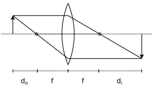
Figure 2.2: Image formation by an ideal thin lens using geometrical optics analysis. Rays parallel to the optical axis of a lens converge at the focal point on the opposite side of the lens. Tracing two rays from a point on an object placed in front of a lens reveals where the image of that object will be formed behind the lens.

Geometrical optics analysis—in which light is modeled as straight, non-diverging rays—provides a framework to discuss the magnification in an imaging system. An

ideal, convex thin lens causes light rays parallel to the optical axis (infinity-focused

light) incident on one side of the lens to converge at a single focal point that lies on

the optical axis on the other side of the lens. The axial distance from the center of the

lens to the focal point is known as the focal distance, f, of the lens. When an object is placed in front of a convex lens, an image of the object is formed behind the lens, as

seen in Figure 2.2. The thin-lens equation relates the axial distance from an object to a lens, do, to the image of the object formed by the lens, di, as

1

f =

1

do

+ 1

di

. (2.2)

The linear magnification provided by the lens is the ratio of the image distance to the

(32)

object distance,

M = di

do

. (2.3)

Microscopes are compound systems of lenses, and the basic principles of their imaging

can be understood with repeated application of the thin-lens equation. In the microscope

diagram of Figure 2.1, the specimen is placed slightly in front of the front focal point of

the objective lens. The magnified intermediate image is formed at the front focal plane

of the tube lens. The total magnification provided by this compound lens system at the

observation image plane is the product of the magnifications from the objective and tube lenses. Under a strict geometrical analysis, then, the image formed of a semitransparent

planar object is

I(x, y) = 1

MLT

x

M, y M

, (2.4)

whereM is the magnification of the system,Lis the uniform illumination intensity, and

T(x, y) describes theoptical transmission of the object—the fraction of light passed by each point in the object.

Most modern microscopes have interchangeable objective lenses of different focal

lengths that offer different magnifications in the microscope system. In aparfocalsystem, the matched objectives for a particular microscope form the intermediate image at the

same location in order to minimize the need to refocus after changing objectives [FHC03].

The distance between the focal points of the objective and tube lenses stays fixed—this

is known as the optical tube length (OTL).

The numerical aperture (NA) of the objective lens measures the light-gathering

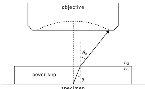
abil-ity of a microscope, which impacts its resolution limit. Letθ2 be the solid half angle of

light admitted into the objective from a point in the center of the specimen plane, as depicted in Figure 2.3. NA is defined as:

(33)

Figure 2.3: The numerical aperture of an objective lens is proportional to the sine of the half-angle of light admitted by the lens. The index of refraction of the medium between the cover slip and objective lens determines the maximum obtainable NA.

where n2 is the index of refraction of the medium between the specimen and objective

lens. The range of this refractive index is n2 ∈ [1.0. . .1.5] with commonly used media

including air (n2 = 1.00), water (n2 = 1.33) and oil (n2 = 1.52) [Mur01].

Observing specimens through a glass cover slip places a constraint on the maximum

obtainable NA. Light rays traveling through the cover slip are refracted at the boundary of the cover slip, as see in Figure 2.3. The angle of incidence and refraction for two

mediums with refractive indices (n1, n2) are related by

n1sinθ1 =n2sinθ2. (2.6)

Total internal reflection occurs when the angle of refractionθ2 ≥ π₂—all light is reflected

into the cover slip. The critical angle of incidence above which total internal reflection

(34)

occurs is therefore

θc1 = arcsin

n2

n1

, (2.7)

which is defined when n1 ≥ n2. From Equations 2.6 and 2.5, the theoretical maximum

NA is equal to the index of refraction of the medium between the cover slip and lens.

For example, air and cover slip glasses have refractive indices ofna = 1.00 andnc = 1.52,

respectively. The critical angle for the cover slip-air interface is therefore θc1 ≈ 41.8◦.

The practical value is slightly less than this, so dry objectives are limited to NAs of

about 0.95. NAs of greater than 1 are obtainable using an immersion medium of water (n2 = 1.33) or oil (n2 = 1.52) between the cover slip and objective lens.

The impact of NA on the microscope resolution limit is discussed in Section 2.1.3,

after a more formal discussion of image formation.

2.1.2 Fourier Optics Analysis

As seen in Equation 2.4, geometrical optics analysis predicts that images formed by

lenses are perfect magnified representations of objects. In fact, diffraction and lens

aberrations cause the image of a point to spread out over a small area in the image

plane. The blurred image of a point on the observed object is defined by the optical

system’s point-spread function (PSF). Even for an object that is in perfect focus, light

rays reflected or transmitted from a point are not all projected to a single point in the image plane.

The image analysis literature provides several models of point spread functions for

optical systems. A geometrical optics approach obtains a PSF by projecting the aperture

of the optical system onto the image plane. Watanabe and Nayar use such an approach

in obtaining shape information by analyzing the defocus of textured surfaces [WN97,

WN98]. The projection of a circular aperture yields a “pillbox” function, where the

(35)

this model does not consider diffraction effects, it is appropriate for macroscale imaging

applications, but not for microscopy.

Cheezum et al. use the following radially symmetric PSF to simulate images of

particles in fluorescence microscopy [CWG01], derived from Born and Wolf [BW75]:

PSF(r) =

2J1(ra)

r

2

(2.8)

a = 2πNA

λ , (2.9)

where r is the radial distance from the center of a point in the geometrical optics projection, λ is the wavelength of light emitted by the fluorescing particle, and J1 is

the first order Bessel function. As shown below, this equation describes the PSF for a

microscope considering diffraction effects but only when the object is in perfect focus.

The work presented here involves both diffraction and focus effects, so a more complete

model of image formation is required.

Fourier optics analysis, which considers the diffraction and interference of light waves,

provides a complete method for understanding how light propagates through space to form images in a microscope. Joseph Goodman’sIntroduction to Fourier Optics provides

a thorough discussion of the image formed by placing a semitransparent planar object

in front of a convex lens [Goo68, Ch. 5 & 6]. A brief overview follows.

Fourier optics analysis is based on the propagation of complex-valued EM radiation

fields through space. Let Uo(xo, yo) be the complex EM field immediately in front of a

semitransparent planar object that has been illuminated by a planar EM wave. When

placed in front of a lens, the field formed at a point in the image plane, Ui(xi, yi), is the

integral of the shifted product of the object field with the PSF, h(xi, yi;xo, yo):

Ui(xi, yi) =

Z Z ∞

−∞

h(xi, yi;xo, yo)Uo(xo, yo)dxodyo. (2.10)

(36)

That is, the PSF provides the optical system output at a location (xi, yi) in the image

plane due to an impulse in the object plane at (xo, yo). Although the PSF in

Equa-tion 2.10 is dependent on both object plane and image plane coordinates, this is purely

a matter of formality at this point—the PSF will be shown to be shift invariant,

depen-dent only on the difference in coordinates, (xi−xo, yi−yo). With a shift-invariant PSF,

Equation 2.10 represents a convolution.

The task remains to determine how the EM field propagates from a point on the

object field through a lens and onto an image plane. The EM field radiates spherically from the point source, and this spherical wave is incident on the lens. The lens aperture

admits a portion of the wave front which diffracts in the region beyond the aperture.

It is the finite aperture, not the lens itself, that gives rise to diffraction in an optical

system—light diffracts after passing through an aperture whether or not a lens is present.

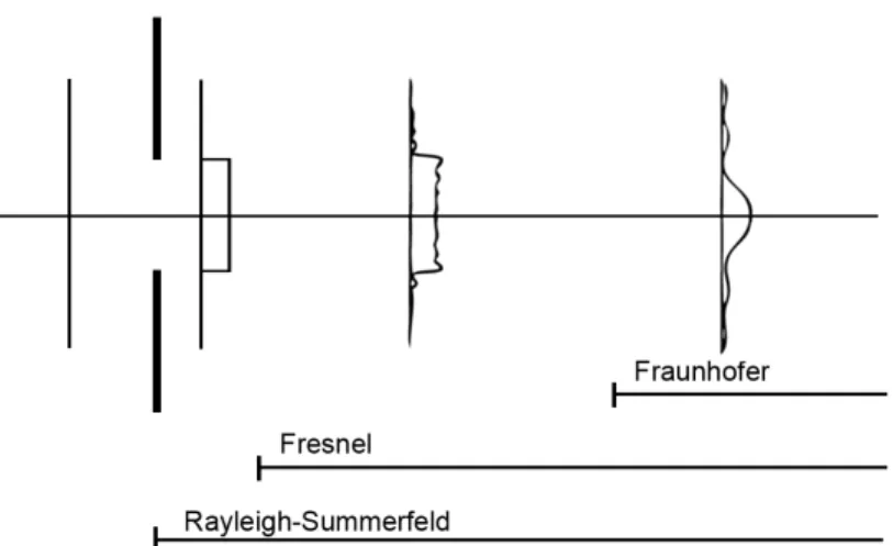
Figure 2.4: The profiles in this figure represent the intensity of a planar wave front propagating from left to right and passing through an aperture. The diffraction of light admitted through an aperture is described by the Rayleigh-Sommerfeld equation at all distances from the aperture. The Fresnel and Fraunhofer equations become valid approximations to the Rayleigh-Sommerfeld equation at distances farther from the aperture [Gas78].

Several equations describe the diffraction of light admitted by an aperture, the most

(37)

distance from the aperture [Gas78, Ch. 10]. As depicted in Figure 2.4, two other

equations are approximations to the Rayleigh-Sommerfeld equation that are valid in

regions some distance away from the aperture. In microscopy, the image plane is very

far from the objective lens aperture where the far-field approximations provided by the

Fraunhofer equations are sufficient. (Note that Figure 2.4 serves only as an illustration

of diffraction regions—it depicts a planar wave incident on an aperture, whereas the

light from a point source incident on an objective lens is spherical. It is the aperture,

not the shape of the wave front nor the presence of the lens, that causes diffraction.) Goodman employs the Fraunhofer diffraction equation and the assumption that the

imaging application is concerned with measuring the light intensity (not phase) of the

image formed—which is the case in microscopy—to arrive at the following approximation

of the PSF:

h(xi, yi;xo, yo)≈

1

λ2_d

odi

Z Z ∞

−∞

P(x, y)e ik 2 1 do + 1 di − 1 f

(x2+y2)

×e

−ik

xo

do

+xi

di x+ yo do

+ yi

di

y

dxdy, (2.11)

whereλ is the monochromatic frequency of light emitted by the point source, do and di

are the axial distances from the lens to the object and image planes, respectively,k = 2_λπ is a wave number, and P(x, y) is the lens aperture function.

For example, the lens aperture function for a circular aperture of radius a is

P(x, y) =       

1 if px2₊_y2 _≤_a

0 otherwise.

(2.12)

Here, the physical lens aperture radius a expressed in terms of NA is

a =dosinθ=

doNA

n , (2.13)

(38)

not dotanθ, as might be assumed from Figure 2.3 [Paw06, Ch. 11].

Returning to Equation 2.11, making the following substitutions

M = di

do

(2.14)

x0_o =−M xo y0o =−M yo (2.15)

yields

h(xi−x0o, yi−yo0) =

1

λ2_d

odi

Z Z ∞

−∞

P(x, y)e iπ λ 1 do + 1 di − 1 f

(x2+y2)

×e

−i2π λdi

[(xi−x0o)x+ (xi−x0o)y]

dxdy. (2.16)

This equation represents a comprehensive, shift-invariant PSF model that considers

both diffraction and defocus effects. That is, evaluating Equation 2.16 for a fixed object distance do provides a slice of the 3D point spread function of the microscope. Note

that the integral is evaluated over the domain of the aperture function while the PSF

is defined over the coordinate differences between the image and object planes (xi −

x0_o, yi−y0o).

When the term 1

do

+ 1

di

− 1

f = 0 in Equation 2.16, the thin lens Equation 2.2 is

satisfied. Under this condition the object is in focus—in fact, this is where the thin

lens equation is derived from. Goodman notes that at optimal focus the PSF is the Fraunhofer diffraction pattern of the lens aperture,

h(xi−x0o, yi−y0o) =

1

λ2_d

odi

Z Z ∞

−∞

P(x, y)e

−i2π λdi

[(xi −x0o)x+ (xi−x0o)y]

dxdy. (2.17)

The Fraunhofer diffraction of a circular aperture is known as theAiry disk, as seen in

(39)

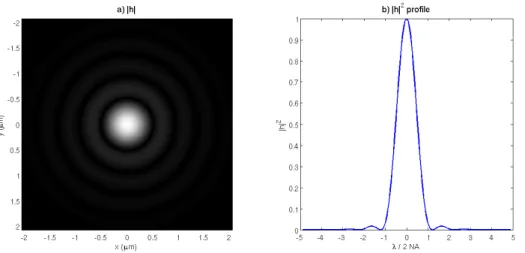
Figure 2.5: A simulated point spread function for a 40X dry objective lens with circular aperture and NA = 0.65. a) The image of the PSF, with size measured in object plane coordinates. b) The profile of the normalized PSF, with units _2NAλ . The first minimum occurs at r= 1_2NA.22λ.

solution gives rise to the PSF model used by Cheezumet al. described by Equation 2.8.

At optimal focus, the image formed by the objective lens most closely resembles

the object placed in front of the lens. The distortion in the image is a result of the lens aperture selecting a fraction of the light diffracted from from the object. Because

light that is diffracted more is excluded, and this diffracted light carries high frequency

information, the lens behaves as a non-ideal low-pass filter. A section of the microscope

PSF through the XZ plane, seen in Figure 2.6, demonstrates how the more general

Equation 2.16 behaves when the object is out of focus.

Microscopy imaging is not concerned with the complex electromagnetic field formed

at the image plane, but rather the intensity of that field. Expressing Equation 2.10 in

terms of image intensity yields

Ii(xi, yi) =

Z Z ∞

−∞

|h(xi−xo0, yi−x0o)|

2

Ig(x0o, y

0

o)dx

0

ody

0

o, (2.18)

(40)

Figure 2.6: The XZ plane of the microscope PSF shows the effect of focus at different distances from the optimal focus plane (z = 0). Low intensity values are emphasized in this image using Io = 4

√

(41)

where Ig(x0o, y

0

o) is the image predicted by geometric optics,

Ig(x0o, y

0

o) =

1

MUo

x0_o M,

y0_o M 2 , (2.19)

which is the complex field form of Equation 2.4. The normalized frequency representa-tion of |h|2 _{is known as the optical transfer function (OTF) of the system}

H(fX, fY) =

F {|h(xi, yi)|2}

RR∞

−∞|h(xi, yi)|2dxidyi

, (2.20)

where F {h} is the Fourier transform of h. Combined with the convolution theo-rem [FvDFH97, Ch. 14], the OTF provides a convenient way to express Equation 2.18

as a product of Fourier transforms

Ii(fX, fY) =H(fX, fY)Ig(fX, fY), (2.21)

where I =F {I}, the Fourier transform of I.

In summary, Fourier optics analysis provides the tools necessary to predict the image

of an object formed in a bright-field microscope. For a semitransparent object, the

process requires finding the PSF of the objective lens for the distance from the object

to the lens. Convolution of the magnified image of the object predicted by geometrical

optics with the PSF yields the image produced by the optical system.

2.1.3 Resolution

Several empirical conventions are used to specify the resolution limit of a light

micro-scope. The Rayleigh criterion specifies the minimum distance between two point sources that can be distinctly identified as

r = 1.22λ

2NA, (2.22)

(42)

whereλis the wavelength of light used for the observation. This criterion follows directly from Equation 2.17, the focused PSF. As shown in Figure 2.5, at this distance, the peak

at the center of one point’s Airy disk coincides with the first minimum of the other

point’s Airy disk. For example a microscope equipped with an oil immersion objective

lens with NA = 1.4 using monochromatic illumination with green light (λ = 550 nm) has a theoretical minimum resolvable distance between two points of

r = 1.22∗550 nm

2∗1.4 ≈240 nm. (2.23)

The Abbe limit is another convention that pertains to the ability to resolve repeating

patterns in a specimen, such as a diffraction grating or muscle striations. Light waves

admitted through neighboring gaps in the specimen diffracts and interferes, leading to interference patterns in the resulting wave front. In order to resolve a repeating

structure, the undiffracted and 1st _{order interference patterns must be collected by the}

objective lens. The distance between the orders of interference patterns depends on the

pattern spacing; the smallest pattern that can be resolved is

d= λ

2NA. (2.24)

Though the constant terms in Equations 2.22 and 2.24 are different, under either

criterion the resolution limit is defined by the wavelength of light and the objective NA.

Bounds on the resolution limit of a light microscope are placed by the wavelength of

ob-servable (visible or otherwise detectable) light and the index of refraction of practically

useful immersion media. For visible light microscopy, one cannot improve significantly on the values used in Equation 2.23. Electron microscopy leverages the shorter

wave-length behavior of electrons to examine specimens at a higher resolution. Structured

illumination techniques, such as those discussed in Chapter 3, use multiple images with

(43)

fluores-cence microscopy.

The NA also determines the depth of field in a microscope image. The sharpest

image is formed of objects in the focal plane; image sharpness decreases as objects move

away from the focal plane. Objects within a small distance of the focal plane can still

be said to be in focus if their image is reasonably sharp. Smaller depths of field are

desirable for fine optical sectioning of a specimen. With larger depths of field, more of

the specimen contributes to the image, though not all components are equally focused.

Like the resolution limit, defining the depth of field is, to a large degree, a matter of convention—for an image sensor with a minimum resolvable distance ofe, one empirical convention specifies the depth of field as

d= λn NA2 +

ne

MNA. (2.25)

Intuitively, the angle of the cone of light admitted into the objective lens (as determined

by the NA) corresponds to a cone of light that is focused on the image plane for each

point on the object. As the object moves further from focus, a wider disk is projected

onto the image plane. As higher NAs admit broader cones of light, this disk size is

larger at a fixed distance from focus for higher NAs. The second term in Equation 2.25

depends on the resolvable distance of the sensor, e. For a regular grid array—as used in digital image acquisition, described next—this is empirically set to be the distance

spanned by three sensor elements. Two objects can be distinguished if they illuminate

two sensor elements with an non-illuminated element between them.

2.2 Image Acquisition

Section 2.1 discussed how bright-field microscopes form images; this section discusses

how these images are digitized for computer storage and analysis. Fourier optics explains

that the image formed by a microscope is a complex EM field. When projected onto a

(44)

surface and observed, a microscope image is a continuous function of irradiance—the

power of light energy incident on a surface area [FP03, Ch. 4]. A charge-coupled device

(CCD) image sensor is commonly used in image acquisition to sample the continuous

distribution of light to produce a digital image.

A digital image is a collection of data organized in a structured, regular grid, for

example a two-dimensional array of intensity values [FvDFH97, Ch. 14 & 17]. A digital

image is composed of picture elements—pixels—each of which has a coordinate position

and data value defined at that coordinate location. A digital image is therefore a discrete function over the domain of grid locations.

In the convention adapted for this work, pixel coordinates specify the center of a

pixel and the pixel value is strictly defined only at the center of pixels. This work is

concerned with the analysis of time sequences of two-dimensional (2D) images. Other

types of images may be generated through this analysis, for example 2D vector images

that describe motion fields.

2.2.1 Charge-Coupled Devices

The image formed by a CCD is a sampled representation of a continuous distribution

of light. A CCD is composed of a regular grid of photosensitive elements that operate under the principles of the photoelectric effect. When light is incident on a metal,

photons may interact with electrons in the metal. A photon can transfer its energy to

an electron, possibly ejecting the electron from the atom to which it is bound. A freed

photoelectron can be trapped in a potential energy well associated with a photosensor

site on a CCD.

A CCD captures freed photoelectrons over the exposure time period [HK94]. At the

end of the exposure, the electrons in each potential well are transfered sequentially to

(45)

stream by an analog-to-digital converter (ADC). This stream of digital pixel values is

transferred from the camera to a storage device or computer for storage and analysis.

If the purpose of a CCD is to measure photoelectrons created by a distribution of light

intensity on a surface, the ideal value, I(x, y), recorded by a camera for an individual sensor element would be proportional to the number of photons incident on the sensor

integrated over the exposure period, E(x, y):

I(x, y) =kE(x, y), (2.26)

where k is the device-specific constant of proportionality. Of course, it is impossible to accurately measure the incident intensity function E(x, y) exactly—several types of noise corrupt the image acquisition process [HK94, TRK01, FP03]. Understanding the character of these noise sources is important for accurate image analysis and simulation

tasks, such as those described in this dissertation. Below I construct the CCD imaging

model used by Healey and Kondepudy while explaining each source of noise.

The arrival of photons at a sensor site is a Poisson-distributed random process [HK94]

that leads to the random effect known asshot noise. The photoelectron count at a site

is therefore a sample of a Poisson random variable, Ns with variance equal to the ideal

number of photoelectrons collected:

I(x, y) =Ns(kE(x, y)). (2.27)

Healey and Kondepudy represent shot noise with a Poisson distribution that is shifted

to have zero mean, implicitly making the following manipulation:

I(x, y) = kE(x, y) + (Ns(kE(x, y))−kE(x, y)) (2.28)

= kE(x, y) +N_s0. (2.29)

(46)

Shifting the shot noise to have zero mean affords a convenience to the analysis that

follows: when all noise sources are zero-mean and additive, the expected value of a

pixel’s intensity can be obtained by averaging many observations. For this reason, I

adopt this notation here.

Fixed pattern noise arises from different physical sensors having slightly different

sizes and quantum efficiencies, therefore counting a different number of photons for the

same incident light intensity. The fixed pattern noise can be incorporated by the scaling

factorkin Equation 2.26;k(x, y) has a normal distribution with a mean of 1 and variance

σ2

k:

I(x, y) =k(x, y)E(x, y) +N_s0(x, y). (2.30) Thermal energy in the image sensor can also free electrons that become trapped

in the potential energy wells associated with a CCD sensor element. These dark

cur-rent electrons are indistinguishable from photoelectrons and so contribute an additional

source of noise in the image measurement:

I(x, y) =k(x, y)E(x, y) +N_s0(x, y) +Nt(x, y). (2.31)

The dark current increases with exposure time and sensor temperature.

The circuitry that reads out the potentials stored at each sensor site contributes a

small, zero-mean, Gaussian-distributed noise, modeled by Nr:

I(x, y) = k(x, y)E(x, y) +N_s0(x, y) +Nt(x, y) +Nr(x, y). (2.32)

Equation 2.32 represents the number of electrons collected as the input signal to the

(47)

the ADC involves an additional noise term,Nq:

I(x, y) = (k(x, y)E(x, y) +N_s0(x, y) +Nt(x, y) +Nr(x, y))A+Nq(x, y). (2.33)

Healey and Kondepudy argue that Nq is approximately zero-mean and uniformly

dis-tributed over [−q

2,

q

2], where q is the quantization step size. This equation represents

the actual imageI(x, y) recorded by a CCD in response to an ideal photoelectron count function E(x, y). Rearranging a few terms yields a convenient form:

I(x, y) = µ(x, y) +N(x, y), (2.34)

µ(x, y) = k(x, y)E(x, y)A+µt(x, y)A,

N(x, y) = N_s0(x, y)A+Nr(x, y)A+Nq(x, y).

Here, µ(x, y) is the expected value of I(x, y), µt(x, y) is the expected value of the dark

current, Nt(x, y), which is the only non-zero-mean noise source, and N(x, y) is a

zero-mean random variable that encapsulates all other temporal noise sources.

In summary, the formation of digital bright-field microscopy images consists of the following key components:

1. K¨ohler illumination ensures that a uniform light field illuminates the specimen.

2. The microscope’s objective gathers light transmitted through the specimen,

form-ing an image of the specimen convolved with the microscope’s PSF on the image

sensor.

3. The image sensor integrates the light irradiance distribution function over an ex-posure time by counting photoelectrons collected in a regular grid of potential

energy wells.

4. The camera scans the charges collected at each sensor site and digitizes these

(48)

sensor values.

5. A computer saves the collected digital image for further image processing.

2.3 Camera Calibration

Working with the CCD image acquisition model of Equation 2.33, it is possible to

characterize and calibrate the image sensor in a camera attached to a bright-field

mi-croscope. I close this chapter with a practical camera calibration procedure, based on

the combined wisdom provided by several camera calibration procedures [HK94, TV98,

TRK01, MMG05]. To illustrate the procedure, I present calibration results obtained

from a Pulnix TM-6710CL progressive scan, monochrome, 8-bit camera, which records

648×484 pixel2 images at a maximum rate of 120 fps. The camera is attached to an inverted Nikon Eclipse TE2000-E microscope with an optical train modified to

accom-modate other optical components such that strict K¨ohler illumination is not possible:

the microscope is missing a collector lens and aperture diaphragm.

2.3.1 Dark Current Estimation

The thermal noise in an acquired image introduces a positive offset at each pixel. Taking

a series of dark images enables estimating the expected value of this offset. A series of

dark images is obtained by turning off the microscope lamp and covering the camera

aperture to block all light from the image sensor. If the camera aperture cannot be

blocked, the room lights can be turned off to make the acquisition environment as dark as possible. A series of nd images are then acquired using the exposure settings that

will be used in future image acquisition.

From the model of Equation 2.34, each dark image is

(49)

and the mean of nd dark images has expected value µt(x, y)A and variance

σ_N2 nd

:

ˆ

Id(x, y) =

1

nd nd X

i=1

Idi(x, y) = µt(x, y)A. (2.36)

The mean dark image, ˆId(x, y), can be subtracted from any image taken with the same

exposure settings to obtain a dark-current-corrected image. For the Pulnix camera operating at 120 fps, ˆId(x, y) has a mean value of 3.252 × 10−6 counts and a mean

variance, σ2

N = 3.267 ×10

−6 _counts2_{. The dark current offset for this camera can}

therefore reasonably be neglected.

2.3.2 Flat-field and Fixed-pattern Noise Estimation

Despite the best efforts to align the optical elements in a microscope, the illumination

field provided even by K¨ohler alignment is never truly uniform. Each sensor in the

CCD receives a different intensity of light, so the effect of nonuniform illumination is a

per-pixel scaling of the photoelectron count. In the CCD model of Equation 2.33, the

parameter k(x, y) can therefore incorporate both fixed-pattern noise and nonuniform illumination effects. Accounting for nonuniform illumination is known as flat-field

cor-rection. To calibrate a flat-field image, the microscope is adjusted for uniform K¨ohler

illumination, and a clean, blank slide and cover slip are placed on the stage. A series

of nf images of this approximately uniform field is acquired at a single lamp intensity.

The mean of these images, ˆIf(x, y), has the expected value

ˆ

If(x, y) = k(x, y)E(x, y)A+µt(x, y)A. (2.37)

(50)

The termµt(x, y)Ais estimated by dark current calibration as described in Section 2.3.1,

and can be subtracted to provide

ˆ

If(x, y)−Iˆd(x, y) =k(x, y)E(x, y)A. (2.38)

Because k(x, y) has expected value 1, the mean value of this resulting image is an estimate of EA, the signal that an ideal sensor would register everywhere for a uniform illumination. Thus,

µf =

1

nm

n

X

x=1

m

X

y=1

ˆ

If −Iˆd=EA, (2.39)

F(x, y) = ˆ

If(x, y)−Iˆd(x, y)

µf

= k(x, y)E(x, y)A

µf

=k(x, y).

Figure 2.7: A flat-field calibration image obtained from the Zeiss microscope and Pulnix camera.

(51)

field images captured at 120 fps. The flat-field image values fall within the range

[0.574. . .1.288] with variance 6.84×10−3_{. This image reveals that the lamp is not}

prop-erly aligned with the center of the camera. The diagonal banding lines are fixed-pattern

aberrations probably arising from electrical interference from some other component in

the microscope system. The dark splotches in the image are from dust on the image

sensor or dirt on the slide. There are several columns on the left side of the image where

the signal drops considerably; this indicates that the image sensor may not be properly

seated in the camera enclosure.

The calibration images F(x, y) and ˆId(x, y) provide a means to correct any image,

I(x, y), taken under the same conditions as the calibration images, including frame rate, lamp level, optical alignment, and slide and cover slip thickness. From Equations 2.33,

2.36, and 2.39, a corrected image is

Ic(x, y) =

I(x, y)−Iˆd(x, y)

F(x, y) (2.40)

= E(x, y)A+Ns(x, y)A+Nr(x, y)A+Nq(x, y).

2.3.3 ADC Gain Estimation

The gain applied by the ADC can be approximated using a number of images of a

uniform field taken at different illuminations. The variation in uniform field images

(or small regions of interest) should be due to the noise introduced by the CCD image

acquisition and not from illumination inconsistencies. It is not necessary to use flat-field

corrected images for this process provided that a reasonably uniform region can be found

within the calibration images.

To obtain calibration images for gain estimation, the microscope is adjusted for

uniform K¨ohler illumination, and a clean, blank slide and cover slip are placed on the stage. The lamp intensity is set to a high level that does not cause clipping (clamping

to the maximum intensity output by the camera) of the acquired images. Pairs of

(52)

images are then captured at different illumination levels, ideally by inserting several

neutral density filters into the optical train. Alternatively, a large number of images

are acquired while the lamp is slowly dimmed, and any consecutively captured pair of

images is considered to be obtained at the same intensity setting. This approach is

not as robust as using neutral density filters because dimming the lamp changes the

spectrum of light emitted, and the CCD sensor response depends on the frequency of

incident light.

Given a pair of images I1(x, y) and I2(x, y) captured at the same intensity, the

summed image, IΣ12(x, y) = I1(x, y) +I2(x, y), has expected value

µΣ12 =

1

nm

n

X

x=1

m

X

y=1

IΣ12(x, y) (2.41)

= 2µ(x, y) = 2(k(x, y)E(x, y)A+µt(x, y)A),

where each image has dimensions n×m. The difference image, I∆12(x, y) = I1(x, y)−

I2(x, y), has variance

var[I∆12] = 2σ2N. (2.42)

At a high intensity level, Healey and Kondepudy show that

σ_N2 =Aµ+σ_c2, (2.43)

where σ2

c is the variance of NrA +Nq, the temporal noise that does not depend on

the electron count. Given ni pairs of images taken at multiple intensity levels, linear

least-squares regression can be used to find maximum likelihood estimates for the gain,

A and constant noise variance, σ2

c.

Figure 2.8 shows the results of gain calibration on the Pulnix camera capturing

images at 120 fps. Images are obtained using the lamp dimming approach because the

(53)

Figure 2.8: Gain calibration for a CCD image sensor involves acquiring a series of paired images at multiple intensity settings. a) A selection uniformly illuminated image patches obtained by slowly dimming the lamp while capturing images at 120 fps. b) The gain calibration obtained by plotting σ2

N vs. µfor all consecutive

image pairs. The dashed line shows the fit of Equation 2.43 computed with linear least-squares regression.

(54)

the Pulnix, this approach produces calibration estimates based on a large number of

samples, 2399 image pairs in this case. The mean value and variance of the sum and

difference images are computed from a 100×100 pixel2 region of interest that is selected for having approximately uniform illumination and no fixed aberrations (e.g. dirt on the

image sensor or slide). Linear regression reveals a sensor gain of A= 7.56×10−3 _counts

per electron (130 electrons / count) and a constant noise variance ofσ2_c = 0.289 counts2. This gain estimate provides a basis for the noise model used in simulating microscopy

(55)

Chapter 3 Related Work

This work is concerned with forming models of motion and structure in multiple layer

imaging scenarios. Biological microscopy provides numerous examples of multiple layer

imaging. Biological specimens are usually semitransparent, and the microscope optics

impose a non-zero depth of field. For this reason, the images formed in a microscope

are a composition of multiple scene elements.

The unconstrained motion problem—determining the motions that explain intensity differences between images—is ill-posed, as any mapping that assigns all pixels in one

frame with a particular intensity to a single pixel in the next frame with the same

intensity is “valid.” All motion analysis research is therefore based on some set of

assumptions about the imaging system and the observed scenes. The computation

of motion for rigid and deformable opaque objects is well studied. The scenarios for

which computing multiple layer motion has been solved remains more limited. The

human visual system, however, is able to comprehend multiple layer motions in many

more situations—although it is prone to optical illusions caused by balanced opposing motion signals [QAA94]. The human visual system provides a proof by example that