STATISTICAL METHODS FOR EVALUATING
THE DIAGNOSTIC ACCURACY OF
INCOMPLETE MULTIPLE TESTS
Yi Zhang
A dissertation submitted to the faculty of the University of North Carolina at Chapel Hill in partial fulfillment of the requirements for the degree of Doctor of Philosophy in the Department of Biostatistics.
Chapel Hill 2013
Approved by:
c
2013 Yi Zhang
Abstract
YI ZHANG: STATISTICAL METHODS FOR EVALUATING THE DIAGNOSTIC ACCURACY OF INCOMPLETE MULTIPLE TESTS
(Under the direction of Donglin Zeng and Haitao Chu)
Acknowledgments
Table of Contents
List of Tables . . . viii
List of Figures . . . ix
1 Introduction and Literature Review . . . 1
1.1 Diagnostic Accuracy for Binary Tests . . . 1
1.2 Diagnostic Accuracy Evaluation without a Gold Standard . . . 2
1.2.1 Discrepant Analysis . . . 2
1.2.2 Composite Reference Standard . . . 3
1.2.3 Expert Review Panel . . . 4
1.2.4 Latent Class Analysis (LCA) . . . 4
1.3 Evaluation with a Partially-Missing Gold Standard . . . 7
1.3.1 Case-Deletion Approach . . . 8
1.3.2 Correction Methods . . . 8
1.3.3 Imputation Methods . . . 9
1.3.4 Expectation-maximization Algorithm . . . 10
1.4 Outline for the Dissertation . . . 10
2 Conditional Independence Assumption . . . 12
2.1 Introduction . . . 12
2.3 Statistical Methods . . . 16
2.3.1 Diagnostic Performance under a MAR Assumption . . . 17
2.3.2 An Extension to One MNAR Scenario . . . 18
2.3.3 Model checking using Kappa statistics . . . 19
2.4 Analysis of the Colon Cancer Family Registry . . . 20
2.5 Simulation Studies . . . 21
2.6 Discussion . . . 25
3 Conditional Dependence Assumption . . . 32
3.1 Introduction . . . 32
3.2 Motivating Example . . . 35
3.3 Statistical Methods . . . 37
3.3.1 PLC Model Parameters Specification and Expansion . . . 37
3.3.2 ML Estimation Using the Monte Carlo EM Algorithm . . . 39
3.3.3 Starting Values for the PX-MCEM Algorithm . . . 45
3.3.4 Bootstrap Method for Standard Errors . . . 47
3.4 Simulation Studies . . . 48
3.5 Results . . . 53
3.6 Discussion . . . 54
4 DiagLCA - An R Package for the Evaluation of Binary Tests . . . . 68
4.1 Introduction . . . 68
4.2 Methodology . . . 71
4.3 The R Package DiagLCA . . . 75
4.3.1 FunctionindTLC . . . 75
4.3.2 FunctiondepPLC . . . 76
4.3.4 Functiontraceplot . . . 79
4.3.5 Functionconvergplot . . . 79
4.3.6 Functionhistgram . . . 79
4.3.7 Functionqqplot . . . 80
4.3.8 Functionsimudata . . . 80
4.4 Implementation . . . 82
4.4.1 Example Data . . . 82
4.4.2 Initial Exploration . . . 82
4.4.3 Fitting a TLC Model . . . 84
4.4.4 Fitting a PLC Model . . . 86
4.4.5 Simulate Data Sets for Simulation Studies . . . 92
4.5 Summary . . . 95
5 Future Research . . . 101
Appendix : Derivation of Information Matrices for Louis Formula . . 104
List of Tables
2.1 Summary of EM Estimates and Coverage of 95% CIs for Simulated Data under Different Missing Pattern Assumptions . . . 23
2.2 Number of Subjects by Frequency of Missing Test Results . . . 29
2.3 Estimates and 95% CIs of Sensitivity, Specificity, and Prevalence from Different Models . . . 30
2.4 Estimates and 95% CIs of r1j, r0j, and rj under Different Missing Data Assumptions . . . 31
3.1 Summary of Simulation Results . . . 52
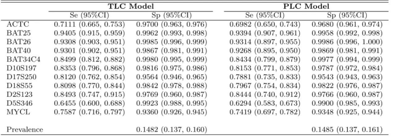
3.2 Estimates and 95% CIs of Se, Sp, and Prevalence from Different Models 66
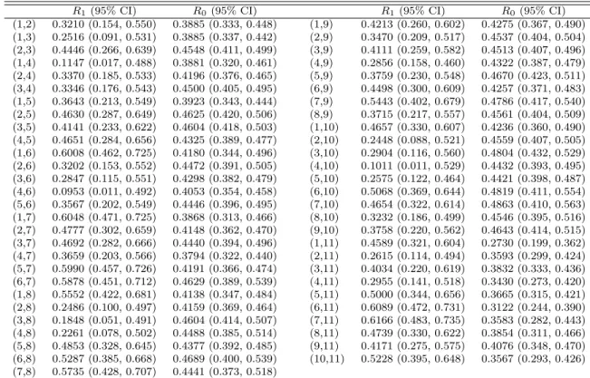
3.3 Estimates and 95% CIs of R1 and R0 from the PLC Model . . . 67
List of Figures
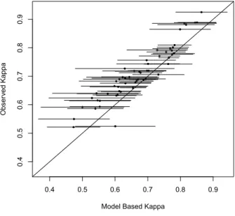
2.1 Plot of Observed vs. Model Based Kappa . . . 28
3.1 Correlation Residual Plots for C-CFR Data . . . 59
3.2 Correlation Residual Plots for Simulated Data Sets . . . 61
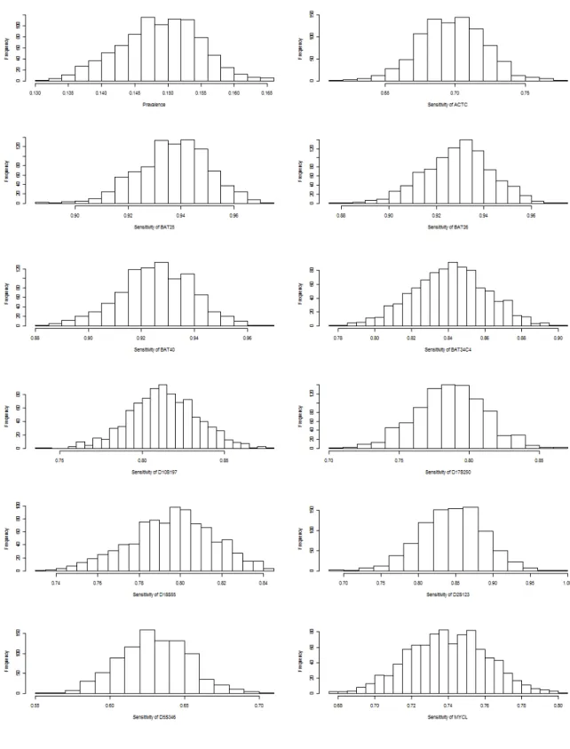
3.3 Histograms of Bootstrap Samples (B=1000) for Prevalence and Diagnos-tic Accuracy . . . 62
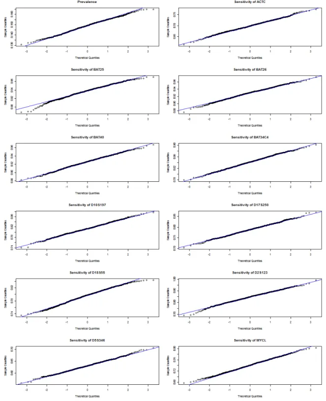
3.4 QQ Plots of Bootstrap Samples (B=1000) for Prevalence and Diagnostic Accuracy . . . 64
4.1 Observed vs. Model Based Kappa for Model Checking . . . 97
4.2 Trace Plot of PKk=1nkd
(m)
k z
(m)
k1 over the Last PX-MCEM Algorithm
It-eration . . . 98
4.3 Convergence Plot of Sensitivity Estimates . . . 99
Chapter 1
Introduction and Literature Review
1.1
Diagnostic Accuracy for Binary Tests
Accurate diagnosis of a disease or classification of a subtype of a disease is often the first step toward the treatment and prevention of the disease. A diagnostic test is expected to contribute to a reliable diagnosis of a patient’s medical condition and aid in the health practitioner’s development of an appropriate treatment plan. Misdiagnoses are likely to result in mislead health practitioners’ initiating unnecessary or incorrect treatment plans. Therefore, evaluation the diagnostic accuracy of a test is pivotal to medical practices.
are often referred to as false positive and false negative error rates associated with a test. Neither sensitivity nor specificity is affected by the prevalence of the disease. This crucial property makes estimates of sensitivity and specificity from one study readily applicable to other studies in which the prevalence of the disease was different. Nevertheless, sensitivity and specificity may be affected by the stages of the disease or by patients’ characteristics (e.g., different densities of fat tissue). Ledley and Lusted (1959) made some early contributions to the paradigm of diagnostic accuracy.
Ideally, the sensitivity and specificity of a new test are evaluated by comparing its results with the true status/condition of the disease (presence or absence) in a subject, which is the result of a test with a perfect ability to classify the disease; such a test is referred to as a ‘gold standard’. In other words, a gold standard is an error-free reference standard with a sensitivity of 100% and a specificity of 100%. In practice however, a gold standard is often impossible to find, or it simply may not exist. Multiple imperfect diagnostic tests often are used in the absence of a gold standard. These tests are either applied simultaneously to one subject and interpreted altogether or applied sequentially in a prespecified order. The latter is usually more cost-effective but less efficient, since the decisions of whether to administer subsequent tests and when to administer them depend on the results of tests that already have been conducted. The next section introduces the common methods that are used to evaluate diagnostic accuracy in the absence of a gold standard.
1.2
Diagnostic Accuracy Evaluation without a Gold Standard
1.2.1
Discrepant Analysis
disease status. When two tests show discrepant results, a resolver test (often with better diagnostic accuracy but which is costly and/or invasive) is chosen to reconcile the discrepancy. This approach is subject to the error rate of the test used to reconcile the discrepancy as well as the error rates in the wrongfully concordant results of the initial tests. The resolver test is assumed to be independent of the preceding tests, which may not be the case. Hadgu (1996, 1997, 1999) posited that discrepant analysis cause serious bias in the estimates of diagnostic accuracy that are obtained and that such estimates are scientifically flawed.
1.2.2
Composite Reference Standard
1.2.3
Expert Review Panel
When no reference standard is generally accepted, an expert review panel may reach a consensus diagnosis concerning the status of a subject with respect to a specific disease using assorted information from different sources, including symptoms/signs, physical characteristics, medical history, clinical follow-ups, and imperfect reference tests. Test results that are undergoing evaluation usually are not presented to the panel for review in order to avoid the incorporation of bias that could lead to an overestimation of the accuracy of the diagnosis. Thornbury et al. (1993) demonstrated a gold standard panel of neurosurgeons, neurologists, and physicians experienced in technology assessment for diagnosis of patients receiving MRI and CT for acute low-back pain. They eliminated bias by using a diagnosis that was independent of the diagnostic test being evaluated. Another practice is to present the results of the diagnostic test that is being evaluated to the panel after they make a decision about the diagnosis, and then determine whether these results would change their opinion. The Delphi method is a formal procedure that collects and integrates the opinions of each individual panel member in an anonymous way to avoid influence among fellow members or from a dominating member (Jones and Hunter, 1995).
1.2.4
Latent Class Analysis (LCA)
in this case is the unobservable, true status of the disease, whereas the manifest vari-ables are the test results.
Estimates of the parameters of diagnostic accuracy can be derived with maximum likelihood (ML) based methods involving iterative computation, such as expectation-maximization (EM) algorithms (Dempster et al., 1977), Fisher scoring (Espeland and Handelman, 1989), and the Newton-Raphson method (Qu and Hadgu, 1998). ML ap-proaches provide a unified framework for various latent class models (LCMs), including the Hui-Walter reference-free method (Hui and Walter, 1980), a Gaussian random ef-fects model (Qu et al., 1996), a marginal model (Yang and Becker, 1997), a joint model approach (Albert, 2009), a finite mixture model (Albert et al., 2004), a model that incorporates multiple latent variables and covariates (Huang and Bandeen-Roche, 2004), a probit latent class (PLC) model with a general correlation structure (Xu and Craig, 2009), and a Bayesian model using the Gibbs sampler algorithm to approximate marginal posterior densities of all parameters (Joseph et al., 1995). In the absence of a gold standard, LCMs have been well reviewed (Walter and Irwig, 1988; Goetghebeur et al., 2000).
age and gender), and similar training/experience of those who rate the test. The earli-est work on LCA relied on the conditional independence assumption (Hui and Walter, 1980; Walter and Irwig, 1988; Rindskopf and Rindskopf, 2006). Torrance-Rynard and Walter (1998) found that LCA under the conditional independence assumption often handled conditional correlated tests well and produced relatively unbiased estimates of diagnostic accuracy. However, for diseases with very low prevalence or for tests with very low specificity, the estimates could be seriously biased with slightly correlated tests. Many studies have shown that ignoring the correlation of misspecification errors between tests led to biased estimates of diagnostic accuracy when the conditional in-dependence assumption does not hold (Thibodeau, 1981; Vacek, 1985; Hui and Zhou, 1998). Most of the recently developed LCA methods relax the conditional indepen-dence assumption (Joseph et al., 1995; Qu et al., 1996; Yang and Becker, 1997; Xu and Craig, 2009; Albert, 2009). Albert and Dodd (2004) showed that estimates of diagnos-tic accuracy and prevalence are sensitive to the choice of dependence structure. The correct dependence structure between tests often is hard to specify, and estimates of the parameters can be biased if the structure is misspecified. To better distinguish the dependence structures between different latent classes, they strongly recommended a large number of tests (ideally 10 or more).
get around intrinsic non-identifiability is to add a plausible restriction to the model, e.g., setting equal sensitivities and specificities for the two tests. Bayesian methods are particularly useful for ill-defined models. The unknown parameters are treated as ran-dom variables with a prior distribution that incorporates pertinent information, such as estimates from similar studies, expert’s opinions about the characteristics of the test, and demographic data about patients or the study population. The prior distribution is updated with new information from observed data to derive the posterior distribution for each parameter. Then, point estimates along with the highest posterior density (HPD) credible sets for diagnostic accuracy are obtained from the posterior distribu-tion. The disadvantages of the ML approaches are that Bayesian approaches usually are intensive computationally, and they are sensitive to the prior distribution that is chosen.
Despite the popularity of LCA, it has been cautioned that estimates of diagnostic accuracy are subject to bias if the underlying assumptions of the model cannot be justified (Albert and Dodd, 2004; Pepe and Janes, 2007; Bertrand et al., 2005). Another concern with LCA is that the true disease status is defined mathematically rather than clinically, which results in scientific doubt among some clinicians about the meaning of the resulting estimates (Pepe, 2004).
1.3
Evaluation with a Partially-Missing Gold Standard
(often less expensive/invasive) is feasible rather than the gold standard. This section covers the evaluation of diagnostic accuracy when only a subset of subjects receives the gold standard.
1.3.1
Case-Deletion Approach
The case-deletion approach excludes all subjects from analysis who were not tested with a gold standard. This method could drastically reduce the power and cause partial verification bias. Sensitivity tends to be overestimated, and specificity tends to be underestimated. The direction and magnitude of the biases are affected by multiple factors, such as the proportion of missing tests, the extent to which the true disease status is dependent on or independent of the missing tests, and the unobserved ratio of positive results to negative results for the missing tests. The case-deletion approach should be avoided unless the missing proportion is very small.
1.3.2
Correction Methods
classification errors between tests was misspecified and found that the bias of adjusted estimates could be worse than the bias of unadjusted estimates.
1.3.3
Imputation Methods
1.3.4
Expectation-maximization Algorithm
The EM algorithm, formalized by Dempster et al. (1977), has been used in many fields, including diagnostic medicine. The DLR paper stimulated great interest in the use of finite mixture distributions for modeling heterogeneous data. Finite mixture or unobserved heterogeneity models are one type of LCM that assumes that the observa-tions of one sample arise from a mixture of two or more unobserved classes of unknown proportions (Day, 1969). Determining ML estimates (MLEs) of mixture models with incomplete data is simplified substantially by the EM algorithm. McLachlan and Peel (2000) reviewed the application of finite mixture models. Dawid and Skene (1979) first used the EM algorithm to determine MLEs of observed error rates when a gold standard was not available, and they regarded the latent disease status as a missing value.
The EM algorithm has an inherent advantage over other methods in that it takes into consideration missing gold standards as well as missing imperfect diagnostic tests. To our knowledge, there is very little literature on evaluating multiple imperfect diagnostic tests with missing data and without a gold standard. For our case study, only a small proportion (6.3%) of the 3,487 subjects has been tested with all 11 biomarker tests. The latent true disease status (due to the absence of a gold standard), along with very high proportions of missing tests, have posed statistical challenges related to the evaluation of their diagnostic accuracy and motivated our research utilizing EM algorithm-based approaches, which will be discussed fully in later chapters.
1.4
Outline for the Dissertation
Chapter 2
Conditional Independence
Assumption
2.1
Introduction
algorithm (Dempster et al., 1977; Dawid and Skene, 1979), Fisher scoring (Espeland and Handelman, 1989), and Newton-Raphson method (Qu and Hadgu, 1998). The ML approaches provide a unified framework for various latent class models (LCMs) in a dispersed literature (Chu et al., 2009; Hui and Walter, 1980; Qu et al., 1996; Yang and Becker, 1997; Albert et al., 2004; Albert, 2009; Huang and Bandeen-Roche, 2004; Xu and Craig, 2009). Walter and Irwig (1988) and Goetghebeur et al. (2000) reviewed LCMs based on ML approaches.
always known), Poleto et al. (2011) proposed a two-stage hybrid procedure (ML in the first stage; weighted least squares in the second stage) in estimating the diagnos-tic accuracy of three index tests with abundant missing data under the MCAR/MAR assumptions.
The aforementioned literature deals with two scenarios: (i) a gold standard does not exist whereas the index tests / imperfect reference standards have no missing value; (ii) a gold standard is available (partially or fully observed). To the best of our knowledge, when a gold standard does not exist, there are no studies on handling missing test results from multiple imperfect diagnostic tests to facilitate the estimation of their diagnostic accuracy. For the Colon Cancer Family Registry (C-CFR) study that we will consider (see Section 2), only a small proportion (6.3%) of the 3,487 subjects has been tested for all 11 biomarkers. The latent true disease status along with very high proportions of missing test results have created statistical challenges for evaluating the population prevalence and the estimates of diagnostic accuracy for the 11 biomarkers. Motivated by the C-CFR case study, we develop a LCM to handle the general case where some subjects may only be tested by a subset of markers. It accounts for missing data under the MAR or MNAR assumptions and unobservable latent disease status simultaneously. Specifically, it allows for differential missing probability of each test to depend on latent disease status under one MNAR scenario. The C-CFR study is described in Section 2. Section 3 introduces the statistical methods. Full analysis of the case study (Section 4) and simulation studies (Section 5) are summarized next. Section 6 presents a brief discussion.
2.2
Colon Cancer Family Registry Study
statistics from NCI and WHO websites). In the United States, about 15,000 new cases of colorectal cancer are diagnosed each year (Ford and Whittemore, 2006). About two to five percent of all colon cancer cases are attributed to hereditary nonpolyposis colorectal cancer (HNPCC), also called Lynch Syndrome after Dr. Henry Lynch. HNPCC is a hereditary syndrome that is caused by a mutation in genes involved in the DNA mismatch repair pathway. People with HNPCC have a much higher risk of developing colon cancer than the general population if they do not undergo early and regular screening. The average age of diagnosis of cancer in patients with HNPCC is 44 years, as compared to 64 years in people without the syndrome (Lynch and de la Chapelle, 1999; DeFrancisco and Grady, 2003).
Microsatellites are common and normal repeated sequences of DNA. Although the length of microsatellites is highly variable from person to person, each individual has microsatellites of set length. In cells with mutations in DNA repair genes, however, some of these sequences accumulate errors and become longer or shorter. The appear-ance of such long or short microsatellites in an individual’s DNA is referred to as mi-crosatellite instability (MSI). MSI is a key factor in several cancers including colorectal, endometrial, ovarian and gastric cancers. Cancers with MSI account for approximately 15% of all colorectal cancers and for HNPCC germline mutations (Boland et al., 1998; Umar et al., 2004; Lynch and de la Chapelle, 1999). The diagnosis of HNPCC may be determined if the cancer exhibits a high level of MSI. People with HNPCC have a much higher risk of developing colon cancer than the general population if they do not undergo early and regular screening.
data includes diagnostic test results of eleven molecular biomarkers (BAT25, BAT26,
BAT40,BAT34C4,D10S197,D17S250,D18S55,D2S123,D5S346,ACTC andMYCL) which are used to assess the level of MSI.
In this paper, we consider the 3,487 subjects from families with a single subject per family. The observed missing proportions range from 7.26% for biomarker BAT26 to 81.73% for biomarker D2S123. Table 2.2 summarizes the number of subjects by frequency of missing test results for the 11 biomarkers. Most of the subjects (93.72%) have at least one test result missing. Specifically, the “missing” category includes the following categories defined by the Colon CFR code book: a) quantity of DNA or tissue not sufficient (code 13); b) not tested, reason not specified (code 12); c) no amplification (code 11); d) equivocal (inconclusive, code 6); and e) normal DNA not used in test (code 9). The high proportions of missing and latent disease status have motivated our methodology research which we introduce in the next section.
2.3
Statistical Methods
The total number of subjects is N = 3,487 and the total number of biomarkers is
J = 11. Let Di =d(d= 1,0) denote latent disease status (whether the ith subject has disease or not, 1=Yes, 0=No). Letπd =P r(Di =d) represent probability of disease/no disease (π1 =P r(Di = 1) is prevalence, π0 = 1−π1); Sej represent sensitivity of the
jth biomarker; Spj represent specificity of the jth biomarker. LetTi = (ti1,· · · , tiJ) be the collection of all test results of the ith subject (t
ij = 1 for positive and tij = 0 for negative). Under a conditional independence assumption, the multiple test results of
Ti are independent given Di. Let ∆i = (δi1,· · · , δiJ) be the collection of all missing indicators of theith subject, whereδ
ij is indicating whether the subject has been tested by thejth biomarker (δ
2.3.1
Diagnostic Performance under a MAR Assumption
We first assume MAR for the missing data mechanism. The probability of observing (Tobs
i ,∆i) can be expressed as a finite mixture of two components
P(Tiobs,∆i) = P(∆i|Tiobs)P(Tiobs) ∝ P(Tiobs)
=
1
X
d=0
πdhid
where
hi1 =
J Y
j=1
Setijδij
j (1−Sej)(1−tij)δij
hi0 =
J Y
j=1
(1−Spj)tijδijSp
(1−tij)δij
j .
The parameters θ = (π1, Se1,· · · , SeJ, Sp1,· · · , SpJ) can be estimated by the EM algorithm, where the complete data Yi = (Tiobs,∆i, Di)∼pθ(yi) = (π1hi1)di(π0hi0)1−di.
The complete log-likelihood islogLc(θ) = PN
i=1(dilog(π1hi1) + (1−di)log(π0hi0)). Thus
the M-step is to solve the score equations
0 = N X
i=1
E[{di
π1
− 1−di 1−π1
}|Yi, θ(n)]
0 = N X
i=1
E[{ditijδij
Sej
− diδij −ditijδij 1−Sej
}|Yi, θ(n)]
0 = N X
i=1
E[{(1−di)(1−tij)δij
Spj
− (1−di)tijδij 1−Spj
}|Yi, θ(n)]
where θ(n) = (π(n) 1 , Se
(n)
1 ,· · · , Se (n)
J , Sp
(n)
1 ,· · · , Sp (n)
J ). The E-step computes E[di|Yi,
θ(n)] = π1(n)h (n)
i1
P1
d=0π (n)
d h
(n)
id
and iterate EM steps until convergence to get ˆθ.
Because analytical evaluation of the second-order derivatives of the incomplete-data log-likelihood logL(θ) is difficult, Louis’s formula (1982) can be used to obtain the observed information matrix of the MLE obtained via the EM algorithm. Once the information matrix I(ˆθ;Tobs
i ,∆i) is derived and inverted, the standard errors are the square root of the diagonal elements of the inverse matrix. Refer to Appendix 1 for more details on derivation of information matrices for Louis Formula.
2.3.2
An Extension to One MNAR Scenario
Now we consider the situation when missingness only depends on unobserved disease status. That is, we allow the missing pattern to differentiate between diseased and non-diseased populations. We note that under this situation, MAR no longer holds. However, our previous method can be easily generalized to estimate diagnostic measures under this MNAR scenario. Letr1jbe the missing probability of thejthbiomarker when the subject has disease; r0j be the missing probability of the jth biomarker when the subject is disease free. The probability of observing (Tobs
i ,∆i) is
P(Tiobs,∆i) =
1
X
d=0
πdhidsid (2.1)
whereπd and hid are same as before and sid accounts for missing probabilities:
sid = J Y
j=1
rδij
dj (1−rdj)(1−δij).
The complete data is Yi = (Tiobs,∆i, Di) ∼ pθ(yi) = (π1hi1si1)di(π0hi0si0)1−di. Its
log-likelihood becomes logL(yi) = PN
i=1(dilog(π1hi1si1) + (1− di)log(π0hi0si0)). In the
Hence estimates and 95% confidence intervals (CIs) of missing probabilities allowing for the MNAR assumption, r1j and r0j, can be derived as (1−Sej) andSpj respectively.
We can further test the null hypothesis that the missingness does not depend on the disease status. Particularly, we apply the likelihood ratio test (LRT) to test the hypotheses H0 : r1j = r0j for j = 1,· · ·, J vs. H1 :r1j 6= r0j, for at least some of j = 1,· · · , J. The log-likelihood underH1 isl(ˆθ|T,∆) =
PN
i=1log(π1hi1si1+ (1−π1)hi0si0),
i.e. the log-likelihood of observed data (incomplete without knowing D) and ˆθ (the estimates for π1, Sej, Spj, r1j and r0j under H1). Under H0, the log-likelihood with
observed data isl(˜θ|T,∆) =PNi=1log(π1hi1si+ (1−π1)hi0si), where ˜θare the estimates
for π1,Sej, Spj, and rj under H0.
2.3.3
Model checking using Kappa statistics
We adopt the Kappa agreement plot (Chu et al., 2009) as a simple graphical method to quantitatively check the conditional dependence assumption based on the final model. The model based Kappa statistics for any two of the 11 tests are
κij =
Pij11+Pij00−(Pij11+Pij10)(Pij11+Pij01)−(Pij00+Pij10)(Pij00+Pij01)
1−(Pij11+Pij10)(Pij11+Pij01)−(Pij00+Pij10)(Pij00+Pij01)
where for two tests iand j
Pij11 = π1SeiSej+ (1−π1)(1−Spi)(1−Spj)
Pij10 = π1Sei(1−Sej) + (1−π1)(1−Spi)Spj
Pij01 = π1(1−Sei)Sej + (1−π1)Spi(1−Spj)
Pij00 = π1(1−Sei)(1−Sej) + (1−π1)SpiSpj.
The Kappa agreement plot can be obtained by plotting ˆκij with 95% simultaneous confidence intervals (correcting possible agreement by chance) vs. the observed Kappa for each pair of tests. There is not enough evidence to reject the conditional indepen-dence assumption if the model based 95% simultaneous confiindepen-dence intervals contain the observed Kappa statistics at close to the nominal rate.
2.4
Analysis of the Colon Cancer Family Registry
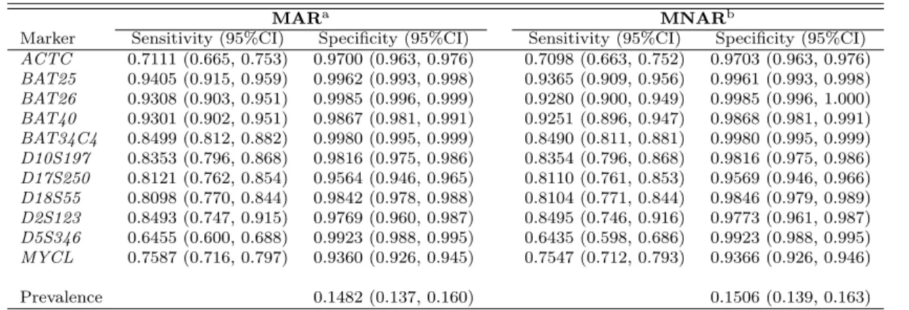
Applying the proposed method to the C-CFR data we obtained the point estimates for θ, which includes π1, Sej, Spj as well as r1j, r0j for all 11 biomarkers, and their standard errors (SE). The 95% CIs are then obtained from point estimates and SEs. The results for θ under different missing assumptions are presented in Table 2.3. The point estimates with 95% CIs under the MNAR assumption are almost the same with those under the MAR assumption. The slight difference is caused by introducing columns of 1 for missing indicator of δij for our method.
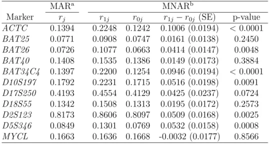
The estimates for missing probabilities are presented in Table 2.6. Under the MNAR assumption, we can see that for some testsr1j andr0j are quite different while for others they are very close. Generally r1j tends to be greater than r0j (the only exception is for MYCL). The reason is probably that non-diseased patients are more likely to have negative test results, and patients with negative test results are more willing to take additional tests (hence smaller missing probabilities) to confirm they do not have the disease. As expected,rj under the MAR assumption falls betweenr1j and r0j.
The log-likelihood ratio statistic (LRS) is found to be −2(l(˜θ|T,∆)−l(ˆθ|T,∆))= −2×(−21407.85−(−21166.83))= 482.04 > χ2
0.95,11, where χ20.95,11 = 19.675 is the
95th percentile of the the χ2 distribution with d.f.=11. Therefore we reject the null
colon cancer. To tell whether r1j and r0j are significantly different for each test j, we calculated p-values based on Wald statistic, which is calculated as r1j−r0j
SEr1j ,r0j where
SEr1j,r0j =
p
Varr1j + Varr0j −2Covr1j,r0j. These nominal p-values can be adjusted for
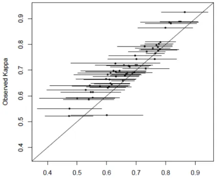
multiplicity using Bonferroni correction (multiply byJ = 11). The results suggest that the MNAR assumption is more plausible than the MAR assumption for our case study. Figure 2.1 plots the model based Kappa statistics versus observed Kappa statistics as a graphical check for conditional independence assumption. The model based Kappa statistics in Figure 2.2(a) are derived from diagnostic accuracy estimates under the MAR assumption, and the model based Kappa statistics in Figure 2.2(b) are from the MNAR assumption. Not surprisingly, these two figures look similar due to the resemblance of diagnostic accuracy estimates under the two assumptions. In both figures, all of the 95% simultaneous confidence intervals of model-based Kappa contain the observed Kappa statistics. Hence these figures fail to reject the null hypothesis of conditional independence assumption.
2.5
Simulation Studies
To further investigate the performance of the proposed methods, 10000 simulations were run. For each simulation, we generateN = 3,500 observations (chosen to be close to the sample size of the real data, N = 3,487) with J = 5 tests including missing indicators for each test under three different missing pattern assumptions. The true values of prevalence is set to beπ1 = 0.2, close to the estimates from the C-CFR study.
The true values of sensitivity and specificity are set to be close to estimates for the five NCI-recommended microsatellite sequence panels (BAT25,BAT26,D17S250,D2S123,
0,1 from a binomial distribution with Se and (1−Sp) as the binomial p under the assumption that Ti are independent given Di. Finally, we randomly assign missing indicator ∆i to each test results considering the three missing scenarios. Simulation results are listed in Table 2.1.
We first simulated the missingness of test results under the MCAR assumption. All five tests were randomly assigned a missing indicator (1 = observed; 0 = missing), through a binomial distribution, independent of any other missing or observed values. The missing probabilities of the five tests (r1,· · · , , r5) are 0.274, 0.090, 0.251, 0.023,
0.089 subsequently, which were randomly selected from a uniform distribution bounded by (0,0.35). Secondly, under the MAR assumption, we let the missing patterns of Test 4 and Test 5 depend on some fully-observed test results. ∆i1 and ∆i2 all equal to 1
(the first two tests have no missing value); ∆i3 are randomly generated from a binomial
distribution with a missing probability of 0.2 (the third test is MCAR); ∆i4 is randomly
generated from a binomial distribution with missing indicator ∆i4 depending on Ti1
through equationlogit(P(∆i4 = 1|Ti1)) =α+β1Ti1; and ∆i5is randomly generated from
a binomial distribution with missing indicator ∆i5 depending on Ti1 and Ti2 through
equationlogit(P(∆i5 = 1|Ti1, Ti2)) = α+β1Ti1+β2Ti2. The regression coefficients are
set toα=−1.5,β1 =−4,β2 = 2. Lastly, for the MNAR assumption, Test 4 and Test 5
depend on a subset of unobserved tests or disease status. ∆i1, ∆i2 and ∆i3are generated
following the same settings as for the MAR assumption. ∆i4 is randomly generated
from a binomial distribution with missing indicator ∆i4 depending on partially-observed
Ti3 through equation logit(P(∆i4 = 1|Ti1, Ti3)) = α + β3Ti3, and ∆i5 is randomly
generated from a binomial distribution with missing indicator ∆i5 depending on both
Ti3 and unobservable disease status D through equation logit(P(∆i5 = 1|Ti3, D)) =
α+β3Ti3+β5D, where α=−1.5, β3 = 0.75, β5 = 0.7.
probabilities above 95%. The SE estimates are also very close to the standard deviations from point estimates ofπ1,SeandSp. The average missing probability for Test 1 under
MCAR assumption is the highest (almost 30% observations missing), yet the coverage probability is still very good (>95%) for its sensitivity and specificity. Under the MAR assumption, the coverage probabilities for π1 and Se is a bit poorer than the MCAR
assumption albeit the coverage probabilities for Sp is almost undifferentiable between the two tests. The missing probabilities under the MAR assumption vary between [0.004,0.182] for Test 4, and [0.004,0.622] for Test 5. The average missing probabilities under the MAR assumption are 0.136 for Test 4 and 0.183 for Test 5. Although the missing probabilities for Test 5 can be as high as 0.622, the coverage probability for Test 5 is very good (> 95%) for both sensitivity and specificity. Our method is well suitable for both the MCAR and MAR assumptions. Under the MNAR assumption, the missing probabilities vary between [0.182,0.321] for Test 4, and [0.182,0.488] for Test 5. The average missing probabilities under the MNAR assumption are 0.217 for Test 4 and 0.250 for Test 5, both greater than those under the MAR assumption. Generally speaking the coverage probabilities under the MNAR assumption are not compromised much as all are above 94%. We do observe that the coverage probability for Sp is consistently smaller comparing to the MAR assumption. This may be explained by the missingness of Test 4 only depends on Test 3 (which is MCAR), while the missingness of Test 5 depends on latent disease status in addition to Test 3. As a sensitivity analysis, we did another simulation for the MNAR assumption with everything the same except that ∆i5 depends on Ti3 and Ti5 through equation logit(P(∆i5 = 1|Ti3, Ti5)) =
α+β3Ti3 +β5Ti5. Our method did not handle Test 5 estimation very well: although
when the cause of a missing test lies in the value of another test or the true disease status, whereas MNAR can cast doubt on our estimation if the cause of a missing is the value of the missing test itself.
We also conducted a simulation to assess estimation of missing probabilities under the new assumption for MNAR, where the missingness of each test depends on the unknown disease status. The missing probabilities for Test 1 through Test 5 were subsequently set to (0.1,0.1,0.2,0.2,0.3) for r1 and (0.1,0.2,0.4,0.6,0.8) for r0, while
π1, Se and Sp hold the same values as before. The estimates of r1 and r0 along with
π1, Se and Sp are obtained simultaneously with coverage probabilities varying from
94.8% to 95.8%. Our method is once more shown to handle different missing scenarios fairly well.
2.6
Discussion
bias throughout all tests. In conclusion, our method is straightforward to comprehend and simple to implement for diagnostic studies involving multiple conditionally inde-pendent tests with moderate percentages of missing data and without a gold standard. It has the potential to improve public health by facilitating the diagnosis of cancer and other prevalent diseases.
Common methods such as case deletion, maximum likelihood estimation, multiple imputation, etc. are valid for MCAR and MAR but cannot handle MNAR without explicitly modeling the missing pattern. Two possible models to account for MNAR data are selection models (Heckman, 1979) and pattern mixture models (Little, 1993). These models are complicated and require substantial statistical knowledge and soft-ware experience, yet their validity is not easily justifiable and sometimes questionable. Methodological development to cope with missing data under the MNAR assumption is beyond our current scope but would be considered for future research.
Figure 2.1: Plot of Observed vs. Model Based Kappa
0.4 0.5 0.6 0.7 0.8 0.9
0 .4 0 .5 0 .6 0 .7 0 .8 0 .9
Model Based Kappa
O b se rv e d Ka p p a ● ● ● ● ● ● ● ● ● ● ● ● ● ● ● ● ● ● ● ● ● ● ● ● ● ● ● ● ● ● ● ● ● ● ● ● ● ● ● ● ● ● ● ● ● ● ● ● ● ● ● ● ● ● ●
(a) Under the MAR Assumption
0.4 0.5 0.6 0.7 0.8 0.9
0 .4 0 .5 0 .6 0 .7 0 .8 0 .9
Model Based Kappa
O b se rv e d Ka p p a ● ● ● ● ● ● ● ● ● ● ● ● ● ● ● ● ● ● ● ● ● ● ● ● ● ● ● ● ● ● ● ● ● ● ● ● ● ● ● ● ● ● ● ● ● ● ● ● ● ● ● ● ● ● ●
(b) Under the MNAR Assumption
Note: Dots and lines are model based Kappa statistics with their corresponding 95% simultaneous
Table 2.2: Number of Subjects by Frequency of Missing Test Results
Table 2.3: Estimates and 95% CIs of Sensitivity, Specificity, and Prevalence from Dif-ferent Models
MARa MNARb
Marker Sensitivity (95%CI) Specificity (95%CI) Sensitivity (95%CI) Specificity (95%CI)
ACTC 0.7111 (0.665, 0.753) 0.9700 (0.963, 0.976) 0.7098 (0.663, 0.752) 0.9703 (0.963, 0.976)
BAT25 0.9405 (0.915, 0.959) 0.9962 (0.993, 0.998) 0.9365 (0.909, 0.956) 0.9961 (0.993, 0.998)
BAT26 0.9308 (0.903, 0.951) 0.9985 (0.996, 0.999) 0.9280 (0.900, 0.949) 0.9985 (0.996, 1.000)
BAT40 0.9301 (0.902, 0.951) 0.9867 (0.981, 0.991) 0.9251 (0.896, 0.947) 0.9868 (0.981, 0.991)
BAT34C4 0.8499 (0.812, 0.882) 0.9980 (0.995, 0.999) 0.8490 (0.811, 0.881) 0.9980 (0.995, 0.999)
D10S197 0.8353 (0.796, 0.868) 0.9816 (0.975, 0.986) 0.8354 (0.796, 0.868) 0.9816 (0.975, 0.986)
D17S250 0.8121 (0.762, 0.854) 0.9564 (0.946, 0.965) 0.8110 (0.761, 0.853) 0.9569 (0.946, 0.966)
D18S55 0.8098 (0.770, 0.844) 0.9842 (0.978, 0.988) 0.8104 (0.771, 0.844) 0.9846 (0.979, 0.989)
D2S123 0.8493 (0.747, 0.915) 0.9769 (0.960, 0.987) 0.8495 (0.746, 0.916) 0.9773 (0.961, 0.987)
D5S346 0.6455 (0.600, 0.688) 0.9923 (0.988, 0.995) 0.6435 (0.598, 0.686) 0.9923 (0.988, 0.995)
MYCL 0.7587 (0.716, 0.797) 0.9360 (0.926, 0.945) 0.7547 (0.712, 0.793) 0.9366 (0.926, 0.946)
Prevalence 0.1482 (0.137, 0.160) 0.1506 (0.139, 0.163)
Table 2.4: Estimates and 95% CIs of r1j, r0j, and rj under Different Missing Data Assumptions
MARa MNARb
Marker rj r1j r0j r1j −r0j (SE) p-value
ACTC 0.1394 0.2248 0.1242 0.1006 (0.0194) <0.0001
BAT25 0.0771 0.0908 0.0747 0.0161 (0.0138) 0.2450
BAT26 0.0726 0.1077 0.0663 0.0414 (0.0147) 0.0048
BAT40 0.1408 0.1535 0.1386 0.0149 (0.0173) 0.3884
BAT34C4 0.1397 0.2200 0.1254 0.0946 (0.0194) <0.0001
D10S197 0.1792 0.2231 0.1715 0.0516 (0.0198) 0.0091
D17S250 0.4193 0.4554 0.4129 0.0425 (0.0237) 0.0724
D18S55 0.1342 0.1508 0.1313 0.0195 (0.0172) 0.2573
D2S123 0.8173 0.8606 0.8097 0.0509 (0.0168) 0.0025
D5S346 0.0849 0.1301 0.0769 0.0532 (0.0158) 0.0008
MYCL 0.1663 0.1636 0.1668 -0.0032 (0.0177) 0.8566 aMissingness does not depend on latent disease status.
bMissingness depends on latent disease status.
Note: rjdenotes missing probability for each test;r1jandr0jdenote missing probabilities for diseased
Chapter 3
Conditional Dependence
Assumption
3.1
Introduction
Begg and Greenes, 1983; Harel and Zhou, 2007; He and McDermott, 2012; Lin et al., 2006; Yu et al., 2010; Zhou, 1998) and the non-ignorable (Baker, 1995; Geloven et al., 2012; Harel and Zhou, 2007; Kosinski and Barnhart, 2003b,a; Zhou, 1993) missing data assumptions.
Greenberg, 1998; Xu and Craig, 2009).
A PLC model is a version of LCA in which specified threshold locations discretize a latent continuous variable into different regions that correspond to observed response levels. Qu et al. (1996) developed a special PLC model, called the Gaussian random effects model, because conditional dependence between tests is addressed by subject-specific random effects in a standard Gaussian distribution that links the observed test results to the latent disease status through a probit model. Qu and Hadgu (1998) extended the Gaussian random effects model to a generalized linear mixed model with a hybrid algorithm that combined the EM algorithm and the Newton-Raphson method for its ML estimates. Dendukuri and Joseph (2001) presented a Bayesian approach similar to the random effects model of Qu et al. by imposing a prior distribution to summarize the uncertainty about each parameter. However, these models simply assume that the dependence between tests is based on their having the same distribution, which is hard to justify. To relax this assumption, Uebersax (1999) proposed a PLC model that assumes a multivariate-normal distribution within each latent class so that the correlation structure can be modeled flexibly. Employing the Monte Carlo EM (MCEM) algorithm (Wei and Tanner, 1990), Chib and Greenberg (1998) obtained ML estimates for multivariate probit models with a general covariance structure. Xu and Craig (2009) further developed a PLC model to estimate diagnostic accuracy while accommodating a general correlation structure between tests using a parameter-expanded Monte Carlo EM (PX-MCEM) algorithm, which was motivated by the MCEM algorithm (Chib and Greenberg, 1998) and the parameter-expanded EM (PX-EM) algorithm (Liu et al., 1998). A TLC model is a special version of the PLC model when the two covariance matrices are restricted to be diagonal.
missing); (ii) a gold standard is never applied or does not exist (totally missing). Po-leto et al. (2011) presented a scenario in which all subjects are evaluated with a gold standard and one of the three imperfect tests under evaluation, whereas the other two imperfect tests are not always performed. They used a two-stage hybrid approach (i.e., ML in stage one and weighted least squares in stage two) to estimate the diagnostic accuracy of the three imperfect tests. To our knowledge, when a gold standard is to-tally missing, there is no study that has evaluated the diagnostic accuracy of multiple correlated diagnostic tests with excessive missing data. Motivated by the Colon Cancer Family Registry (C-CFR) study (Section 2), we extended the PLC models under the conditional dependence assumption to evaluate the prevalence and diagnostic accuracy of multiple imperfect diagnostic tests with high proportions of missing data and with-out a gold standard. In addition, we also evaluated the correlation between these tests through a general correlation structure of the PLC model.
The remainder of this paper is organized as follows. Section 3.2 introduces the C-CFR study that motivated our research. Section 3.3 describes the PLC-based method-ology of estimating diagnostic accuracy and correlation matrices, as well as the boot-strap approach for estimating their standard errors. Section 3.4 summarizes the results of simulation studies with different missing data assumptions and examines the finite sample properties of the proposed model. Section 3.5 presents the preliminary analyses of the C-CFR data. Finally, section 3.6 concludes with an extensive discussion.
3.2
Motivating Example
pathway that repairs the mismatches in the genome that occur during cell duplication. It is estimated that 600,000 individuals in the United States have HNPCC. These indi-viduals have a substantially increased (up to 80%) lifetime risk of developing cancer in the colorectum and other sites when compared to the general public. Mutation analysis of the MMR genes may be considered a gold standard for HNPCC diagnosis. How-ever its high cost ($2,000 - $3,000 per individual) precludes its broad use in HNPCC screening. A relatively inexpensive alternative ($200 - $300 per individual) (Thibodeau, 1981) seeks to identify a high level of microsatellite instability (MSI), the amplification or deletion within microsatellites (common and normal repeated sequences of DNA). Since the establishment of a consensus definition of MSI and unifying criteria for its measurement in 1998 (Boland et al., 1998), MSI biomarker tests have been used regu-larly as part of the international guidelines for HNPCC diagnosis (Umar et al., 2004). Therefore it is of great interest from a public health perspective to evaluate the diag-nostic accuracy of MSI biomarkers for early detection and prevention of HNPCC.
The NCI C-CFR study is an international consortium of six centers in North Amer-ica and Australia that was formed to support studies on the etiology, prevention, and clinical management of colorectal cancer (Newcomb et al., 2007). The C-CFR data include test results of 11 MSI biomarkers (namelyBAT25, BAT26,BAT40,BAT34C4,
our methodology research, which is to be introduced in the next section.
3.3
Statistical Methods
3.3.1
PLC Model Parameters Specification and Expansion
Suppose that we have a total ofN subjects andJ binary tests. LetDi =d(d= 1,0) represent the latent variable for disease status (1=Yes, 0=No) of the ith subject (i = 1,· · · , N,). Letπd =P r(Di =d) denote the probability of disease/no disease of the the
ith subject (π1 is the prevalence). Let tij be the result of the jth test of the ith subject. Notice that due to missing values, the test results are not in the typical “binary” fashion with three possible values, i.e., 1=positive, 0=negative, 99=missing. Let δij be the indicator of whether the ith subject has been tested by the jth test (1=tested, 0=not tested). Ti = (ti1,· · · , tiJ) and ∆i = (δi1,· · · , δiJ) represent all the test results and missing indicators of the ith subject. Under the conditional dependence assumption, the similarity between tests of the ith subject is explained by some Gaussian latent variable Zi = (zi1,· · · , ziJ)0, which has a multivariate normal distribution conditional onDi, i.e. Zi|Di =d∼NJ(µd,Σd) with mean vectorµdand variance-covariance matrix Σd = {σ
(d)
ij }. We assume zij > 0 when tij = 1; zij <= 0 when tij = 0; zij could take any value within (−∞,∞) whentij is missing. The probability of observing (Ti, ∆i) is obtained by integrating overZi:
P(Ti,∆i|Di =d, µd,Σd) = Z
Bi1 · · ·
Z
BiJ
where the integration interval of each test is
Bij =
(−∞,0] iftij=0 (0,∞) iftij=1
(−∞,∞) iftij=99, i.e. δij = 0
(3.1)
However we are unable to find a fixed solution for the model parameters (µd,Σd) since they are not identifiable. One way to overcome this challenge is to restrict the variance-covariance matrix Σdto correlation matrixRdwith all diagonal elements equal to 1 and all off-diagonal elements between [−1,1], and then re-parameterize µd to ad (Chib and Greenberg, 1998). It can be shown that the sensitivity and specificity of the
jth test are Se
j = Φ(a1j) and Spj = Φ(−a0j), respectively. Let θ = (π1, a1, R1, a0, R0)
denote the vector of all 1+2J+2×J(J2−1) =J2+J+1 unique parameters. Assume that we knowZi andDi in addition to the observed data (Ti, Di), and assume that, for any pair of two tests, there are at least some subjects with both test results present. (For the C-CFR data set, this is of no concern because 219 subjects have all 11 test results present.) By Bayes’ theorem, the log-likelihood of complete data Yi = (Ti,∆i, Zi, Di) is
logLc(θ) = logL(θ|Ti,∆i, Zi, Di) = log
N Y
i=1
{P(Ti,∆i|Zi, Di, θ)}
= log N Y
i=1
{P(Di|π1)P(Zi|Di, a1, R1, a0, R0)P(Ti,∆i|Zi, a1, R1, a0, R0)}
Rd) = QJ
i=1I(zij ∈Bij), P(Di|π1) = πd1i(1−π1)(1−di), the log-likelihood becomes
logLc(θ) = log N Y
i=1
{πdi
1 (1−π1)(1−di)φJ(Zi;a1, R1)diφJ(Zi;a0, R0)(1−di)
J Y
i=1
I(zij ∈Bij)}
= N X
i=1
{dilog(π1) + (1−di)log(1−π1) +dilog(φJ(Zi;a1, R1))
+(1−di)log(φJ(Zi;a0, R0)) +
J X
i=1
log(I(zij ∈Bij))}
3.3.2
ML Estimation Using the Monte Carlo EM Algorithm
the approximation error since one can increase the Monte Carlo sample size until the desired accuracy is obtained.
The MCEM algorithm is well suited for our C-CFR case study: first, we are deal-ing with missdeal-ing test results as well as the latent disease status; secondly, our PLC model involves an intractable E-step due to the high-dimensional integration incurred by the 11 tests. However, the M-step does not have a closed-form solution when the variance-covariance matrices are restricted to be correlation matricesRd. Thus we need to expand the parameters as µd =V
1 2
d ad and Σd =V 1 2 d RdV
1 2
d following the PX-EM al-gorithm by Liu et al. (1998). Vd is a J ×J diagonal matrix with all diagonal elements positive. The parameter vector becomes β = (π1, µ1,Σ1, µ0,Σ0) and the log-likelihood
becomes
logLc(β) = log N Y
i=1
{πdi
1 (1−π1)(1−di)φJ(Zi;µ1,Σ1)diφJ(Zi;µ0,Σ0)(1−di)
J Y
i=1
I(zij ∈Bij)}
= N X
i=1
{dilog(π1) + (1−di)log(1−π1) +dilog(φJ(Zi;µ1,Σ1))
+(1−di)log(φJ(Zi;µ0,Σ0)) +
J X
i=1
log(I(zij ∈Bij))}
Substituting the joint density functions of the multivariate normal distribution
φJ(Zi;µd,Σd) = (2π)J/21|Σ
d|1/2exp{−
1
2(Zi −µd)
0Σ−1
d (Zi − µd)}(d = 1,0) into logLc(β) we have the final log-likelihood function of the complete data
logLc(β) = log N Y
i=1
{πdi
1 (1−π1)(1−di)φJ(Zi;µ1,Σ1)diφJ(Zi;µ0,Σ0)(1−di)
J Y
i=1
= N X
i=1
{dilog(π1) + (1−di)log(1−π1)
−1
2log|Σ1|di− 1
2di(Zi−µ1)
0
Σ−11(Zi−µ1)−
J
2log(2π)di −1
2log|Σ0|di− 1
2di(Zi−µ0)
0
Σ−01(Zi−µ0)−
J
2log(2π)di +
J X
i=1
log(I(zij ∈Bij))} (3.2)
The M-step is to solve the score equations after taking expectations conditional on the complete data:
0 = N X
i=1
E[{di
π1
− 1−di 1−π1
}|Ti,∆i, β(n)]
0 = N X
i=1
E[{diZi−diµ1}|Ti,∆i, β(n)]
0 = N X
i=1
E[{(1−di)Zi−(1−di)µ0}|Ti,∆i, β(n)]
0 = N X
i=1
E[{−1 2Σ
−1 1 di+
1 2Σ
−1
1 (Zi−µ1)(Zi−µ1)0Σ1−1di}|Ti,∆i, β(n)]
0 = N X
i=1
E[{−1 2Σ
−1
0 (1−di) + 1 2Σ
−1
The solutions are:
π(1n+1) = 1
N
N X
i=1
E[di|Ti,∆i, β(n)]
µ(1n+1) = PN
i=1E[diZi|Ti,∆i, β (n)]
PN
i=1E[di|Ti,∆i, β(n)]
µ(0n+1) = PN
i=1E[(1−di)Zi|Ti,∆i, β(n)] PN
i=1E[(1−di)|Ti,∆i, β(n)] Σ(1n+1) =
PN
i=1E[di(Zi−µ1)(Zi−µ1)0|Ti,∆i, β(n)] PN
i=1E[di|Ti,∆i, β(n)]
Σ(0n+1) = PN
i=1E[(1−di)(Zi−µ0)(Zi−µ0)
0|T
i,∆i, β(n)] PN
i=1E[(1−di)|Ti,∆i, β(n)]
They are simplified for d= 1,0 as
π(1n+1) = 1
N
N X
i=1
E[di|Ti,∆i, β(n)]
µ(dn+1) = PN
i=1E[d
d
i(1−di)1−dZi|Ti,∆i, β(n)] PN
i=1E[ddi(1−di)1−d|Ti,∆i, β(n)] Σ(dn+1) =
PN i=1E[d
d
i(1−di)1−d(Zi−µd)(Zi−µd)0|Ti,∆i, β(n)] PN
i=1E[ddi(1−di)1−d|Ti,∆i, β(n)] =
PN
i=1E[ddi(1−di)1−dZiZi0|Ti,∆i, β(n)] PN
i=1E[d
d
i(1−di)1−d|Ti,∆i, β(n)]
−µ(dn+1)(µ(dn+1))0 (3.3)
The estimates for ad and Rd can be derived by reducing the expanded parameter through Ud (a diagonal matrix with diagonal elements equal to those of Σ(dn+1)):
a(dn+1) = U−
1 2 d µ
(n+1)
d
R(dn+1) = U−
1 2 d Σ
(n+1)
d U
−1 2
d (3.4)
For the E-step we compute the conditional expectations of the expanded com-plete data sufficient statistics, i.e. PNi=1E[di|Ti,∆i, β(n)], PNi=1E[diZi|Ti,∆i, β(n)], PN
i=1E[diZiZ
0
i|Ti,∆i, β(n)], PNi=1E[(1 − di)Zi|Ti,∆i, β(n)], and PNi=1E[(1 − di)ZiZi0 |Ti,∆i, β(n)] via Markov chain Monte Carlo (MCMC) routines such as the Gibbs and Metropolis-Hastings samplers. For computation efficiency, we grouped subjects by K
distinctive response profiles with nk subjects for each response profile. (Subjects with the same results for allJ tests are said to have the same response profile.) With three possible test results (1, 0, missing), the total number of possible profiles for J tests is 3J−1. It is unlikely for the observed data to contain all possible profiles since 3J−1 increases exponentially with J. For the C-CFR data, the actual number of profiles observed is K = 887 but the total number of possible profiles is 311−1 = 177,146. It
is reasonable to speculate that the 177,146−887 = 176,259 missing profiles are due to ignorable missing data mechanism, i.e. there is no clinical or other logical consideration that precludes a response profile from occurring.
We adopt Xu and Craig’s (2009) sampling algorithm, which reduces a truncated multivariate normal distribution to a computationally much easier problem involving a series of univariate truncations. We proceed as follows:
• Begin with a set of arbitrary starting values for the parameter θ(0) = β(0) =
(π1(0), a(0)1 , a0(0), Rd(0), R(0)0 ) and the latent variableZk(0) = (zk1,· · · , zkJ)0(k = 1,· · · ,
K). For the first MC sample m = 1, generate d(0)k from Bernoulli(p(0)k ), where
p(0)k = π (0) 1
π1(0)+(1−π(0)1 )r and r=
φJ(z(0)k ;a(0)0 ,R (0) 0 ) φJ(z
(0)
k ;a
(0) 1 ,R
(0) 1 )
.
• Generate Zk(1) given d(0)k = d from a truncated normal distribution T N(µ∗, σ∗2)
where the integration interval isBkj,σ∗2 = (R−11
d )j,j,µ
∗ =a
dj−σ∗2(R−d1)j,−j(Zk,−j−
ad,−j). Draw each zkj(j = 1,· · · , J) from the distribution of zkj conditioned on all other variables, making use of the most recent values and updating zkj with its new value as soon as it has been drawn, i.e. drawzk(1)1 from [zk1|z
(0)
k2,· · · , z (0)
drawzk(1)2 from [zk2|z (1)
k1, z (0)
k3,· · · , z (0)
kJ],· · ·, draw z
(1)
kJ from [zkJ|z
(1)
k1,· · · , z (1)
k,(J−1)].
• Repeat the above simulation steps form={2,· · · , M}to generateM samples of
dkandZk. The conditional expectations of the expanded complete data sufficient statistical are estimated by averaging over the M Monte Carlo samples, e.g., PN
i=1E[diZi|Ti,∆i, β
(n)] = PK
i=1E[nkdkZk|Ti,∆i, β
(n)] = 1
M PM
m=1
PK k=1nkd
(m)
k
Zk(m). Substituting the estimated conditional expectations into 3.3, we derive parameter estimates β(1) = (π(1)
1 , µ (1) 1 , µ
(1) 0 ,Σ
(1) 1 ,Σ
(1)
0 ), and subsequently θ(1) =
(π1(1), a(1)1 , a(1)0 , R1(1), R(1)0 ). This completes the first iteration l = 1. θ(1) and Zk(M)
(the last MC sample) will be starting values for the next iteration.
• Repeat the above PX-MCEM algorithm steps for l = 2,3,· · · until the conver-gence at l = L, i.e. the difference between θ(L) and θ(L−1) is consecutively less
than a preset tolerance for several iterations. Then, we have the final estimates
θ(L), which converge to the true parameter valuesθ by the law of large numbers.
To control the between-simulation variability known as Monte Carlo error (MCE), a large MC sample sizeM (typically at least 10,000) is preferred but it may quickly be-come computationally burdensome. It is advisable to implement a smallM for the first few iterations whenθ(l) is far from the true parameter valuesθ, and increaseM for later
iterations whenθ(l) moves closer toθ(Wei and Tanner, 1990). For example, McCulloch developed MCEM algorithms that increase M linearly (1994) and nonlinearly (1997) with the number of iterations. We used a more efficient cumulative MCEM algorithm (Kou et al., 1998) by fixing M as a relatively small number (e.g. M = 1500) for all iterations. It utilizes MC samples from the current iteration as well as an adaptively increasing number of previous iterations, so that simulations from previous iterations are not wasted.
We thinned the chain by saving everyothsimulated sample from each sequence. Another issue arises when the MC samples at the beginning of the chain do not represent the desired distribution accurately. We discarded the initial MC samples of each iteration for early EM iterations during the burn-in period.
The adequacy of the model can be checked by plotting all J(J2−1) pairwise correlation residuals (Qu et al., 1996). The correlation coefficient between any two teststij andtij0
is √ P(tij=1,tij0=1)−P(tij=1)P(tij0=1)
P(tij=1)(1−P(tij=1))P(tij0=1)(1−P(tij=0))
. For observed pairwise correlation coefficients,
P(tij = 1) =
PN
i=1tij
N and P(tij = 1, tij0 = 1) =
PN
i=1tijtij0
N . For model-based pairwise correlation coefficients, P(tij = 1) = P10πd
R∞
0 φj(Zi;µd,Σd)dzij and P(tij = 1, tij0 =
1) = P1
0πd
R∞
0
R∞
0 φj,j0(Zi;µd,Σd)dzijdzij0. The residuals are the differences between
the observed and model-based pairwise correlation coefficients.
3.3.3
Starting Values for the PX-MCEM Algorithm
When the loglikelihood function is concave and unimodal over the entire parameter space, the PX-MCEM algorithm converges to the unique MLE θ(L) from any set of
starting values. In that senseθ(0) = (π(0) 1 , a
(0) 1 , a
(0) 0 , R
(0) 1 , R
(0)
0 ) can be selected arbitrarily
However, multiple maxima often exist, and the PX-MCEM algorithm is not guar-anteed to converge to a unique global maximum. One suggestion is to try a variety of starting values to examine whether a global maxima is reached rather than a local maximum. This becomes impractical due to the computational intensity of the PX-MCEM algorithm, as well as the large number of tests and subjects for the C-CFR data. Conversely, the TLC model is much more efficient computationally. It has been shown that the TLC model is adequate even with conditionally dependent tests when the accuracies of the tests are high or when the tests are weakly dependent (Hui and Zhou, 1998; Georgiadis et al., 2003). In this paper we extended the TLC model under the conditional independence assumption to allow for missing data, and we used the model’s estimates of the parameter as our starting values. Assuming that the ignorable missing data mechanism is tenable, the probability of observing (Ti,∆i) for subjectiis
pθ(Ti,∆i) =
1
X
d=0
πdhid (3.5)
where
hi1 =
J Y
j=1
Setijδij
j (1−Sej)(1−tij)δij
hi0 =
J Y
j=1
(1−Spj)tijδijSp
(1−tij)δij
j .
Let γ = (π1, Se1,· · · , SeJ, Sp1,· · · , SpJ). Start with some arbitrary starting values
the score equations as:
0 = N X
i=1
E[{di
π1
− 1−di 1−π1
}|Yi, γ(n)]
0 = N X
i=1
E[{ditijδij
Sej
− diδij −ditijδij 1−Sej
}|Yi, γ(n)]
0 = N X
i=1
E[{(1−di)(1−tij)δij
Spj
− (1−di)tijδij 1−Spj
}|Yi, γ(n)]
whereYi = (Ti,∆i, Di) are the complete data. We computeE[di|Yi, γ(n)] in the E-step and derive γ(n+1). Iterating EM steps until convergence, we get the final estimates ˆγ. After transformation ˆa1j = Φ−1( ˆSej) and ˆa0j =−Φ−1( ˆSpj) are our starting values for
a1j and a0j to initiate the PX-MCEM algorithm aforementioned. Simulation studies indicate great coverage probability for ˆSej and ˆSpj when the missing rate of test j is not too high and the conditional independence assumption holds. When the condi-tional independence assumption is relaxed to the condicondi-tional dependence assumption,
ˆ
Sej and ˆSpj are still reasonably close to the true values. The TLC model converts oth-erwise arbitrary starting values to the best available starting values. Nevertheless, the TLC model does not estimate R1 and R0, so their starting values have to be selected
arbitrarily.
3.3.4
Bootstrap Method for Standard Errors
MLEs with good coverage, even if the model is misspecified or if the model assumptions, such as the ignorable missing-data assumption, are invalid (Efron, 1994).
The bootstrap method is employed to estimate the SE of the ML estimate of θ. We randomly drewB bootstrap samples of size N from observed dataT1,· · · , TN with replacement. Then, the PLC model was applied to each bootstrap sample to get the ML estimates (ˆθ(1),· · · ,θˆ(B)). The bootstrap estimate of θ is ˆθ
boot =
PB
b=1θˆ(b)
B and the SE estimate is ˆSEboot =
qPB
b=1(ˆθ(b)−θˆboot)2
B−1 . It has been demonstrated that B = 200 is
required if the bootstrap distribution is approximately normal (Efron, 1994).
3.4
Simulation Studies
We assessed the performance of the PLC model when fitting simulated data sets from different missing data mechanisms. Each simulation study consists of S = 500 simulations. Each simulation generated a simulated data set with N = 3,500 sub-jects and J = 5 tests. The true parameter values were set to π1 = 0.2, Se =
(0.7,0.9,0.8,0.6,0.75), and Sp = (0.9,0.85,0.9,0.9,0.8). All test results are condi-tional dependent, i.e., the correlation coefficients between any two tests are 0.6 for diseased subjects and 0.45 for non-diseased subjects. For simulated data sets under the MCAR mechanism, all tests were assigned randomly δij = 1 or 0 with P(δij = 1) = (0.95,0.9,0.8,0.5,0.1). For simulated data sets under the MAR and MNAR mech-anisms, ti1 and ti2 are always observed, whereas ti3 has P(δi3 = 1) = 0.8. Under
the MAR mechanism, ti4’s missing probability depends on ti1 through logit(P(δi4 =
1|ti1)) = α+β1ti1;ti5’s missing probability depends onti1 andti2 through logit(P(δi5 =
1|ti1, ti2)) = α0 +β10ti1 +β2ti2. Under the MNAR mechanism, ti4’s missing
probabil-ity depends on ti1 and ti3 through logit(P(δi4 = 1|ti1, ti3)) = α+β1ti1 +β3ti3; ti5’s
missing probability depends on ti1, ti2, ti3 and unobservable disease status Di through
models are set toα = 1.5,β1 =−2.5,β2 =−2,β3 =−1.5,β4 =−0.7,α0 = 2,β10 =−2,
β30 =−3. Under the MAR mechanism, the missing probabilities vary from 0.18 to 0.73 for ti4 and from 0.12 to 1.00 for ti5. The average missing probabilities are about 30%
for T4 and 40% for T5. Under the MNAR mechanism, the missing probabilities vary
from 0.18 to 0.92 forti4 and from 0.12 to 1.00 forti5. The average missing probabilities
for T4 and T5 are 40% and 50% respectively.
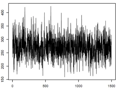
The PLC model’s estimates were obtained from each simulated data set, and the mean and standard deviation (SD) of the estimates were calculated. For each EM iteration, 3000 Gibbs sampler iterations were simulated. A burn-in of 1000 MC samples was implemented for the initial 10 EM iterations. Thinning of the chains was performed by saving every 2nd MC sample, which resulted in 1500 MC samples for each EM iteration. Thinning decreases the correlation of the chain at the cost of increasing the number of samples required to obtain the same MC sample size. Hence, we refrained from over-thinning in the interest of computation time. We assessed convergence by visual examination. The value chosen for burn-in appears to be reasonable as it cut off all the early fluctuations. Trace plots of MC samples (e.g. PKk=1nkdk(m)Zk(m)) versus
m do not exhibit any pattern or poor mixing of MCMC. We also plotted cumulative parameter estimatesθ(l) against the PX-MCEM algorithm iteration l, which stabilized
(leveled off to a flat line) within 100 EM iterations. According to the convergence checks, our simulation settings will likely suffice.
Histograms of the bootstrap samples demonstrated a bell-shaped curve that was ap-proximately Gaussian. We also ran the Shapiro-Wilk test for each bootstrap sample and failed to reject the null assumption of normality, with almost all p-values being less than 0.05. The SE estimates closely match the SD estimates. All these results indicate good behavior of the bootstrap method. To explore the effect of increasing simula-tion size S and/or bootstrap sample size B, we did sensitivity studies with S = 400 and B = 400. The results of these studies do not show much improvement. To save computational time, we stick with S= 200 and B = 200 for all simulation studies.
Table 3.1 summarizes the simulation results when the true parameter values as used as the starting values. Under both the MCAR and MAR mechanisms, the PLC model gave unbiased estimates with good coverage probabilities for all parameters (all above 90% and most around 95%). Under the MNAR mechanism, the coverage probabilities are slightly worse forSe5 (88.2%). The PLC model is robust to data sets with abundant
missing values (e.g., the missing probabilities ofti5 are 90% for MCAR, 40% for MAR,
and 50% for MNAR) when the starting values are very close to the true values. For our proposed method, we fit the TLC model first and used the parameter estimates as starting values for prevalence and diagnostic accuracy. For R1 and R0,
the starting values were set to 0.5 for all off-diagonal elements. The estimates of the PLC model are considerably more accurate than the estimates of the TLC model as they move closer towards the true values. Under the MCAR mechanism, coverage probabilities for prevalence, sensitivities, and specificities are around 95% for all tests except forti5, due to its high percentage of missing values. Under the MAR and MNAR
mechanism, coverage probabilities for sensitivities and specificities are a little worse but the majority are still above 90%. Not surprisingly, the coverage probabilities are much worse for R1 and R0 due to their arbitrary starting values. It is noteworthy that the
that more data are available from non-diseased subjects for estimation of R0.
Additional simulation studies were conducted with different starting values for the PX-MCEM algorithm to illustrate their effects on parameter estimates. For example, we obtained starting values following the method of Walter and Irwig (1988), which was based on the majority opinion among multiple radiologists. The starting value of prevalence was set to the proportion of subjects with at least three positive tests among all subjects with at least three non-missing tests; the starting value of sensitivity for each test was set to the proportion of subjects with a positive result for this test among all subjects with at least three positive tests and a non-missing result for this test; the starting value of specificity for each test was set to the proportion of subjects with a negative result for this test among all subjects with no more than two positive tests and a non-missing result for this test. These starting values deviate further away from the true values than do the TLC estimates, and hence result in much poorer coverage probabilities. Essentially, the closer the starting values are to the true values, the better the PLC model performs in terms of coverage probabilities.
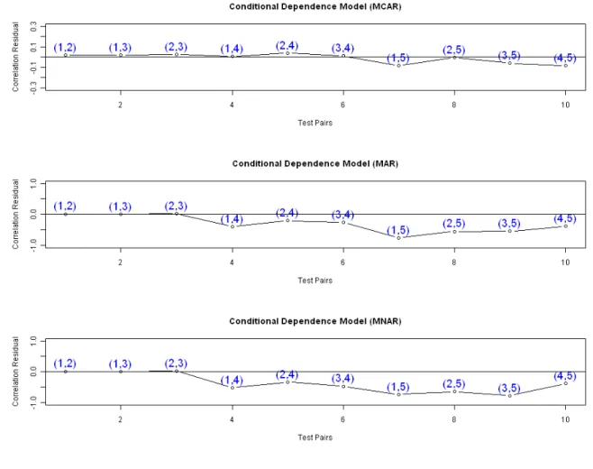
Figure 3.2 presents correlation residual plots under different missing data mech-anisms. The true parameter values for πd, µd, and Σd (d = 1,0) were used for the model-based correlation coefficients. Under the MCAR mechanism, all pairwise cor-relation residuals are close to zero, and there is no noticeable pattern, which means a good fit. Under the MAR mechanism, the correlation residuals between the two MAR tests (ti4 and ti5) and the three non-MAR tests tend to be negative, suggesting
an overestimation of such correlations. Under the MNAR mechanism, the correlation residuals between the two MNAR tests (ti4 and ti5) and the three non-MNAR tests