SPATIAL RESOLUTION IMPACTS ON DEEP CONVOLUTIONAL NEURAL NETWORKS PERFORMANCE OF LAND COVER CLASSIFICATION
Liu He
A thesis submitted to the faculty of the University of North Carolina at Chapel Hill in partial fulfillment of the requirements for the degree of Master of Arts in the Department of
Geography.
Chapel Hill 2019
© 2019 Liu He
ABSTRACT
Liu He: Spatial Resolution Impacts on Deep Convolutional Neural Networks Performance of Land Cover Classification
(Under the direction of Conghe Song)
ACKNOWLEDGEMENTS
TABLE OF CONTENTS
LIST OF TABLES ... vii
LIST OF FIGURES ... viii
LIST OF ABBREVIATIONS ... ix
CHAPTER 1: INTRODUCTION ...1
CHAPTER 2: METHODOLOGY ...8
2.1 Experimental scenarios ...8
2.2 Training data generation ...13
2.3 Deep residual fully convolutional networks (DRFCN) ...15
2.3.1 Convolutional neural networks (CNNs) ...15
2.3.2 Fully convolutional networks (FCN) ...21
2.3.3 Residual networks (ResNet) ...24
2.3.4 Depth-adaptive DRFCN...26
CHAPTER 3: RESULTS ...29
3.1 Training settings ...29
3.3 Insights of spatial resolution impacts on DRFCN ...39
CHAPTER 4: DISCUSSIONS ...47
4.1 Illustrations of DRFCN ...47
4.2 Full-training strategy ...48
4.3 Comparison to Maximum Likelihood Classification (MLC) ...50
4.4 Limitations ...51
CHAPTER 5: CONCLUSIONS ...53
LIST OF TABLES
Table
1. Reclassification lookup table conceived from NLCD 2011 scheme ...13
2. The architecture of DRFCN in adaptive layer depth ...28
3. DRFCN OA performance rankings and comparison to MLC ...39
4. DRFCN Kappa performance rankings and comparison to MLC ...39
5. The single-patch classification time and parameter volume for all 4 structures ...39
6a. The PA and UA for 1-4m scenarios ...44
6b. The PA and UA for 5-8m scenarios ...45
LIST OF FIGURES
Figure
1. The materials of this study ...12
2. The patch extraction and augmentation of training and validation datasets ...15
3. The illustration of a convolutional processing ...17
4. Visual illustrations of nonlinear functions ...18
5. The illustration of FCN end-to-end prediction framework ...24
6. The illustration of a basic block of residual learning ...26
7. The visual illustration of DRFCN structure ...27
8. The impact of spatial resolution on OA with all 4 networks structure ...34
9. The impact of spatial resolution on Kappa with all 4 networks structure ...35
10. The comparison of spatial resolution impacts between DRFCN and MLC ...36
11. The patterns of OA for validation set through training iterations ...37
12. The patterns of training loss for validation set through training iterations ...38
LIST OF ABBREVIATIONS
CNNs DL DCNNs DRFCN FCN Kappa KT Maxpool MLC NAIP NLCD OBIA OA PA ResNet ReLU ResBlk RF SVMs UA VHR
Convolutional Neural Networks Deep Learning
Deep Convolutional Neural Networks
Deep Residual Fully Convolutional Networks Fully Convolutional Networks
Kappa coefficient Kauth-Thomas
Maxpooling layer for DRFCN Maximum Likelihood Classification National Agriculture Imagery Program National Land Cover Database
Object-Based Image Analysis Overall Accuracy
Producer’s Accuracy Residual Networks Rectified Linear Units ResNet basic block Random Forest
Support Vector Machines User’s Accuracy
CHAPTER 1: INTRODUCTION
Global and regional land cover mapping has become an essential task for remote sensing scientists. An accurate land cover map is the aspiration for every land cover/land use
classification effort. However, to obtain accurate land cover products with limited labor and data, researchers must consider multiple important factors before they start their work (Smith et al. 2002; Chen et al. 2016). Image resolution is one of the major factors that significantly influence the accuracy of land cover classifications (Fisher et al. 2018; Suwanprasit et al. 2016, Mishra et al. 2015; Awuah et al. 2018). Generally, pixels of coarser resolution images, representing larger ground area, suffer from severe spectral confusion, and engender harder class separability. There is significant spectral heterogeneity among images with different spatial resolutions. Meanwhile, different classifiers using different training mechanisms to obtain information from input images. Given the advantage of deep learning neural networks that bring in the state-of-the-art accuracy for pattern recognition (Krizhevsky et al. 2012; Girshick et al. 2014), how to efficiently reach high classification accuracy with reasonable calculation cost is the main goal of this thesis.
limitation, former researchers exerted strengthens of various conventional classifiers for higher accuracy. Supervised classifiers based on statistical distribution of single-pixel spectral features, like Support Vector Machines (SVMs) (Huang et al. 2002), Random Forest (RF) (Gislason et al. 2006), and Neural Network (Kurnaz et al. 2005) approaches have generated acceptable
accuracies for medium resolution mapping. Besides, Object-Based Image Analysis (OBIA) that applies both single-pixel and contextual features have attained better precision for higher resolution image classifications (Ma et al. 2017) with abundant contextual features. Former researchers found accuracy benefits of increasing spatial resolution from medium to high resolution images due to purer single-pixel spectral features (Fisher et al. 2018; Suwanprasit et al. 2016, Mishra et al. 2015; Awuah et al. 2018). Since data with finer resolution provides more detailed contextual features, the increase of overall pixel-wise accuracy from very high spatial resolution (VHR) images is even more explicit through OBIA (Ma et al. 2017). It is hypothesized that a deeper extraction and representation of both individual and contextual features will
significantly contribute to higher classification accuracy, introducing the concept of Deep Convolution Neural Networks (DCNNs).
DCNNs is famous for its state-of-the-art accuracy that consistently out performs
layers, pooling layers, rectified linear units (ReLU) layers, and fully connected layers with coherent size and channels. With the increasing depth of layers, the size of intermediate heat maps shrinks because of strides in convolution and pooling layers that tend to synthesize
contextual features and reduce the volume of network parameters. Simultaneously, the dimension of heat maps increases to keep the structure of extracted features; the receptive field on original images corresponding to each pixel on heat maps also expands. In this, input images are
transformed into higher-dimensional hierarchical features, and finally modified by fully
connected layers into 1-D feature vectors for label prediction. Finally, each input image will be given a single specific label with the highest voted probability through classifying feature vectors. This training process repeats iteratively through massive input samples more than several thousand times. Aiming to reach the best accuracy, weights and parameters of
convolution kernel, ReLU functions, and nodes in fully connected layers are updated by certain loss function through gradient backward propagation. This network architecture brings final 1-D feature vectors unprecedented amount of single-pixel spectral features and hierarchical context features for great categorizing accuracy. However, the spatial distribution and localization of targeted object’s pixel groups in original images are relatively missed with exchange of more categorization features.
classification work, researchers have illustrated that DCNNs hold outstanding extraction ability of contextual features from the field within convolutional kernels (Li et al. 2017; Hamida et al. 2017), together with its authentic capability of extracting 1-D spectral features from
hyperspectral pixels (Slavkovikj et al. 2015; Midhun et al. 2014). However, most researchers directly migrated original DCNNs algorithms from computer vision, regardless of different requirements and conditions between land cover classification and novel benchmarks. First, DCNNs created by computer vision scientists are based on novel benchmarks (Dodge & Karam, 2016) containing training samples of natural and artificial objects like pets, vehicles, pedestrians etc. Input images are supposed to have at least one target object that occupies the majority of the center area, regardless of spatial resolution, while surrounding areas are all unlabeled
background (Russakovsky et al. 2015; Everingham et al. 2010). Thus, the loss of spatial and location features is affordable. In contrast, land cover/land use classification is usually
formulated as dense pixel-wise labeling for remotely sensed images (Mnih, 2013). Land cover mapping needs complete semantic segmentation of entire image into detailed category scheme like forest, water, or barren land. The shape and location of each classified land cover patches should be reserved and trained by classifiers. With aforementioned tradeoff between
resolution images where even small pixel groups may cover heterogenetic land cover. There are some researches focusing on using multi-scale features from multiple imagery datasets, but their results mostly rely on features from VHR images, and experiments are restricted by data
accessibility (Liu et al. 2016; Everingham et al. 2010; Van Etten, 2018; Van Etten, 2018). Due to the challenge of spatial resolution factor that is unique and crucial for land cover classification, the inverse of spatial and location features of entire images is required for dense labeling work for an end-to-end semantic segmentation (Maggiori et al. 2017).
Furthermore, most geographers using DCNNs follow the sensation that increasing layer depth will be able to extract deeper features and obtain higher classification accuracy. The architecture of DCNNs became deeper and deeper regardless the compatibility of feature transformation for remotely sensed images (Simonyan et al. 2014; Huang et al. 2018). But well-cited literature also claimed that features are not always transferable through gradient
propagation in deeper layers (Yosinski et al. 2014). When image feature is relatively simple, extra layers nearly copy the features extracted by shadow layers. Moreover, practical
implementations on both common benchmarks (He, et al. 2016) and VHR aerial images (Mnih, 2013) proved that unreasonably deep structure will result in accuracy degradation. Those
Different training datasets and research goals illustrate that it is arbitrary to either add layers or conduct pre-trained deep networks from computer vision benchmarks (Marmanis et al. 2016). Moreover, noisy labeling data due to spectral confusion and registration errors is also a
significant source of uncertainty for precise prediction (Mnih & Hinton, 2012). In this, serious deliberation on DCNNs architecture is necessary for effective and efficient land cover
classification work.
CHAPTER 2: METHODOLOGY
2.1 Experimental scenarios
In this paper, a range of spatial resolutions from very high to medium level ( 1m – 30m ) are utilized to conduct wall-to-wall pixel-level land cover classification through deep learning (DL).Two datasets were chosen as training inputs, National Agriculture Imagery Program (NAIP) with 1x1 m spatial resolution and Landsat imagery with 30x30 m spatial resolution, to set resolution margins (1m, 30m). As training ground truth, corresponding land cover ground truth data were provided by experienced manual interpretation of NAIP images, and National Land Cover Database (NLCD) based on Landsat imagery. To provide wider coverage of
resolution, NAIP aerial images and corresponding ground truth layer are down-graded gradually from 1 to 10 meter with 1-meter interval. While Landsat imagery and corresponding NLCD data a medium scale reference resolution was retained. Thus, the proposed analyses of classification accuracy compose of very high resolution (VHR) scenarios with 1 to 10 meter, and medium scenario with 30-meter resolution containing 11 check points. This setting covers high resolution range and primary medium resolution, aiming to provide broad guidance for land cover mapping researchers from regional to continental level using DL.
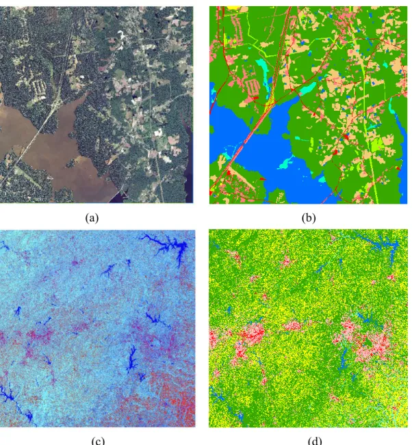
continental U.S., which is administered by the USDA's Farm Service Agency. Each image is rectified and represented as a orthophotograph in three spectral bands, red, green and blue. The experimental area is located in Northeast of Durham County, North Carolina (Figure 1(a)). Considering the availability of image gallery, proposed NAIP image slices were observed on May 31, 2012, to hold the same leaf-on season and nearest observation date compared to utilized Landsat images. In this, the highest degree of similarity was obtained for land cover and plant phenology conditions between two datasets to minimize the bias across datasets. The size of the chosen image is equal to a 6720 pixel width square, corresponding to 45.158 km2 . The chosen area is a complex rural region mixed with forests, low density developed area, open water, cropland, wetland and pasture. Existing research found that the rural setting with complicated landscape decreases classification accuracy compared to urban scenarios (Smith, et al. 2002; Awuah, et al. 2018). Moreover, compared to former rural classification work focused on cropland, the experimental region in Southeast U.S. has moderate coverage of open water and residential area, together with wetland and forest. Former DL land cover classification work focused on very high resolution images in high density urban area (Huang, et al. 2018). There are very limited research that focuses on rural land cover mapping, let alone spatially exhaustive multiple categories classification. Thus the experiment is very innovative and highly valuable for future application of DL for land-cover/land-use classification.
satellite was launched in 1984 (Hansen & Loveland, 2012). The experimental image is located at path 16 and row 35 in Landsat tiling coordinates system, which covers entire central North Carolina region and part of south Virginia (Figure 1(c)). To match with the observation year of NLCD 2011 layer and the leaf-on season of NAIP images, a cloud-free image was captured on May 25, 2011. The proposed image with 7 original spectral bands is preprocessed through Kauth-Thomas (KT) transformation (Kauth & Thomas, 1976; Crist & Cicone, 1984). This transformation is similar to principal components analysis that transforms each band of image into a new coordinate system with a new set of orthogonal axes, however, its transformation coefficients are preset. The first components of KT transformation are generally referred to “brightness”, “greenness”, and “wetness”, respectively, containing nearly all the information in the original 6 bands. The remaining components of KT transformation are often abandoned due to lack of information. As a result, the data volume is reduced and spectral features for land cover classification is preserved To keep the similar volume of training sample size compared to VHR scenarios, the size of the image is set as a 5800 pixel width square, corresponding to 30,276 km2. This region is complicated rural and urban mix, which provides an excellent setting to fully evaluate multi-class classification ability for proposed DL networks. It is important to note that the classifications here in both VHR and medium scenarios are one-time and scene-specific application where training sample and validation sets are chosen in the same image. Thus there is no need to conduct atmospheric correction for images (Song et al. 2001).
has outstanding contextual feature extraction ability similar classes are merged for larger input training patches with more contextual features. The original NLCD 2011 scheme is reclassified based on local land cover characteristics into 8 classes (Table 1), including open water, low density developed, high density developed, barren land, forest & scrub, grassland, cropland, and wetland. Meanwhile, the reference land-cover/land-use map for NAIP images is developed based on visual interpretation (Figure 1 (b)). Since the study area for VHR scenarios do not have barren land coverage, thus proposed classification scheme only holds 7 categories. Previous studies (Dannenberg, et al. 2016; Wickham, et al. 2013) recognized the difficulty in classifying low density urban (class 21 in Table 1). Those pixel groups consist of rural residential site that have an independent house in the center and are surrounded by grassland. Thus they hold similar spectral features with grass-dominated categories and are easily mis-classified through
(a) (b)
(c) (d)
Figure 11 . The materials of the study. (a) The NAIP image with 1-meter resolution for study area. (b) The manually delineated 7-class land cover map based on NAIP image. (c) The Tasseled Cap transformation of Landsat image with 30-meter resolution for study area. (d) Reclassified 8-class NLCD 2011 layer corresponding to proposed Landsat image.
1Legend: open water (blue); low density developed (pink); high density developed (red); forest (dark green);
Table 1. Reclassification lookup table conceived from NLCD 2011 scheme
Class Definition NLCD
class
Definition
1 Open Water 11 Open Water
2 Low density developed 21 22
Developed, Open Space Developed, Low Intensity 3 High density developed 23
24
Developed, Medium Intensity Developed High Intensity
4 Barren Land 31 Barren Land
5 Forestry/ Scrub 41
42 43 52
Deciduous Forest Evergreen Forest Mixed Forest Scrub/Shrub
6 Grassland 71 Grassland/Herbaceous
7 Cropland 81
82
Pasture/Hay Cultivated Crops
8 Wetland 90
95
Woody Wetlands
Emergent Herbaceous Wetlands
2.2 Training data generation
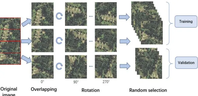
In this subsection, the generation of training and validation datasets are introduced for all experimental scenarios (Figure 2). DL networks training process needs plenty of training image patches with fixed size in each dimension for forward and back propagation of weights.
Compared to popular benchmarks like ImageNet (Deng et al. 2009) that consists of more than a million independent and different-sized image patches, wall-to-wall pixel-level land cover classification datasets only provide continuous single images. In this, it was important to
bands, each input training patch is a 3×224×224 tensor for all scenarios. As Figure 2 shows, mosaic tiling extraction is conducted towards the original image. Taking 1-meter scenario as an example, 6720×6720 pixel size original image will be divided into 900 mosaic patches.
Figure 2. The patch extraction and augmentation of training and validation datasets.
2.3 Deep residual fully convolutional networks (DRFCN)
In this section, a plain introduction of deep convolution neural networks for image categorization is provided. This part is important since proposed framework is built on those basic modules. Then, the definitions of fully convolutional networks (FCN) and deep residual networks (ResNet) are provided, which are core strategies in this thesis. Finally, to address dense-pixel multiclass classification work, changeable deep residual fully convolutional networks (DRFCN) are created and adapted to all experimental scenarios.
2.3.1 Convolutional neural networks (CNNs)
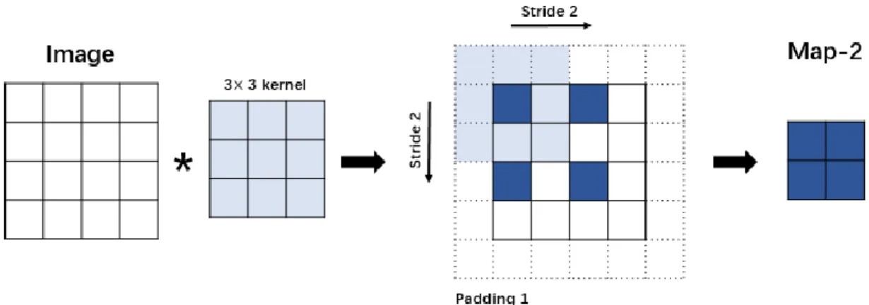
classification work, the first layer is the input remote sensing image patches as 3D tensors (3×224×224), which contains 3 channels of 2D images (224×224). During the feedforward process of the first convolutional layer, convolutional kernels with size of 3×k×k pixels will extract contextual features with stride s covering each 2D image. It sums values up among channels into a feature map with size of (224 − 𝑘) 𝑠⁄ + 1. Figure 2 gives an explicit visual illustration of convolutional processing with default padding. Here the stride is defined as the distance between two continuous kernels during convolution process, and padding is defined as the width added to edges of original images before convolution. If stride s is larger than 1, the size of feature map will reduce with factor of s, which is similar as down-sampling. To extract various features, researchers usually propose m multiple different convolutional kernels towards a single input image. Thus, we obtain m different feature maps in the second layer of the CNNs. Equation 2.1 illustrates how to calculate each pixel value 𝑋𝑖𝑗𝑛 at position of ith row and jth column of a feature map in n+1th layer of the networks, assuming nth layer has m channels of feature maps:
𝑋𝑖𝑗𝑛+1 = ∑ 𝑊𝑘𝑛
𝑚
∗ 𝑋𝑟𝑐𝑛 + 𝑏𝑛 , 𝑤ℎ𝑒𝑟𝑒 𝑟, 𝑐 ∈ [𝑖, 𝑗 −𝑘
2, 𝑖, 𝑗 + 𝑘
2] (2.1)
convolutional layer translates invariance features through feedforwards processes. And a typical convolutional structure can fit 2D images with any sizes and amount. This multiple input and output convolution processes repeat through each feedforward process from low to high layer of the networks, in order to extract contextual features from shadow to deep level.
In terms of land cover image inputs, the first convolutional layers may extract simple features like edges and corners, while the next layer may extract more complex features like edge directions or corner distributions (Luo, et al. 2018). Since convolutional kernels across a
particular feature map share weights, the volume of parameters is extremely reduced compared to conventional neural networks or fully connected layer with similar structure. With the usage of GPU which is designed for efficient convolutional calculation, a CNNs can be trained and
implemented with reasonable time cost.
Figure 3. The illustration of a convolutional processing. The input image size is 4×4, kernel size
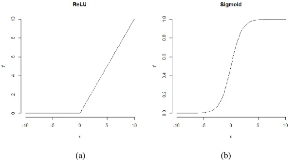
then deliver those features into next feature maps. In other words, it rarefies the neural networks for faster convergence. Commonly, Rectified Linear Unit (ReLU) function 𝑓(𝑥) = 𝑚𝑎𝑥 (𝑥, 0) is utilized for CNNs to prevent vanishing gradient problem, instead of conventional activation functions like sigmoid function (Figure 4). For output value near 0 or 1 in sigmoid function, corresponding residual gradients through back propagation will be close to 0. Thus, gradients will vanish from deep to shadow structures, which makes no significant parameter updates in low layers. While ReLU function keeps linear activation for input value above 0. Gradients for weights updating from higher layers will be effectively transmitted to low layers. The simple threshold arithmetic function will also reduce calculation burden through feedforwards processes compared to exponential calculation from sigmoid.
(a) (b)
Figure 4. Visual illustrations of nonlinear functions. (a) The ReLU function. (b) The Sigmoid function.
pooling layers are promoted following convolutional layers to unify and summarize features. It is usually defined as local maximum or average function, acting as a selection or smooth filter for each feature map. With similar concept of convolutional layers, maximum or average pooling process is illustrated through Equation 2.2:
𝑋𝑖𝑗𝑛+1 = 𝑚𝑎𝑥 𝑜𝑟 𝑎𝑣𝑔{ 𝑋𝑟𝑐𝑛} , 𝑤ℎ𝑒𝑟𝑒 𝑟, 𝑐 ∈ [𝑖, 𝑗 −
𝑘 2, 𝑖, 𝑗 +
𝑘
2] (2.2)
where pooled pixel value is decided by group characteristics from neighboring pixels in the last layer. Unlike convolutional layer, pooling layer does not provide multiple input or multiple output mechanism, and the channel number is fixed. Pooling function generally implements with a pre-defined stride which is larger than 1, in order to down-sample the convoluted feature maps. This down-sampling process aims to increase the so-called receptive field in higher layers, where a path-connected region of original image corresponding to a pixel in higher layers. For instance, the receptive field of a heat map pixel after a 2-stride, 3×3 kernel pooling layer is a 3×3 region (Figure 2). The stride in convolutional layer has similar effect. This process makes feature maps more robust towards noise and heterogeneous variations within an object. Further, it will
dramatically reduce the number of parameters transmitted to next convolutional layer. It will also accelerate the training process and reduce the burden of device runtime memory.
Generally, CNNs is a composite of aforementioned convolutional layers, including convolution, activation, and pooling layers. In some widely used CNNs like AlexNet (Krizhevsky & Hinton, 2012), several fully connected layers connect the end of stacked
feature maps and a 1D feature vector with the length of possible class number. Each element of the vector indicates the probability of assigning the input image to corresponding class. This layer usually performs with softmax function to transform and summarize features from feature maps into a probability distribution or categorization score. Finally, a proposed classifier will be trained by those deep feature vectors for final class decision. Unlike former convolutional layers, fully connected layers has considerable parameters. Its increasing volume is directly proportional to expanding size of feature maps. The parameter volume will significantly increase under large image input or multiple classification situations. Moreover, overfitting phenomena may be amplified by large amount of direct connections. This layer is great for summarizing and
representing features for categorization, but all spatial details will be lost through this layer, since final feature vector is 1D. The proposed method will not utilize this layer.
The training of a general CNNs can be considered as an optimization of a non-linear function from images to categorized labels. This optimization problem should have a loss function L, where all weights and biases in the networks will be updated through each ergodic iteration, in order to minimize L. Loss function L is proposed to quantitatively evaluate the performance of a CNNs, and to simulate how the predicted probability distribution matches the ground truth labels. It also provides a quantified criterion for back propagation during training. For this thesis, I utilize a common multi-classification loss function, cross entropy loss (Equation 2.3) as L:
𝐿(𝑥, 𝑝) = − ∑ 𝑥𝑖𝑙𝑜𝑔 𝑝𝑖 𝑖
where x is the ground truth probability and p is the predicted probability for all categories indexed as i. This function is proposed to evaluate the distance between targeted probability distribution and predicted probability distribution. Through the backpropagation process,
derivative of L is calculated to update parameters of aforementioned convolutional layers with a learning rate 𝜆 as Equation 2.4 shows:
𝜔𝑖+1 = 𝜔𝑖 + 𝜆 𝜕𝐿
𝜕𝜔𝑖 (2.4)
where i indicates the number of iteration times. For weights in low layers, chain rule is used to compute the derivatives through higher layer. Thus the optimization problem is solved by gradient descent strategy through above mechanism. When the loss function reaches the minimum optimal value, the networks gets convergence. Thus we finally get the trained CNNs representing a nonlinear function from images to predicted labels.
2.3.2 Fully convolutional networks (FCN)
The FCN for semantic segmentation is first introduced to DL dense pixel classification at 2015 (Long, et al. 2015). As I discuss in Section 2.3.1, general CNNs is only able to answer “what is here?” It loses spatial details by down-sampling and fully connected layers. For wall-to-wall pixel-level land cover classification mission in this study, I need to answer “what and where”, which combines both categorization and spatial localization. Thus FCN is proposed in this paper to solve this combined problem.
represented by Equation 2.5 with kernel size k, and stride s. Here 𝑓𝑘𝑠 can be any layer types, including multiplication of convolution or pooling process, or nonlinearity activation function.
𝑋𝑖𝑗𝑛+1 = 𝑓𝑘𝑠(𝑋𝑠𝑖+𝑟,𝑠𝑗+𝑐𝑛 ) 0 ≤ 𝑟, 𝑐 ≤ 𝑘 (2.5)
Inferentially, for n-stacked multiple layers contain {𝑓𝑘11𝑠1 𝑓 𝑘2𝑠2
2 … 𝑓 𝑘𝑛𝑠𝑛
𝑛 }, the entire networks
can be described as a combined nonlinear filter 𝑔𝑘,𝑠, in Equation 2.6:
𝑔𝑘,𝑠, = 𝑓𝑘 1𝑠1
1 ° 𝑓 𝑘2𝑠2
2 ° … ° 𝑓 𝑘𝑛𝑠𝑛
𝑛 = (𝑓1 ° … ° 𝑓𝑛)
𝑘,𝑠, (2.6)
where ° indicates convolution process, 𝑘, and 𝑠, for the integral filter 𝑔 are decided by a variety of stride s and kernel size k under convolutional transformation rule. Under this strategy, the input and output of 𝑔 is both 3D tensors, where the size of output tensor is determined by the size of input images and layer settings. Compared to CNNs discussed in Section 2.3.1, FCN can train images with any sizes. And we can control the output size of feature maps through layer settings. In this, the last layer of feature maps can be set as pixel-level classification probability prediction, in order to provide end-to-end loss function between output feature maps and ground truth. Here the function is real-valued, and training is targeted to each output pixel through similar backpropagation flow in Section 2.3.1. For easy understanding, FCN synthesizes general convolutional layer processing and provides localized dense-pixel prediction for proposed land cover classification work.
stride and pooling during convolutions. I have discussed that increasing receptive field benefits robustness and representativeness of extracted features for better classification performance. Meanwhile, down-sampling accompanies with receptive field increasing, which makes output feature maps smaller than original images. Here I introduce the deconvolution layer, which is an up-sampling filter acting as backwards convolution with a fractional stride 1/𝑓. The processing of deconvolution is the same as convolutional multiplication but in transposed version. In this, the output size of filter can be expanded. For end-to-end prediction, we may conduct
deconvolution layers with the same up-sampling factor corresponding to down-sampling factor during convolution layers. It is important to recognize that the weights of deconvolution filters can also be obtained during the training iterations, thus a stacked deconvolution layers with nonlinearity activation can represent a nonlinear up-sampling processing and label prediction.
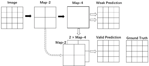
FCN is usually utilized as a technical skill together with general CNNs like VGG for dense-pixel classification work. However, there is inevitable spatial detail loss before
bring better spatial details for further 2-factor deconvolution. This 2-stage deconvolution
provides valid prediction compared to directly 4-factor deconvolution from Map-4. This strategy will bring more useful spatial details for a valid dense-pixel prediction. To be noted, this strategy can be used in any layers of the networks. When the output tensor and shortcut feature maps have different channel numbers, we may propose a 1-stride convolutional layer to change the channel without change size.
Figure 5. The illustration of FCN end-to-end prediction framework. Solid arrows indicate stride 2 convolutional filtering. Hollow solid-outlined arrows indicate deconvolution with factor 1/2. Hollow dash-outlined arrows indicate identity mapping.
2.3.3 Residual networks (ResNet)
the accuracy of networks will get saturated with increasing depth. This problem does not occur from overfitting, and sometimes adding extra layers will even decrease accuracy compared to shadow structure. He et al. (2015) found that training the residual of a nonlinear mapping is much easier than training the original mapping function. In an extreme case that targeted
nonlinear function is identity mapping, a randomly initialized networks is easier to be optimized to zero (residual) rather than to be optimized as an identity mapping.
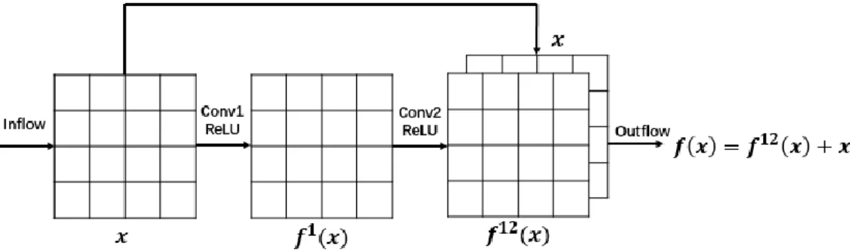
Deep residual learning explicitly changes the targeted mapping 𝑥 → 𝑓(𝑥) of a convolutional layer stack to its residual as 𝑥 → 𝑓(𝑥) − 𝑥. The structure of a basic residual learning block for a given band is showed in Figure 6. Each basic block contains 2 convolutional layers and corresponding nonlinearity ReLU layers. Through identity mapping of inflow x
towards original outflow, targeted function changes from 𝑓(𝑥) to its more trainable residual 𝑓12(𝑥) = 𝑓(𝑥) − 𝑥. It will help fully exploit benefits of deep structure in order to extract and
Figure 6. The illustration of a basic block of residual learning, which contains 2 convolutional layers. Targeted function changes from 𝑓(𝑥) to its residual 𝑓12(𝑥) = 𝑓(𝑥) − 𝑥.
2.3.4 Depth-adaptive DRFCN
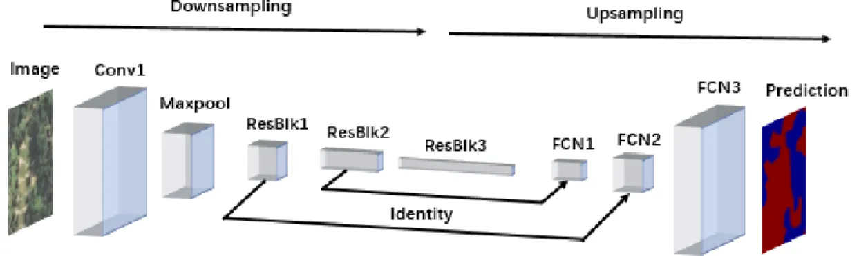
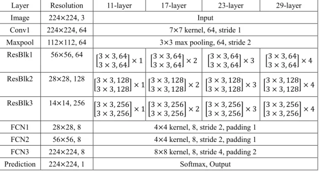
In this paper, I combine deep-featured categorization ability from CNNs, end-to-end dense prediction ability from FCN, and trainability of deep structures from ResNet. This mixed networks is called DRFCN. Figure 7 provides a visual illustration of how the image size and channel change through DRFCN, corresponding networks architecture is showed in Table 2. The input image with size of 3×224×224 will be convoluted by a stacked convolutional (Conv1) layer and maxpooling (Maxpool) layer. It is transformed to feature maps with size of
tensor, where each 8-length vector indicates classification probability towards 8 possible classes. A softmax transformation will be conducted for final end-to-end prediction of each pixel, which is a 1×224×224 output classification result. This DRFCN provides end-to-end pixel-level classification for land cover mapping, and it is adaptive to different depths of networks structures. The networks is easy to be trained with light device requirement.
For experimental scenarios with different levels of classification difficulties, I provide adaptive network structures from 11 layers to 29 layers, to understand the effect of the network structure on classification accuracy. I will implement the same training process for all four types of structures in each experimental scenario. I will further analyze the dynamics of classification accuracy, convergence speed, and memory usage through each networks structure. To be noted, training approaches are implemented with a CPU of Intel i7-7700HK, and a GPU of NVIDIA GTX 1050Ti with only 2 Gbps memory. Because of the limitation of GPU power, the time cost in this paper may be much longer than other researches under similar situation.
Table 2. The architecture of DRFCN in adaptive layer depth. The number after comma indicates channels, the number after times sign for three residual blocks (ResBlk1-3) is indicates stacked basic blocks. Down-sampling is in Maxpooling, ResBlk1, ResBlk2, ResBlk3, with stride of 2 for each. Up-sampling is in FCN1, FCN2, FCN3, with stride of 2, 2, 4, respectively.
Layer Resolution 11-layer 17-layer 23-layer 29-layer
Image 224×224, 3 Input
Conv1 224×224, 64 7×7 kernel, 64, stride 1 Maxpool 112×112, 64 3×3 max pooling, 64, stride 2 ResBlk1 56×56, 64
[3 × 3, 64
3 × 3, 64] × 1 [
3 × 3, 64
3 × 3, 64] × 2 [
3 × 3, 64
3 × 3, 64] × 3 [
3 × 3, 64 3 × 3, 64] × 4
ResBlk2 28×28, 128
[3 × 3, 1283 × 3, 128] × 1 [3 × 3, 1283 × 3, 128] × 2 [3 × 3, 1283 × 3, 128] × 3 [3 × 3, 1283 × 3, 128] × 4
ResBlk3 14×14, 256
[3 × 3, 256 3 × 3, 256] × 1[
3 × 3, 256 3 × 3, 256] × 2 [
3 × 3, 256 3 × 3, 256] × 3 [
3 × 3, 256 3 × 3, 256] × 4
CHAPTER 3: RESULTS
3.1 Training setting
experiment, the batch size is 8, indicating that networks will be modified by the average loss of every 8 input images within a full iteration. It is relatively small compared to existing studies with 64 batch size or more.
3.2 Impacts of spatial resolution and layer structure
This study provides a wall-to-wall accuracy assessment between DRFCN prediction and ground truth dataset among every experiment. This dense-pixel assessment is more robust and credible than random point selection assessment (Ma, et al. 2017). The experiment is multiclass dense-pixel classification work. For assessment of complex spatial resolution and layer structure impacts, several indicators are introduced, including overall accuracy (OA), Kappa coefficient (Kappa), and detailed producer’s accuracy (PA) and user’s accuracy (UA) for every class. The evaluation also includes convergence speed and stability, together with time and memory cost for classification.
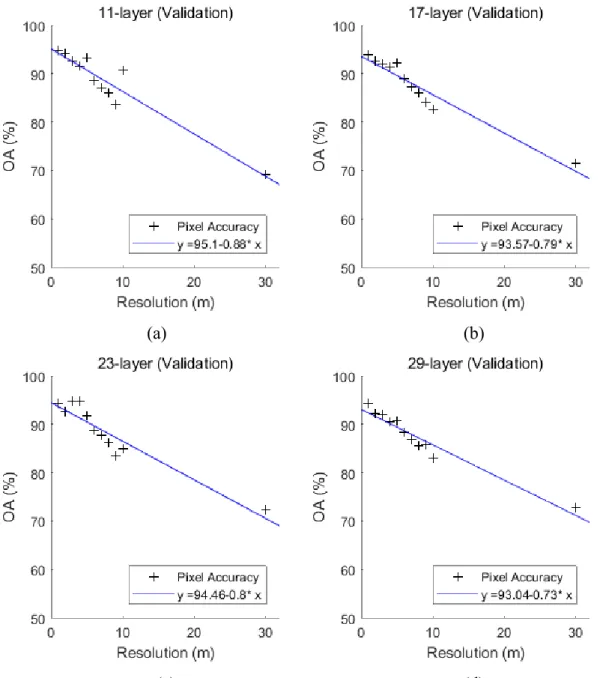
This study evaluates impacts of resolution within fixed network structure, and assesses the impacts of layer structure within a fixed resolution scenario. Two major patterns are
corresponding spatial resolution. Specifically, regression results indicate that degradation rates of OA decrease from 0.88 to 0.73 through 11-layer structure to 29-layer structure. Shadow structure achieves higher OA than deep structure in fine resolution scenarios, but holds lower OA in coarse resolution scenarios. Meanwhile, the scattered points of OA distribute with larger variation in 11-layer structure than that with 29-11-layer structure. Both patterns illustrate that deeper structure is more robust towards resolution degradation in terms of OA. Degradation rate of Kappa has similar pattern with OA. Its value decreases from 0.0135 to 0.0111 through 11-layer structure to 29-layer structure. Shadow structure achieves higher Kappa in fine resolution scenarios, while deep structure outstands coarse resolution.
Furthermore, the study synthesizes the best OA and Kappa performance among 4
be the margin between the utilization of shadow 11-layer structure and intermediate 17/23-layer structures. While 9 meter might be the margin between the utilization of intermediate structures and deep 29-layer structure.
During training iterations, contemporary model parameters are implemented on
validation sets in each iteration. This process is independent to training processes, where OA and training loss based on validation sets are only collected as indicators of model convergence, instead of being utilizing for back-propagation. Among 11 scenarios, 4 representative scenarios (2m, 3m, 9m, 30 m) holding different best-performed networks structures are selected for illustration. In 2-meter scenario (Figure 11 (a)), 11-layer structure holds the fastest convergence and achieve the highest OA. The 17-layer structure holds the second fastest convergence but with less OA than 23-layer, while 29-layer has the slowest convergence and the lowest OA. In terms of training loss within validation set (Figure 11 (b)), all structures have similar decreasing pattern. After learning rate reduction at 500th iteration, the training loss increases slightly, while the training loss for training set continues to decrease. This indicates a certain level of
overfitting. Both OA and training loss curves hold large fluctuations with high learning rate, and curves become stable after the learning rate decays. In 3-meter scenario (Figure 11 (c)),
achieve better OA performance. There is also a slightly lifting pattern for 23-layer and 29-layer structures after learning rate reduction. In the 9-meter scenario (Figure 12 (a-b)), the deep 29-layer outperforms other structures with faster convergence and higher OA, together with lower training loss in the end of training iterations. This indicates that deep structure started from 29-layer fits relatively well for pixel sizes larger than 9x9 meters. This result is verified by a medium 20-meter scenario (Figure 12 (c-d)), where deep 29-layer structure outperforms other shadow structures with faster convergence and higher OA. There is an explicit pattern of overfitting after around 100th iteration, all 4 layer structures’ validation OA decreases and training loss increases till the end of iterations. This indicates our dataset from Landsat may contain correlated spatial and spectral features, which makes DRFCN simulate training set too well and relatively unsatisfied with validation set. All those patterns through training iterations verify the regression results in Figure 8&9, illustrating deeper structures adapt to classification in relatively coarse resolution, and vice versa.
(a) (b)
(c) (d)
(e) (f)
(g) (h)
(a) (b)
(a) (b)
(c) (d)
(a) (b)
(c) (d)
Table 3. DRFCN OA performance rankings and comparison to MLC
1m 2m 3m 4m 5m 6m 7m 8m 9m 10m 30m
MLC 68.74 69.56 68.67 69.55 68.63 69.57 68.67 69.57 68.68 69.56 39.20 DRFCN
Ranking (layer)
1 94.82 (11) 94.18 (11) 94.79 (23) 94.67 (23) 93.19 (11) 88.98 (17) 87.64 (23) 86.12 (23) 85.72 (29) 90.75 (11) 72.66 (29) 2 94.35
(29) 92.72 (23) 92.53 (11) 91.54 (11) 92.10 (17) 88.71 (23) 87.39 (17) 85.97 (17) 84.02 (17) 84.99 (23) 72.31 (23) 3 94.27
(23) 92.54 (17) 91.98 (17) 91.28 (17) 91.84 (23) 88.56 (11) 87.17 (11) 85.94 (11) 83.72 (11) 83.00 (29) 71.39 (17) 4 93.86
(17) 92.12 (29) 91.92 (29) 90.39 (29) 90.63 (29) 88.40 (29) 86.76 (29) 85.59 (29) 83.37 (23) 82.52 (17) 69.12 (11)
Table 4. DRFCN Kappa performance rankings and comparison to MLC
1m 2m 3m 4m 5m 6m 7m 8m 9m 10m 30m
MLC 0.531 0.541 0.532 0.541 0.531 0.541 0.532 0.541 0.532 0.541 0.243 DRFCN
Ranking (layer)
1 0.900 (11) 0.888 (11) 0.904 (23) 0.902 (23) 0.886 (11) 0.786 (17) 0.783 (23) 0.728 (23) 0.729 (29) 0.851 (11) 0.559 (29) 2 0.891
(29) 0.859 (23) 0.865 (11) 0.850 (11) 0.867 (17) 0.782 (23) 0.777 (17) 0.726 (17) 0.694 (17) 0.757 (23) 0.554 (23) 3 0.889
(23) 0.855 (17) 0.855 (17) 0.845 (17) 0.863 (23) 0.777 (11) 0.772 (11) 0.724 (11) 0.689 (11) 0.724 (29) 0.538 (17) 4 0.881
(17) 0.846 (29) 0.853 (29) 0.830 (29) 0.842 (29) 0.775 (29) 0.768 (29) 0.720 (29) 0.679 (23) 0.716 (17) 0.503 (11)
Table 5. The single-patch classification time and parameter volume for all 4 structures DRFCN structures Parameter volume Classification time
11-layer 4.76 MB 0.0058s
17-layer 10.6 MB 0.0077s
23-layer 16.6 MB 0.0094s
29-layer 22.5 MB 0.0111s
3.3 Insights of spatial resolution impacts on DRFCN
structure is not explicit and with random variations, the analysis will focus on spatial resolution impacts. Generally, both PA and UA decrease with increasing spatial resolution. Detailed analysis in Table 6 indicates that each class obtains higher PA than UA except forest and cropland classes. This indicates that pixels of other five classes are misclassified into forest and cropland classes. Those two classes consist of 58% and 11% pixels of the experimental area. Though the percentage difference between PA for those two classes is small, but it counts considerable number of pixels. Due to the criterion of manual sketching for the reference map, some individual forest pixels were classified into other land cover patches like low-density developed, cropland, and grassland (Figure 13 (a,b)). DRFCN currently recognizes those forest pixels, but not classifies them into the classes where they are in the reference map. The mixed spectral features between forest and wetland also contributes to misclassification (Figure 13 (b)). When the large land cover patches contain heterogeneous textures, misclassification also occurs (Figure 13 (c, d)). Also, there is complex misclassification in medium resolution scenario (Figure 13 (l)). Those representative situations are mainly because of spectral confusion and manual sketching criterion, where spectral confusion may be aggravated by increasing spatial resolution.
than common understanding that finer resolution will provide more spatial details for better classification performance. This indicates factors of feature extracting ability and geometric transferability by DRFCN in this study. There are limitations of DRFCN on extracting complex geographic features, and persisting geometric shapes of heterogeneous land cover patches through networks processing.
there are enough fine textures and spectral heterogeneity within those pure forest patches, they are classified properly with minor mistakes (Figure 13 (c)). Through down-sampling, the coverage of water pixels decreases, water pixels are much better recognized (Figure 13 (j)). This lack of feature extraction ability is likely to be the main reason for low classifying accuracy of open water. It also has similar influence to other classes, which may reduce the decreasing rate of classification accuracy.
92.06 (1m) (a)
81.01 (1m) (b)
99.52 (1m) (c)
97.31 (1m) (d)
73.97 (1m) (e)
98.24 (1m) (f)
96.52 (2m) (g)
95.10 (3m) (h)
93.76 (5m) (i)
90.59 (7m) (j)
86.53 (9m) (k)
68.63(30m) (l)
Figure 132. The visualization of representative classification results by best-performed DRFCN from 1-meter to 30-meter resolution. (a-b) Factor of spectral confusion and manual sketch criterion. (c-e) Factor of feature extraction ability. (f-l) Factor of geometric transferability.
21st row: original image; 2nd row: ground truth; 3rd row: DRFCN prediction; numbers and length values
Table 6a. The PA and UA for 1-4m scenarios. The best-performed structure is in bold. Class Resolution Open water L-dens develop H-dens develop Forest, shrub Grass, pasture Crop-land
Wetland Barren land 1m
11-ly UA PA 97.82 82.05 90.17 87.73 92.17 81.68 96.17 99.01 90.57 79.77 90.89 92.59 94.66 59.01 NA 17-ly UA PA 97.61 81.88 91.06 86.28 93.69 81.51 94.68 98.95 87.35 72.74 90.88 88.22 91.31 56.37 23-ly UA PA 97.03 81.41 93.16 87.55 94.06 83.35 94.94 99.12 88.38 74.74 91.42 88.98 92.25 58.51 29-ly UA PA 97.33 84.78 93.26 88.24 94.09 84.25 94.71 99.13 88.33 69.22 92.96 87.92 90.27 62.57 2m
11-ly UA PA 97.25 79.09 90.08 85.88 92.91 84.55 94.24 99.16 93.70 71.15 94.25 91.99 98.18 76.86 NA 17-ly UA PA 96.67 63.96 89.87 83.52 92.69 85.69 92.29 99.03 91.73 70.73 93.24 90.66 96.75 70.93 23-ly UA PA 96.81 66.93 89.89 83.32 91.94 87.46 92.54 98.87 92.27 71.54 93.07 91.11 97.24 70.28 29-ly UA PA 95.72 61.49 88.83 83.01 91.87 87.85 91.72 98.90 91.05 69.65 94.62 91.39 96.22 63.89 3m
11-ly UA PA 97.95 66.72 89.14 82.45 85.45 79.61 92.88 98.86 93.07 88.52 90.41 93.69 95.30 77.18 NA 17-ly UA PA 97.00 62.09 89.29 83.65 88.21 78.16 92.85 98.68 93.55 87.59 88.15 94.35 92.59 71.78 23-ly UA PA 96.24 83.73 90.04 85.54 87.44 79.62 96.49 98.61 91.95 85.69 90.30 93.92 92.19 78.23 29-ly UA PA 96.99 62.55 88.93 84.57 88.48 79.60 92.02 98.53 91.91 83.07 91.18 94.43 87.24 69.57 4m
Table 6b. The PA and UA for 5-8 m scenarios. The best-performed structure is in bold. Class Resolution Open water L-dens develop H-dens develop Forest, shrub Grass, pasture Crop-land
Wetland Barren land 5m
11-ly UA PA 98.29 93.60 91.41 79.66 76.35 65.82 92.74 98.77 94.96 82.31 94.85 88.78 86.92 58.57 17-ly UA PA 97.37 82.95 90.75 82.32 81.20 61.68 91.76 98.73 93.72 81.97 92.27 88.76 82.20 58.44 23-ly UA PA 97.39 82.28 90.03 79.89 81.41 64.38 92.20 98.73 92.82 79.00 88.48 89.46 91.53 61.25 29-ly UA PA 97.03 73.31 89.98 80.23 82.43 63.41 90.84 98.64 91.94 77.27 86.68 89.39 91.17 53.91 6m
11-ly UA PA 89.34 93.74 86.68 56.79 78.91 40.62 89.98 97.79 91.09 71.66 82.55 90.82 95.20 87.16 NA 17-ly UA PA 86.19 94.66 84.68 58.80 81.69 45.16 90.62 97.91 92.60 71.48 83.09 90.50 97.74 79.95 23-ly UA PA 86.79 95.03 86.18 57.77 79.57 40.64 90.71 97.51 88.21 75.93 80.71 91.48 98.39 83.51 29-ly UA PA 89.12 92.80 83.59 57.00 79.38 39.98 90.54 97.62 90.14 72.21 79.96 91.38 96.35 78.98 7m
11-ly UA PA 97.16 95.23 67.17 28.47 40.69 24.92 88.69 97.33 82.00 29.24 64.16 74.58 92.89 68.63 NA 17-ly UA PA 97.32 95.39 68.10 31.75 52.50 27.59 89.11 97.07 78.48 31.54 63.06 76.23 91.67 61.75 23-ly UA PA 96.65 95.75 70.47 33.77 55.58 27.37 89.78 96.79 80.78 30.05 62.27 78.24 89.58 67.31 29-ly UA PA 96.34 94.47 68.79 29.78 50.53 28.63 89.62 96.19 80.82 28.97 58.24 79.68 90.82 62.61 8m
Table 6c. The PA and UA for 9-10m, 30 m scenario. The best-performed structure is in bold. Class Resolution Open water L-dens develop H-dens develop Forest, shrub Grass, pasture Crop-land
Wetland Barren land 9m
11-ly UA PA 74.60 64.15 69.10 55.07 48.09 22.76 83.66 97.53 84.65 40.91 91.50 74.12 97.51 35.90 NA 17-ly UA PA 66.51 60.79 70.20 52.33 47.84 18.71 84.15 98.00 86.65 40.70 91.09 76.32 95.83 32.89 23-ly UA PA 64.93 54.48 73.95 53.01 49.76 16.59 83.40 98.53 81.77 36.78 89.19 73.68 99.34 27.68 29-ly UA PA 69.63 61.82 76.24 61.68 59.55 28.18 85.40 98.45 89.71 44.62 93.02 77.95 95.04 34.47
10m 11-ly UA PA 98.80 92.12 80.91 55.32 70.15 37.53 87.63 97.60 85.85 71.55 81.25 85.41 91.09 82.83 NA 17-ly UA PA 98.80 69.72 75.23 56.74 68.40 36.22 77.09 97.55 84.35 72.37 72.06 86.56 83.83 80.87 23-ly UA PA 98.51 77.26 76.65 58.30 68.86 41.17 80.46 97.21 89.20 70.86 69.09 83.92 92.00 69.56 29-ly UA PA 98.49 72.47 72.76 57.73 68.83 40.78 77.71 97.16 91.37 66.55 71.80 82.08 87.02 69.65 30m
CHAPTER 4: DISCUSSIONS
4.1 Illustrations of DRFCN
This paper proposes DRFCN as classifier for wall-to-wall land cover land cover classification work. It is capable to handle different spatial resolution scenarios and various networks structure with different layer depths. DRFCN innovatively combines advantages of deep feature extraction, wall-to-wall prediction, and depth-adaptive structures from CNNs (Huang et al. 2018; Hu et al. 2015), FCN (Long, et al. 2015; Maggiori, et al. 2017), and ResNet (He, at al. 2015), respectively. Compared to existing studies on patch-based very deep CNNs on land cover categorization (Mahdianpari, et al. 2018; Huang, et al. 2018; Mnih, 2013), DRFCN does not experience discontinuities among adjacent patches and provides pixel-level prediction without other auxiliary GIS data. Compared to moving-patch algorithm which predicts centers of sliding patches to provide pixel-level prediction (Sermanet et al. 2013), DRFCN holds faster classification speed and lighter memory cost. In summary, DRFCN is a remote-sensing
adaptation of DCNNs from different computer vision tasks, in order to conduct pixel-level land cover mapping. It is able to provide satisfactory OA and Kappa of wall-to-wall land cover classification from 1-meter to 30-meter resolution.
of residual learning blocks. This paper provides a coherent guidance for the choice of spatial resolution and corresponding structure design of DRFCN. Though the results already illustrate explicit patterns, the range of resolution and network structure is still limited within 1 meter to 30 meter, and 11 to 29 layers, respectively. With possible future works aiming to fill the resolution gap (10m - 30m) and extend resolution range (>30m), and to implement deeper networks structures with more iterations, proposed results may provide a boundary point of image resolution between the utilization of conventional machine learning algorithms and DCNNs. Since various DCNNs share similar constituent layers, insights of influences between spatial resolution, networks structure, and networks performance in this paper will enlighten networks design of new DCNNs in broader geographic researches. Moreover, the training processes of DRFCN cost reasonable time and light device burden, addressing the device limitation hindering expansion of DCNNs utilizations in large-scale geographic researches. In summary, proposed DRFCN provides possibilities of further discoveries on resolution impacts of DCNNs. And it will also aspire the utilizations of DCNNs in broader geographic researches. 4.2 Comparison to Maximum Likelihood Classification (MLC)
down-sampling within the range of 1 to 10 meter. It is understandable by its classification theory that only the spectral information from each pixel is utilized. Within high resolution range (1m-10m), since the spectral confusion is not serious enough to significantly influence pixel-level spectral distribution, the classification results are stable. Moreover, down-sampling process actually smoothens some heterogeneous spectral features within complex class patches. It will slightly reduce the salt and pepper noise in final classification results, thus there is an
inconspicuous increase of OA and Kappa performances through down-sampling. Existing studies of spatial resolution impacts on conventional classification algorithms based on medium
resolution images (Awuah, 2018; Fisher, et al. 2017) found OA and Kappa decrease with increasing pixel size. But this decreasing pattern is missing in VHR scenarios of this study. The possible reason is the different resolution of satellite image dataset with different level of spectral mixing. In this study, there is a sharp cliff between performances in 10-meter and 30-meter scenarios, where OA in 30-meter resolution is considerably low as 39.2%. This may result from lack of sampling, as well as simple classifier, and cross-errors between prediction and NLCD data. Dannenberg (et al. 2018) was able to reach more than 80% OA with NLCCD with the Random Forest classifier. In this case, 29-layer DRFCN leads to lower OA, but it is still
4.3 Full-training strategy
During the practical training of CNNs, apart from networks structure and spatial
resolution, weights initialization, optimization strategy, and setting of hyper-parameters will also significantly influence the convergence and accuracy of proposed networks. Experiments of DRFCN do not utilize fine-tuning procedure which directly starts from pre-trained parameter sets from well-known existing studies. Two reasons are highlighted: (1) remote sensing images, especially with heterogeneous spatial settings, have random shapes and textures. Extracting those complex spatial and spectral features is totally different from the work of extracting features from well-specified image benchmarks like ImageNet (Russakovsky et al. 2015). Pre-trained networks has little possibility to benefit fast convergence and high accuracy in different experimental scenarios in this study. (2) DRFCN is similar but not holding the same structures with any other networks, including VGG, FCN, and ResNet. There are four adaptive structures for DRFCN from 11 to 29 layers. Even borrowing part of parameters to relevant structures, the contribution of this partial fine-tuning process is questionable and hard to be analyzed.
(Kingma & Ba, 2014). This method is adaptive with hyper-parameters, learning rate, and is robust towards local minimum. Learning rate is the only pre-defined hyper-parameter, and networks convergence is not sensitive to its value. Adam optimizer provides stable convergence in middle and late training stages compared to well-known stochastic gradient descent (SGD) in my experiments.
4.4 Limitations
There are several variations concentrated on 5-meter and 10-meter resolution scenarios, which has relatively high accuracy compared to finer resolution scenarios. Those biases are also observed in OA and Kappa curve in Figure 8&9. The most possible reason is the lack of
segmented patches after down-sampling makes the random selection of validation set hold considerable uncertainty. The data augmentation process will also help validation sets overlapped with training sets with different clips after 5-meter down-sampling. Thus some selected
CHAPTER 5: CONCLUSIONS
This paper provides a depth-adaptive deep networks DRFCN for dense-pixel land cover classification. The DRFCN is capable to classify images in a range of spatial resolutions by different networks structures. The performance of DRFCN achieves satisfactory OA and Kappa through VHR to medium resolution, with reasonable time cost and light device burden. The complex impacts of spatial resolution and networks structure are analyzed and synthesized to three empirical understandings: (1) DRFCN performs better than MLC within 1-meter to 10-meter resolution scenarios with at least 85% overall accuracy. It is also competitive compared to random forest in medium resolution. (2) Generally, DRFCN performance negatively relates to increasing pixel size; (3) Shadow DRFCN is more sensitive to spatial resolution dynamics than deep DRFCN. The margins between utilization of shadow 11-layer structure, intermediate 17/23-layer structure, and deep 29-17/23-layer structure are around 3 meter and 9 meter respectively.
REFERENCES
Awuah, T. K. (2018). Effects of spatial resolution, land-cover heterogeneity and different classification methods on accuracy of land-cover mapping.
Awuah, K. T., Nölke, N., Freudenberg, M., Diwakara, B. N., Tewari, V. P., & Kleinn, C. (2018). Spatial resolution and landscape structure along an urban-rural gradient: Do they relate to remote sensing classification accuracy?–A case study in the megacity of Bengaluru, India. Remote Sensing Applications: Society and Environment, 12, 89-98.
Ammour, N., Alhichri, H., Bazi, Y., Benjdira, B., Alajlan, N., & Zuair, M. (2017). Deep learning approach for car detection in UAV imagery. Remote Sensing, 9(4), 312.
Connors, C., & Vatsavai, R. R. (2017, July). Semi-supervised deep generative models for change detection in very high resolution imagery. In 2017 IEEE International Geoscience and
Remote Sensing Symposium (IGARSS)(pp. 1063-1066). IEEE.
Chen, Y., Song, X., Wang, S., Huang, J., & Mansaray, L. R. (2016). Impacts of spatial heterogeneity on crop area mapping in Canada using MODIS data. ISPRS Journal of
Photogrammetry and Remote Sensing, 119, 451-461.
Crist, E.P. and Cicone, R.C., 1984, A physically based transformation of Thematic Mapper data—The TM Tasseled Cap, IEEE Transactions on Geosciences and Remote Sensing, GE-22: 256–263.
Dannenberg, M. P., Song, C., & Hakkenberg, C. R. (2018). A Long-Term, Consistent Land Cover History of the Southeastern United States. Photogrammetric Engineering & Remote
Sensing, 84(9), 559-568.
Dannenberg, M., Hakkenberg, C., & Song, C. (2016). Consistent classification of Landsat time series with an improved automatic adaptive signature generalization algorithm. Remote
Sensing, 8(8), 691.
Dumoulin, V., & Visin, F. (2016). A guide to convolution arithmetic for deep learning. arXiv
preprint arXiv:1603.07285.
Dodge, S., & Karam, L. (2016, June). Understanding how image quality affects deep neural networks. In 2016 eighth international conference on quality of multimedia experience
(QoMEX) (pp. 1-6). IEEE.
Deng, J., Dong, W., Socher, R., Li, L. J., Li, K., & Fei-Fei, L. (2009, June). Imagenet: A large-scale hierarchical image database. In 2009 IEEE conference on computer vision and pattern
Everingham, M., Van Gool, L., Williams, C. K., Winn, J., & Zisserman, A. (2010). The pascal visual object classes (voc) challenge. International journal of computer vision, 88(2), 303-338.
Fisher, J. R., Acosta, E. A., Dennedy‐Frank, P. J., Kroeger, T., & Boucher, T. M. (2018). Impact of satellite imagery spatial resolution on land use classification accuracy and modeled water quality. Remote Sensing in Ecology and Conservation, 4(2), 137-149.
Girshick, R., Donahue, J., Darrell, T., & Malik, J. (2014). Rich feature hierarchies for accurate object detection and semantic segmentation. In Proceedings of the IEEE conference on
computer vision and pattern recognition (pp. 580-587).
Gislason, P. O., Benediktsson, J. A., & Sveinsson, J. R. (2006). Random forests for land cover classification. Pattern Recognition Letters, 27(4), 294-300.
Huang, B., Zhao, B., & Song, Y. (2018). Urban land-use mapping using a deep convolutional neural network with high spatial resolution multispectral remote sensing imagery. Remote
Sensing of Environment, 214, 73-86.
Hamida, A. B., Benoit, A., Lambert, P., Klein, L., Amar, C. B., Audebert, N., & Lefèvre, S. (2017, July). Deep learning for semantic segmentation of remote sensing images with rich spectral content. In 2017 IEEE International Geoscience and Remote Sensing Symposium
(IGARSS) (pp. 2569-2572). IEEE.
He, K., Zhang, X., Ren, S., & Sun, J. (2016). Deep residual learning for image recognition.
In Proceedings of the IEEE conference on computer vision and pattern recognition (pp.
770-778).
He, K., Zhang, X., Ren, S., & Sun, J. (2015). Delving deep into rectifiers: Surpassing human-level performance on imagenet classification. In Proceedings of the IEEE international
conference on computer vision (pp. 1026-1034).
Hu, F., Xia, G. S., Hu, J., & Zhang, L. (2015). Transferring deep convolutional neural networks for the scene classification of high-resolution remote sensing imagery. Remote
Sensing, 7(11), 14680-14707.
Homer, C., Dewitz, J., Yang, L., Jin, S., Danielson, P., Xian, G., ... & Megown, K. (2015). Completion of the 2011 National Land Cover Database for the conterminous United States– representing a decade of land cover change information. Photogrammetric Engineering &
Remote Sensing, 81(5), 345-354.
Huang, C., Davis, L. S., & Townshend, J. R. G. (2002). An assessment of support vector
machines for land cover classification. International Journal of remote sensing, 23(4), 725-749.
Kussul, N., Lavreniuk, M., Skakun, S., & Shelestov, A. (2017). Deep learning classification of land cover and crop types using remote sensing data. IEEE Geoscience and Remote Sensing
Letters, 14(5), 778-782.
Kingma, D. P., & Ba, J. (2014). Adam: A method for stochastic optimization. arXiv preprint
arXiv:1412.6980.
Krizhevsky, A., Sutskever, I., & Hinton, G. E. (2012). Imagenet classification with deep
convolutional neural networks. In Advances in neural information processing systems (pp. 1097-1105).
Kluckner, S., Mauthner, T., Roth, P. M., & Bischof, H. (2009, September). Semantic
classification in aerial imagery by integrating appearance and height information. In Asian
Conference on Computer Vision (pp. 477-488). Springer, Berlin, Heidelberg.
Kurnaz, M. N., Dokur, Z., & Ölmez, T. (2005). Segmentation of remote-sensing images by incremental neural network. Pattern recognition letters, 26(8), 1096-1104.
Kauth, R. J., & Thomas, G. S. (1976, January). The tasselled cap--a graphic description of the spectral-temporal development of agricultural crops as seen by Landsat. In LARS
Symposia (p. 159).
Luo, C., Huang, H., Wang, Y., & Wang, S. (2018). Utilization of deep convolutional neural networks for remote sensing scenes classification. In Advanced Remote Sensing Technology
for Coastal Environment, Disasters, and Infrastructure. IntechOpen.
Li, Y., Zhang, H., & Shen, Q. (2017). Spectral–spatial classification of hyperspectral imagery with 3D convolutional neural network. Remote Sensing, 9(1), 67.
Liu, Q., Hang, R., Song, H., & Li, Z. (2016). Learning multi-scale deep features for high-resolution satellite image classification. arXiv preprint arXiv:1611.03591.
Long, J., Shelhamer, E., & Darrell, T. (2015). Fully convolutional networks for semantic segmentation. In Proceedings of the IEEE conference on computer vision and pattern
recognition (pp. 3431-3440).
LeCun, Y. & Cortes, C. (2010). MNIST handwritten digit database.
Mnih, V. (2013). Machine learning for aerial image labeling. University of Toronto (Canada).
Mahdianpari, M., Salehi, B., Rezaee, M., Mohammadimanesh, F., & Zhang, Y. (2018). Very deep convolutional neural networks for complex land cover mapping using multispectral remote sensing imagery. Remote Sensing, 10(7), 1119.
Maggiori, E., Tarabalka, Y., Charpiat, G., & Alliez, P. (2017). Convolutional neural networks for large-scale remote-sensing image classification. IEEE Transactions on Geoscience and
Remote Sensing, 55(2), 645-657.
Ma, L., Li, M., Ma, X., Cheng, L., Du, P., & Liu, Y. (2017). A review of supervised object-based land-cover image classification. ISPRS Journal of Photogrammetry and Remote
Sensing, 130, 277-293.
Marmanis, D., Datcu, M., Esch, T., & Stilla, U. (2016). Deep learning earth observation
classification using ImageNet pretrained networks. IEEE Geoscience and Remote Sensing
Letters, 13(1), 105-109.
Mishra, V. N., Prasad, R., Kumar, P., Gupta, D. K., Dikshit, P. K. S., Dwivedi, S. B., & Ohri, A. (2015, December). Evaluating the effects of spatial resolution on land use and land cover classification accuracy. In 2015 International Conference on Microwave, Optical and
Communication Engineering (ICMOCE) (pp. 208-211). IEEE.
Mora, B., Tsendbazar, N. E., Herold, M., & Arino, O. (2014). Global land cover mapping: Current status and future trends. In Land Use and Land Cover Mapping in Europe(pp. 11-30). Springer, Dordrecht.
Midhun, M. E., Nair, S. R., Prabhakar, V. T., & Kumar, S. S. (2014, October). Deep model for classification of hyperspectral image using restricted boltzmann machine. In Proceedings of
the 2014 international conference on interdisciplinary advances in applied computing (p.
35). ACM.
Mnih, V., & Hinton, G. E. (2012). Learning to label aerial images from noisy data.
In Proceedings of the 29th International conference on machine learning (ICML-12)(pp.
567-574).
Nguyen, T. T., Kluckner, S., Bischof, H., & Leberl, F. (2010). Aerial photo building classification
by stacking appearance and elevation measurements. na.
Russakovsky, O., Deng, J., Su, H., Krause, J., Satheesh, S., Ma, S., ... & Berg, A. C. (2015). Imagenet large scale visual recognition challenge. International journal of computer