HIGH RESOLUTION AIR QUALITY MODELING FOR IMPROVED 1
CHARACTERIZATION OF EXPOSURES AND HEALTH RISK TO TRAFFIC-RELATED 2
AIR POLLUTANTS (TRAPS) IN URBAN AREAS 3
Shih Ying Chang 4
A dissertation submitted to the faculty at the University of North Carolina at Chapel Hill in 5
partial fulfillment of the requirements for the degree of Doctor of Philosophy in the Department 6
of Environmental Sciences and Engineering in the Gillings School of Global Public Health. 7
Chapel Hill 8
2016 9
Approved by: 10
Saravanan Arunachalam 11
William Vizuete 12
Vlad Isakov 13
Marc Serre 14
1 2 3 4 5 6 7 8 9 10 11 12 13 14 15 16 17 18 19 20 21 22 23 24 25 26 27 28 29 30 31 32 33 34 35 36 37 38
© 2016 39
Shih Ying Chang 40
ALL RIGHTS RESERVED 41
1
ABSTRACT 2
3
Shih Ying Chang: High Resolution Air Quality Modeling for Improved Characterization of 4
Exposures and Health Risk to Traffic-Related Air Pollutants (TRAPs) in Urban Area 5
(Under the direction of Saravanan Arunachalam and William Vizuete) 6
7
Exposure to traffic-related air pollutants in health studies is often obtained from air 8
quality models at a relatively coarse spatial resolution that is unable to capture concentration 9
hotspots near roadways thus has the potential to underestimate the risk. The goal of this work is 10
to improve the characterization of exposure and health risk to traffic-related air pollutants. The 11
hypothesis is that dispersion models can reduce the error for large-scale exposure and risk 12
assessment because of the capability for fine-resolution modeling. This overall hypothesis was 13
verified by the following 3 studies. 14
The first study describes the development of a modeling framework that combined space- 15
time kriging and Gaussian dispersion to inform exposure estimates for traffic-related air 16
pollutants with a high spatial resolution. This framework reduces CPU-time by 88-fold by 17
reducing the required meteorological data, while retaining the accuracy of exposure estimates. 18
With this work, air quality models can be used to achieve fine-resolution modeling. 19
The second study compared a series of six different hourly-based exposure metrics 20
including ambient background concentration from space-time ordinary kriging (STOK), ambient 21
on-road concentration from research line source dispersion model (R-LINE), a hybrid 22
concentration combining STOK and R-LINE, and their associated indoor concentrations from an 23
indoor infiltration mass balance model. Using a hybrid-based indoor concentration as the 24
individual level (average bias between -10% to 95%). The results of the study will help future 1
epidemiology studies to select appropriate exposure metric(s) and reduce potential bias in 2
exposure characterization, or even address exposure misclassification. 3
The third study refines the hybrid approach further to model concentrations at a Census 4
block level (~105,000 Census blocks) using a chemical transport air quality model, Community 5
Multiscale Air Quality (CMAQ) model at a 36 km × 36 km grid resolution. The resultant 6
concentration fields were than used to estimate on-road PM2.5-related mortality. The results show 7
that the hybrid modeling approach estimated 24% more on-road PM2.5-related mortality than 8
CMAQ. This highlight the importance to characterize near-road primary PM2.5 at fine spatial 9
scales, and suggest the potential for previous studies to have underpredicted the on-road PM2.5 10
related mortality estimates. 11
1
ACKNOWLEDGEMENTS 2
I want to thank my advisors: Dr. Saravanan Arunachalam and Dr. William Vizuete. They 3
trained me to become a researcher and modeler. I also thank Sarav for the financial support that 4
allows me to complete my study. It would be impossible for me to finish without them. 5
I want to thank my family for being supportive for my decision to study aboard. I feel 6
sorry for being home only twice for the past five years but my parents never complain! I love 7
you mom and dad. 8
I want to thank my former advisor, Dr. Chang-Fu Wu, for his encouragement. I wouldn’t 9
even imagine myself to get a Ph.D degree when I was in college. He gave me so much faith. 10
I want to thank my lab mates: Matt, Pradeepa, and Scott for the company for the past five 11
years. We went through a lot of hard times together. They are like my siblings although we are 12
from different countries. 13
I want to thank my colleagues in the Institute fro the Environment: Jeanne, Alex, 14
Michelle, and Jiao-Yan. I learned a lot from them, both in academia and life. 15
I want to thank my girlfriend Chih-Ching Yeh for her support in the past five years. I 16
don’t have much time to spend with her, but she still decides to stay with me. It must be the true 17
love. 18
It’s a whole new start and I will keep moving forward. Thank you for treating me well, 19
UNC. 20
1
TABLE OF CONTENTS 2
3
LIST OF TABLES ... ix 4
LIST OF FIGURES ... xi 5
CHAPTER 1: INTRODUCTION ...1 6
CHAPTER 2: A MODELING FRAMEWORK FOR CHARACTERIZING 7
NEAR-ROAD AIR POLLUTANT CONCENTRATION AT COMMUNITY 8
SCALES ...8 9
2.1 INTRODUCTION ... 8 10
2.2 METHODS ... 13 11
2.2.1 Modeling framework ...13 12
2.2.2 Emissions and the explicit modeling approach ...15 13
2.2.3 The METeorologically-weighted Averaging for Risk and Exposure 14
(METARE) approach ...19 15
2.2.4 Background Concentrations ...21 16
2.3 RESULTS AND DISCUSSION ... 22 17
2.3.1 Method and model evaluation ...22 18
2.3.2. Spatial Analysis ...30 19
2.3.3 Concentration versus distance ...33 20
2.3.4 Contribution by vehicle type ...39 21
2.4 LIMITATIONS AND FUTURE WORK ... 41 22
2.5 SUMMARY AND CONCLUSIONS ... 45 23
CHAPTER 3: COMPARISON OF HIGHLY RESOLVED MODEL-BASED 24
3.1INTRODUCTION ... 47 1
3.2EXPERIMENTAL SECTION ... 50 2
3.2.1. Study Design ...50 3
3.2.2 Outdoor background concentration ...52 4
3.2.3. Outdoor on-road concentration ...53 5
3.2.4. Outdoor hybrid concentration ...54 6
3.2.5 Indoor concentration and air exchange rate ...55 7
3.2.6 Data Analysis ...59 8
3.3RESULTS AND DISCUSSION ... 60 9
3.3.1 The effect of on-road component ...60 10
3.3.2. The effect of indoor infiltration ...68 11
3.3.3. The overall effect on exposure error ...71 12
3.4DISCUSSION AND LIMITATIONS ... 79 13
3.5CONCLUSIONS ... 81 14
CHAPTER 4: FINELY RESOLVED ON-ROAD PM2.5 AND ESTIMATED 15
MORTALITY IN CENTRAL NORTH CAROLINA ...83 16
4.1INTRODUCTION ... 83 17
4.2METHODOLOGY ... 86 18
4.2.1 Heath impact function ...87 19
4.2.2 CMAQ modeling ...90 20
4.2.3 Hybrid modeling ...92 21
4.3.RESULTS AND DISCUSSION ... 95 22
4.3.1 CMAQ and hybrid modeled concentration ...95 23
4.3.2 Health impact estimates ...99 24
4.3.3 Mortality estimate by region, age, and disease ...100 25
CHAPTER 5: CONCLUSIONS ...110 1
APPENDIX A: SUPPLEMENTAL MATERIAL: A MODELING 2
FRAMEWORK FOR CHARACTERIZING NEAR-ROAD AIR POLLUTANT 3
CONCENTRATION AT COMMUNITY SCALES ...114 4
APPENDIX B: SUPPLEMENTAL MATERIAL: COMPARISON OF 5
HIGHLY RESOLVED MODEL-BASED EXPOSURE METRICS FOR 6
TRAFFIC RELATED AIR POLLUTANTS TO SUPPORT 7
ENVIRONMENTAL HEALTH STUDIES ...123 8
APPENDIX C: SUPPLEMENTAL MATERIAL: FINELY RESOLVED ON- 9
ROAD PM2.5 AND ESTIMATED MORTALITY IN CENTRAL NORTH 10
CAROLINA ...128 11
REFERENCES ...136 12
LIST OF TABLES 1 2
Table 2.1: National Weather Service sites included in this study. ... 15 3
Table 2.2: The meteorological bin used in METARE approach ... 21 4
Table 2.3: Performance metrics for METARE using the explicit approach as the standard ... 25 5
Table 3.1: Exposure metrics included in this study. ... 52 6
Table 3.2: Penetration factor P and deposition rate kd ... 56 7
Table 3.3: Contingency table for CO showing agreement between exposure 8
quintiles. The values represent percentage of Census blocks in each quintile. 9
Concentration ranges are shown in parentheses. Boxed percentages along 10
diagonals would be 100% for a perfect match. ...73 11
Table 3.4: Contingency table for NOX showing agreement between exposure 12
quintiles. The values represent percentage of Census blocks in each quintile. 13
Concentration ranges are shown in parentheses. Boxed percentages along 14
diagonals would be 100% for a perfect match. ...74 15
Table 3.5: Contingency table for PM2.5 showing agreement between exposure 16
quintiles. The values represent percentage of Census blocks in each quintile. 17
Concentration ranges are shown in parentheses. Boxed percentages along 18
diagonals would be 100% for a perfect match. ...75 19
Table 3.6: Contingency table for EC showing agreement between exposure 20
quintiles. The values represent percentage of Census blocks in each quintile. 21
Concentration ranges are shown in parentheses. Boxed percentages along 22
diagonals would be 100% for a perfect match. ...76 23
Table 4.1 Estimated on-road PM2.5 associated premature mortality in central 24
North Carolina. ...99 25
Table 4.2 Estimated on-road PM2.5 associated premature mortality and its 26
percentage of disease-specific deaths (in parenthesis) by county. The causes 27
of death for the log-linear CRF are cardiopulmonary disease and LC for 28
adults greater than 30 years old. The causes of death for IER are IHD, LC, 29
COPD, and stroke for adults greater than 25 years old. The counties were 30
sorted by the number of premature death estimated with log-linear CRF 31
using epidemiological data from Krewski et al. 2009. ...105 32
Table 4.3 Estimated on-road PM2.5 associated premature mortality by age and 33
Table 4.4 Estimated on-road PM2.5 associated premature mortality by age and 1
disease using log-linear relationship with relative risk from Krewski et al. 2
2009 in central North Carolina ...106 3
Table A1: Fleet distribution in Maine (shown as % values). ... 114 4
Table A2: Fleet distribution in North Carolina (shown as % values). ... 114 5
Table A3. The distance from the roads in FAF3 and the real world ... 120 6
Table B1: Stack Coefficient ks in Ls2(cm4⋅K) ... 126 7
Table B2: Wind coefficient kw in Ls2(cm4⋅ms2) ... 126 8
Table B3: Local sheltering for LBL model ... 127 9
LIST OF FIGURES 1 2
Figure 2.1: The modeling domains in a) Cumberland County, Maine (CCM) and 3
b) North Carolina Piedmont (NCP). ...12 4
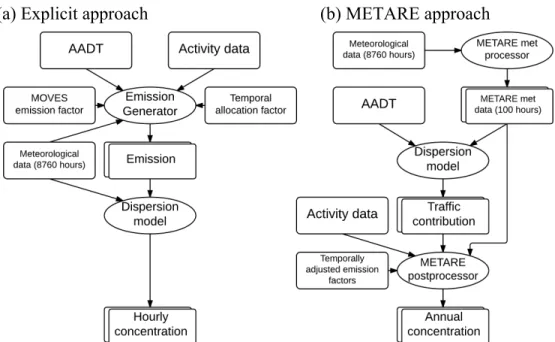
Figure 2.2: Flow charts for (a) the “explicit” approach and (b) the “METARE” 5
approach. The rectangular elements above represent input data, the ovals 6
represent computational programs, and the stacked rectangular elements 7
represent output data. ...18 8
Figure 2.3: Comparison of annual average concentration using the explicit 9
approach versus the METARE approach for (a) unit emissions; (b) CO; (c) 10
NOx; (d) PM2.5 (e) benzene; and (f) formaldehyde. The data points in these 11
figures are from the same receptor group that is mapped to the same NWS 12
site in Cumberland County, ME. The dark bounding lines represent a factor 13
of 2. ...24 14
Figure 2.4: Spatial distribution of the difference (percentage) between the explicit 15
and METARE approaches for the concentrations of (a) CO, (b) NOx, (c) 16
PM2.5, and (d) benzene in Cumberland County, ME. ...26 17
Figure 2.5: Comparison of concentrations for four Detroit measurement sites for 18
the explicit and METARE approaches. (1) Modeled and observed CO for (a) 19
baseline fleet distribution and (c) alternate fleet distribution (composed of 20
fewer HDDV and more LDGV vehicles). (2) Modeled and observed NOx for 21
(b) baseline and (d) sensitivity fleet distribution. The solid lines indicate the 22
1:1 and the factor of 2 intervals. ...28 23
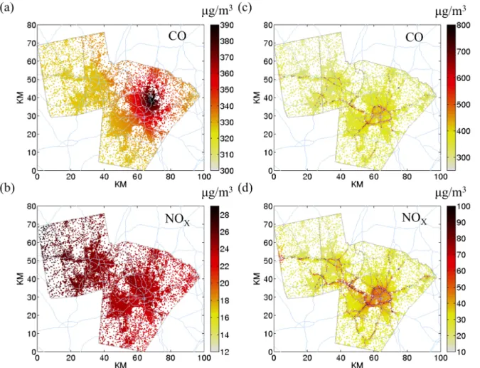
Figure 2.6: Spatial maps of modeled NOx (a and d), PM2.5 (b and e), and Benzene 24
(c and f) concentrations in Cumberland County, ME (left column) and the 25
North Carolina Piedmont region (right column) for 2010. (Note that the color 26
scale differs between CCM and NCP). The color bar represents pollutant 27
concentration in µg/m3. ...32 28
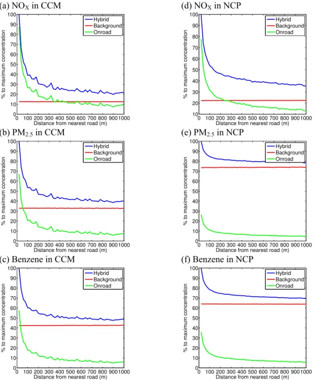
Figure 2.7: Relative contributions of on-road and background concentrations as a 29
function of distance from all roadways, averaged across all receptors for NOx 30
(a and d), PM2.5 (b and e), and Benzene (c and f) in Cumberland County, ME 31
(left column) and the North Carolina Piedmont region (right column) for 32
2010. “Hybrid” is the sum of the background and on-road concentrations. ...36 33
Figure 2.8: Relative contributions of on-road and background concentrations as a 34
function of distance from interstate highways only, averaged across all 35
receptors for NOx (a and d), PM2.5 (b and e), and benzene (c and f) in 36
Cumberland County, ME (left column) and the North Carolina Piedmont 37
region (right column) for 2010. “Hybrid” is the sum of the background and 38
Figure 2.9: The concentration contribution by vehicle type in (a) Cumberland 1
County, ME, and (b) the North Carolina Piedmont. LDGV = light-duty 2
gasoline vehicle, LDGT = light-duty gasoline truck, HDGV = heavy-duty 3
gasoline vehicle, MC = motorcycle, LDDV = light-duty diesel vehicle, 4
LDDT = light-duty diesel truck, and HDDV = heavy-duty diesel vehicle. ...39 5
Figure 2.10: Spatial maps of modeled NOx (a and d), PM2.5 (b and e), and 6
Benzene (c and f) concentration contributions from the HDDV fraction of the 7
fleet distribution in Cumberland County, ME (left column) and the North 8
Carolina Piedmont region (right column) for 2010. (Note that the color scale 9
differs between CCM and NCP). Color bars represent the % contributions. ...43 10
Figure 2.11: Spatial maps of modeled NOx (a and d), PM2.5 (b and e), and 11
Benzene (c and f) concentration contributions from the LDGV fraction of the 12
fleet distribution in Cumberland County, ME (left column) and the North 13
Carolina Piedmont region (right column) for 2010. (Note that the color scale 14
differs between CCM and NCP). Color bars represent the % contributions. ...44 15
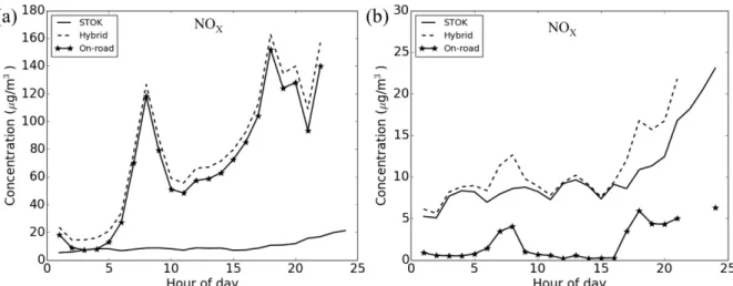
Figure 3.1: Outdoor concentration of CO and NOX at Census block centroids at 16
7:00 AM. (a) CO outdoor STOK (b) NOX outdoor STOK (c) CO outdoor 17
hybrid (d) NOX outdoor hybrid. The color bar represents concentration in 18
µg/m3. (Note that the color scale is different for the four figures to emphasize 19
the concentration ranges that vary by pollutant) ...61 20
Figure 3.2: Hourly pollutant concentration for each Census block in Durham, 21
Orange, and Wake Counties, NC in 2012. (a) CO (b) PM2.5 (c) NOX, and (d) 22
EC. Bottom and top of box represents 25th and 75th percentiles, the line in the 23
middle of the box is the median, the ends of the whisker are the 5th and 95th 24
percentiles, and the dot on the whisker is the mean. ...63 25
Figure 3.3: Spatial CV for each hour (left panel) and Temporal CV for each 26
Census block (right panel). Bottom and top of box represents 25th and 75th 27
percentiles, the line in the middle of the box is the median, the ends of the 28
whisker are the 5th and 95th percentiles, and the dot on the whisker is the 29
mean. ...66 30
Figure 3.4: Time series plot on January 3rd for NOX at (a) a near-road Census 31
block (14.1m from roadway, left panel) and (b) a remote Census block (9.6 32
km from roadway, right panel). ...67 33
Figure 3.5 Indoor concentration of CO and NOX at 7:00 AM with (a) CO indoor 34
STOK (b) NOX indoor STOK (c) CO indoor hybrid (d) NOX indoor hybrid. 35
The color bar represents concentration in µg/m3 (Note that the color scale is 36
different for the four figures to emphasize the concentration ranges that vary 37
Figure 3.6: Indoor-outdoor concentration ratio using mean hybrid concentration at 1
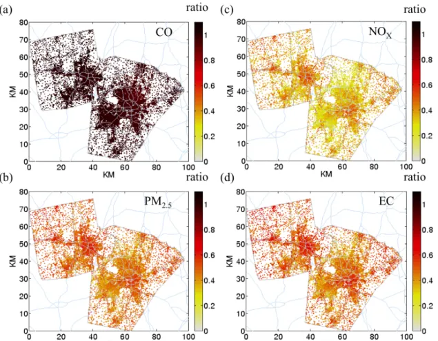
7:00 AM. (a) CO (b) PM2.5 (c) NOX, and (d) EC. ...70 2
Figure 3.7 Hourly normalized difference (ND, left panels) and hourly normalized 3
absolute difference (NAD, right panels) for each Census block. Bottom and 4
top of box represents 25th and 75th percentiles, the line in the middle of the 5
box is the median, the ends of the whisker are the 5th and 95th percentiles, 6
and the dot on the whisker is the mean. ...78 7
Figure 4.1 The NC Piedmont region. The major cities (stars) from left to right: 8
Charlotte, Winston-Salem, Greensboro, and Raleigh. ...87 9
Figure 4.2 Boxplots for modeled annual concentration for total, on-road primary, 10
and on-road secondary PM2.5. Bottom and top of box represents 25th and 11
75th percentiles, the line in the middle of the box is the median, the ends of 12
the whisker are the 5th and 95th percentiles, and the dot on the whisker is the 13
mean. ...96 14
Figure 4.3 Spatial map of annual PM2.5. The colorbar represents concentration 15
level in µg/m3. ...98 16
Figure 4.4 Spatial map of population and premature mortality estiamted using the 17
log-linear CRF. The colorbar represents numer of premature mortality. ...101 18
Figure 4.5 (a) and (b) Normalized on-road primary concentration, its assocaited 19
mortality, and population by distance from the roadways. (c) and (d) 20
Normalized accumulated mortality and population by distance from 21
roadways. The mortality in the figures only is account for on-road primary 22
PM2.5. Mortality (K) represents the estimation using log-linear CRF with RR 23
from Krewski et al. 2009. Mortality (IER) represents the estimation using 24
IER. ...103 25
Figure A1: The modeling domain and the NWS sites used in a) Cumberland 26
County, ME and b) NC Piedmont. The number of each NWS site 27
corresponds to their WBAN numbers. ...115 28
Figure A2: Emission factor variation as a function of temperature in Cumberland 29
County, ME. ...116 30
Figure A3: Emission factor variation as a function of temperature in Mecklenburg 31
County, NC. ...117 32
Figure A4: Emission factor variation as a function of vehicle speed in 33
Cumberland County, ME. ...118 34
Figure A5: Emission factor variation as a function of vehicle speed in 35
Figure A6: Model evaluation in CCM (a and b) and NCP (c) for CO (a and c) and 1
NOX (b). The number at each point is the site ID depicting the Federal 2
Information Process Standard (FIPS) code. The solid lines indicate the 1:1 3
and the factor of 2 intervals. ...120 4
Figure A7: Absolute concentration of on-road source and background as a 5
function of distance from all roadways, averaged across all receptors for NOx 6
(a and d), PM2.5 (b and e), and Benzene (c and f) in Cumberland County, ME 7
(left column) and the North Carolina Piedmont region (right column) for 8
2010. “Hybrid” is the sum of the background and on-road concentrations. ...121 9
Figure A8: Absolute concentration from on-road source and background as a 10
function of distance from interstate highways only, averaged across all 11
receptors for NOx (a and d), PM2.5 (b and e), and benzene (c and f) in 12
Cumberland County, ME (left column) and the North Carolina Piedmont 13
region (right column) for 2010. “Hybrid” is the sum of the background and 14
on-road concentrations. ...122 15
Figure B1. The modeling domain in Durham, Orange, and Wake Counties. ...123 16
Figure B2. Time series plot on January 3rd for CO (a and d), PM2.5 (b and e), and 17
EC (c and f) at a near-road Census block (14.07m from roadway, left panels) 18
and a remote Census block (9.57 km from roadway, right panels). ...124 19
Figure B3. Spatial map for mean AER in (a) spring, (b) summer, (c) fall, and (d) 20
winter. The color bar represents unit in (h-1) ...125 21
Figure C1: Soccer plot comparing modeled and observed PM2.5 with monitoring 22
sites in North Carolina ...129 23
Figure C2: CMAQ model evaluation against monitors in North Carolina (a) 24
normalized mean bias (NMB) and (b) normalized mean error (NME) for 25
PM2.5. ...129 26
Figure C3: Example scatter plots of CMAQ modeled and observed hourly PM2.5 27
concentration n in (a) Wake County and (b) Durham County. The solid line 28
represents 1:2, 1:1, and 2:1 ratio. The subscript obs represents observed 29
value and mod represents modeled value. ...129 30
Figure C4: The scatter plot of CMAQ modeled secondary on-road PM2.5 and the 31
observed secondary on-road PM2.5. The horizontal blue line represents the 32
mean and the vertical blue lines represent the variance of the observation- 33
prediction pair bins. The dashed lines represent the 1 to 2, 1 to 1, and 2 to 1 34
lines. ...132 35
Figure C5: Leave-one-out model evaluation for secondary on-road PM2.5 (a) 36
Figure C6: Example scatter plots of model and observed hourly concentration 1
from the leave-one-out evaluation in (a) Wake County and (b) Durham 2
County. The solid line represents 1:2, 1:1, and 2:1 ratio. The subscript obs 3
represents observed value and mod represents modeled value. ...133 4
Figure C7: Scatter plots of (a) relative risk and (b) Attributable factor for lung 5
cancer to PM2.5 concentration. The log-linear CRF uses epidemiological data 6
from Krewski et al. 2009 ...134 7
CHAPTER 1: INTRODUCTION 1
Transportation plays an important role in the modern society, but it contributes 2
significantly to air pollution. The U.S. Environmental Protection Agency (EPA) estimated that 3
on-road emission contributes 54.8%, 5.5%, and 39% to anthropogenic emissions of nitrogen 4
oxides (NOx), particulate matter with diameter smaller than 2.5 𝜇𝑚 (PM2.5), and benzene 5
respectively (Fig. 1.1). Further, a previous study has shown that on average, 19% of the U.S. 6
population lives close to high-traffic roadways and in some counties, this percentage can be up to 7
79% (Rowangould, 2013). This implies that a large portion of the U.S. population lives in the 8
proximity of a major source of air pollution (i.e. roadways) and has the potential to be exposed to 9
high level of air pollutants. 10
Fig. 1.1: Emission contribution for NOx, PM2.5, and Benzene in the U.S. Source: U.S. EPA emission inventory
45.2
94.5
61.0 54.8
5.5
39.0
NOx
PM2.5
BENZENE
on-road emission % in U.S. 2012
Traffic-related air pollutants can cause adverse effects on public health (Gauderman et al. 1
2007; Baccarelli et al. 2009; Lindgren et al. 2010; McConnell et al. 2010; Künzli 2014; Urman et 2
al. 2013). For example, several studies have shown that near-road exposure to traffic related air 3
pollutants is associated with increasing prevalence of asthma in adults (Lindgren et al., 2010) and 4
increasing incidence of asthma in children (McConnell et al., 2010). A recent study has further 5
pointed out that exposure to traffic-related air pollutants including nitrogen dioxide (NO2), NOx, 6
and carbon monoxide (CO) is associated with tuberculosis (Lai et al., 2015). These studies, 7
however, focused on a relatively smaller cohort. To address the concern on public health at a 8
population level and to quantify the impact (such as premature mortality or economical loss) on 9
human society, it is essential to characterize near-road exposure to traffic-related air pollutants at 10
regional to national scales. 11
Estimating exposure to traffic-related air pollutants is challenging because of dynamic 12
traffic conditions, multiple pollutants, the need to separate near-road and regional pollution, and 13
the spatial and temporal resolution needed to document pollutants. Traditionally, field 14
measurements, statistical modeling, and emissions-based air quality modeling have been used to 15
overcome the challenges and quantify the impact of transportation on air quality. Land use 16
regression models (LUR), for example, combines field measurements and statistical methods to 17
capture the spatio-temporal variation of traffic related air pollutants. Lindström et al. (2013) used 18
this type of technique to combine field measurements in Los Angeles, California and a line- 19
source dispersion air quality model to estimate the ambient concentration level of traffic-related 20
air pollutants. Conducting a field sampling campaign to cover a large domain to support LUR 21
modeling, however, requires a large amount of time and costly sampling devices. Although field 22
their spatial resolution and coverage is limited due to the amount of available monitors or the 1
cost associated with them. 2
Another approach to quantify exposure to traffic-related air pollutants is with emission- 3
based air quality models. This type of model predicts air quality based on current knowledge of 4
physics and chemistry about the atmosphere and can cover a large area with arbitrary spatial 5
resolution. These models can be categorized as chemical transport models (CTM) (Byun and 6
Schere, 2006a), dispersion models (Cimorelli et al., 2005; Snyder et al., 2013), and hybrid 7
models (Isakov et al., 2009; Stein et al., 2007). Compared with measurement-based approaches, 8
emissions-based modeling has a greater capability to connect emissions from on-road activity to 9
resultant pollutant level because of its ability to distinguish between source types during the 10
modeling process. This is critical for implementing mitigation strategies. In the U.S., Fann et al. 11
(2013), and Caiazzo et al (2013) used detailed CTMs and estimated that mobile sources are 12
either the second largest sector to cause ozone- and PM2.5-related premature deaths (~29,000 per 13
year) or the largest sector causing premature deaths due to PM2.5 (53,000 per year) and ozone 14
(5,000 per year). Both these studies highlight the growing importance of health risk due to 15
mobile source emissions. 16
Although previous studies were able to predict some compelling risk estimates at a 17
population level, the application of CTM might have biased the resultant premature mortality 18
estimate due to its limited spatial resolution. A previous monitoring-based study has shown that 19
traffic-related air pollutants could reduce by more than 50% within 150 meters from roadways 20
(Karner et al., 2010). Also, another study has shown that children living close to major highways 21
(<500 m) show a significant decrease in forced expiratory volume in the first second (FEV1) 22
Because 19% of the U.S. population lives close to heavy-traffic roadways (Rowangould, 2013), 1
it is important to identify the pollutant hotspot near roadways. With CTMs, the modeling domain 2
is divided into several “grids” and the air pollutant concentration within each grid is assumed to 3
be distributed homogenously. The CTM then solves the differential equation derived from mass 4
balance theory to obtain the concentration for each grid. As such, the number of the grid 5
determines the spatial resolution of a CTM. At a national scale application, CTM is usually 6
implemented at a 36-km × 36-km or 12-km × 12-km resolution. Therefore, the concentration 7
hotspot within 150 meters from the roadways cannot be captured, and the near-road impacts are 8
substantially diluted within the larger grid volume. Although CTMs can be implemented at a 9
high spatial resolution (i.e. smaller grid sizes), it would significantly increase the computational 10
burden due to the increased number of grid cells. Using CTMs at relatively coarse spatial 11
resolutions (36-km × 36-km and 12-km × 12-km) however, can limit the ability to determine the 12
locations of specific high-risk areas in population risk assessments (Arunachalam et al., 2011, 13
2006). 14
An alternative for fine-resolution modeling is using dispersion models. When compared 15
to a CTM, a Gaussian plume dispersion model is relatively simple and computationally efficient. 16
Compared to CTMs, dispersion models do not require allocating emissions from roadways to 17
grids that are consistent with CTMs’ modeling grids. In a dispersion model, the emission source 18
is allocated in a much finer spatial resolution more realistically retaining the shape and physical 19
characteristics of the emitted plume. For example, dispersion models can model roadways as 20
adjacent area sources (Cook et al., 2008; Crooks and Isakov, 2013; Stein et al., 2007) or line 21
sources (Batterman et al., 2014a; Chang et al., 2015a; Heist et al., 2013). Thus, the sharp 22
al., 2015b; Isakov et al., 2014). Modeling TRAPs with dispersion models can still be challenging 1
due to the demand to characterize a temporally refined emission for each roadway. This link- 2
based emission can be obtained with a “bottom-up” approach (Cook et al., 2008; Isakov et al., 3
2009; Snyder et al., 2014), but require detailed information including: geometry of the road 4
network, traffic activity, temporal allocation factor (Batterman et al., 2015), emission factors of 5
pollutants, and meteorology. This kind of technique, to our knowledge, has only been applied in 6
smaller geographical areas such as at city (Beevers et al., 2013; Lobdell et al., 2011) or 7
community (Wu et al., 2009) level or with subject-specific health studies (Vette et al., 2013). 8
Only a few studies have applied the bottom-up approach for a large spatial domain to create 9
exposure estimates for a burden of disease assessment. These results, however, were not 10
compared with the traditional CTM approach (Ghosh et al., 2015). Further, unlike a CTM, a 11
Gaussian dispersion model is unable to predict secondary pollutants such as ozone or secondary 12
PM2.5 formed from atmospheric chemical reactions. Because the majority of ambient PM2.5 in the 13
atmosphere is secondary (Jimenez et al., 2009; Kleindienst et al., 2010; Seinfeld and Pandis, 14
2006; Zhang et al., 2007), using a Gaussian plume dispersion model may underestimate the total 15
impact of on-road PM2.5. 16
Besides the required spatial resolution, another important factor to accurately estimate 17
exposure to air pollutant is the indoor concentration from outdoor origins. In many heath studies, 18
exposure to air pollutants are often estimated based on ambient concentration level (Anderson et 19
al., 2013a, 2013b; Lindgren et al., 2010; McConnell et al., 2010). Ambient concentration 20
collected from fixed-site monitors, for example, provides regional concentration and can be used 21
to determine inter-city difference (Dockery et al., 1993). Fixed-site monitors, however, are often 22
across space. For pollutants with local sources such as on-road vehicular emission, the data from 1
fixed-site monitors can fail to capture the intra-urban variation(Jerrett et al., 2005) resulting in 2
exposure misclassification (K. L. Dionisio et al., 2013). 3
A more accurate method for estimating personal exposure is with direct measurements 4
using personal sampling devices (Michikawa et al., 2014; Van Roosbroeck et al., 2006). For 5
example, Delfino et al.(2004) compared the association between the reduction in forced 6
expiratory volume in the first second (FEV1) of asthmatic children and four particulate matter 7
(PM) exposure metrics: personal sampling device, indoor concentration at home, outdoor 8
concentration at home, and data from central monitor. The results showed that the reduction in 9
FEV1 is more strongly associated with personal PM exposure or concentration collected indoor 10
at home than concentration collected at a central monitoring site or outdoor concentration at 11
home. Although personal sampling devices can best represent total exposure, they are costly and 12
introduce participant burden for individuals in health studies. 13
One approach that could be used for exposure assessment using a large spatial domain is 14
with model-based exposure metrics. They are less costly and can cover a wider spatial domain. 15
These exposure metrics can be obtained from various approaches such as space-time kriging, air 16
quality modeling, and land use regression. These approaches, when compared to fixed-site 17
monitors, can increase the potential in predicting intra-urban spatial variability. Space-time 18
kriging technique interpolates observational data to provide spatiotemporally refined 19
concentrations (Arunachalam et al., 2014; de Nazelle et al., 2010). These estimated ambient 20
concentrations can then be used to relate to adverse health effects (Coogan et al., 2012; Lee et 21
al., 2013, 2011). Nevertheless, studies have found that indoor concentrations would be a better 22
Roosbroeck et al., 2006). The Windsor, Ontario Exposure Assessment study has shown that 1
children spend on average more than 67% of their time indoors and receive more than 50% of 2
their PM2.5 exposure while indoors (Van Ryswyk et al., 2014). Also, previous studies have 3
pointed out that the variation of air exchange rate (the rate that indoor air is exchanged with 4
outdoor air) can further explain the difference in ozone mortality coefficient across cities (Chen 5
et al., 2012) and acute air pollution-related morbidity (Sarnat et al., 2013) than using outdoor air 6
pollutant concentration from central monitoring sites alone. The approaches for modeling indoor 7
concentration have been developed and evaluated (Hering et al., 2007; Hodas et al., 2014; Zauli 8
Sajani et al., 2015) primarily for subject-specific health study(Vette et al., 2013). To our 9
knowledge, these approaches have not been used to provide spatial and temporally refined 10
estimates for predicting personal exposure because house-by-house information required for 11
predicting AER is difficult to obtain in a large domain without house-by-house survey. 12
In this work, we explored the possibility to apply air quality models to estimate traffic- 13
related air pollutant levels for risk and exposure studies. To better characterize the near-road 14
exposure, we developed a modeling framework to allow fine-resolution modeling for traffic- 15
related air pollutants. To quantify the potential exposure error, we developed and evaluated 16
multiple exposure metrics built with air quality models. To estimate the potential bias due to the 17
limitation in CTM approaches to estimate on-road PM2.5 related mortality, we compared the 18
mortality estimate from CTM at a courser spatial resolution and a newly developed hybrid 19
modeling method at a fine resolution. 20
1
CHAPTER 2: A MODELING FRAMEWORK FOR CHARACTERIZING NEAR-ROAD 2
AIR POLLUTANT CONCENTRATION AT COMMUNITY SCALES1 3
2.1 Introduction 4
Transportation plays an important role in modern society, but its impact on air quality can 5
have significant adverse effects on public health, as numerous studies have shown (Gauderman 6
et al. 2007; Baccarelli et al. 2009; Lindgren et al. 2010; McConnell et al. 2010; Künzli 2014; 7
Urman et al. 2013). Because 19% of the U.S. population lives near heavy-traffic roads, and this 8
group includes larger shares of both nonwhite residents and lower median household incomes 9
(Rowangould, 2013), it is essential to characterize near-road exposure to address concerns about 10
public health and environmental justice. 11
Accurate characterization of exposure to air pollution from traffic is also important for 12
environmental epidemiologic studies (Lobdell et al., 2011; Vette et al., 2013). However, 13
estimating near-road exposure is challenging because of dynamic traffic conditions, multiple 14
pollutants, the need to separate near-road and regional pollution, and the spatial and temporal 15
resolution needed to document pollutants. Traditionally, field measurements, statistical 16
modeling, and emissions-based air quality modeling have been used to overcome the challenges 17
and quantify the impact of transportation on air quality. Land-use regression (LUR) models have 18
also been used to capture spatial variation of traffic-related pollutants. An example can be seen in 19
Lindström et al. (2013) where data collected from multiple monitors and a line source dispersion 20
1This chapter previously appeared as an article in Science of the Total Environment. The original
citation is as follows: Chang, S.Y., Vizuete, W., Valencia, A., Naess, B., Isakov, V., Palma, T.,
model are combined using a spatio-temporal framework to estimate ambient concentrations. 1
However, conducting a sampling campaign for a large domain in support of LUR modeling 2
would require a significant number of samplers, which would be costly and time consuming. 3
Therefore, although field measurements and statistical models can provide concentration 4
information with greater certainty and identify the main contributors to pollutant levels, the 5
spatial resolution and coverage may be insufficient due to the limited number of available 6
monitoring devices or the costs associated with them. 7
Another approach to characterize traffic-related air pollutants is using emissions-based air 8
quality models. These models can predict pollutant concentrations over a larger domain with 9
arbitrary spatial resolution by combining emissions data and current knowledge about physical 10
and chemical processes in the atmosphere. These models can be categorized as chemical- 11
transport models (Caiazzo et al., 2013), dispersion models (Lobscheid et al. 2012; Venkatram et 12
al. 2007), and hybrid models (Isakov et al. 2009; Stein et al. 2007). Compared with 13
measurement-based approaches, emissions-based modeling has a greater capability to connect 14
emissions from on-road activity to resultant pollutant level because of its ability to distinguish 15
between source types during the modeling process. This is critical for implementing mitigation 16
strategies. In the U.S., Fann et al. (2013), and Caiazzo et al (2013) used detailed chemistry 17
transport models and estimated that mobile sources are either the second largest sector to cause 18
ozone- and PM2.5-related premature deaths (~29,000 per year) or the largest sector causing 19
premature deaths due to PM2.5 (53,000 per year) and ozone (5,000 per year). Both these studies 20
highlight the growing importance of health risk due to mobile source emissions. Nevertheless, 21
while these analyses were able to predict some compelling risk estimates, the relatively coarse 22
ability to determine the locations of specific high-risk areas in population risk assessments 1
(Arunachalam et al., 2011, 2006). To identify and quantify high-risk areas requires high- 2
resolution and large-scale modeling, which is computationally intensive. In addition, quantifying 3
the contribution from a single source would generally require running the model multiple times, 4
which further increases the computational burden. 5
In our study, we developed a hybrid modeling approach that includes the Research LINE 6
source dispersion model (R-LINE) (Snyder et al., 2013) for modeling traffic-related 7
concentrations and ambient observed data as a source for regional background concentrations at 8
fine resolution (i.e., at Census-block level) in a computationally efficient manner (i.e., within 9
minutes). We modified the "bottom-up" strategy (Cook et al., 2008)—under which the emissions 10
are accurately represented by each roadway's actual location—to estimate near-road exposures 11
on a large scale while resolving near-road gradients. The approach has been evaluated with an 12
explicit simulation (the bottom-up method) for Portland (Cumberland County), ME, and the 13
model performance has been evaluated against a near-road monitoring study in Detroit, MI, 14
conducted by the EPA and the Federal Highway Administration (FHWA) (Vallero et al., 2013). 15
The novelty of our approach, when compared to prior methods, is the combination of 16
traffic-related contributions using R-LINE with a spatio-temporal kriging method to obtain 17
background concentrations before implementing an approach to run only select hours of the year 18
to compute annual averages (thus providing critical savings in computational time), while 19
incorporating temporal variability of traffic-related emissions. We give two illustrative examples 20
that involve applying the modeling framework in two geographical areas: Cumberland County, 21
ME, and North Carolina's Piedmont region. Cumberland County (denoted as CCM) (Fig 2.1a) 22
as NCP) (Fig 2.1b), as representative for a larger domain with both metropolitan and rural areas 1
included. These two were also chosen to demonstrate contrast between two regions of the 2
(a)
(b)
Figure 2.1: The modeling domains in a) Cumberland County, Maine (CCM) and b) North Carolina Piedmont (NCP).
1
2.2 Methods 1
2.2.1 Modeling framework 2
The modeling framework is composed of two major components: On-road concentration 3
(Sections 2.2.2 and 2.2.3) and urban background concentration (Section 2.2.4). In this approach 4
we assume that modeled concentrations at selected locations (i.e., Census-block centroids) can 5
be used to estimate population exposure in support of exposure and health studies. Therefore, the 6
concentrations from the two components are estimated at Census-block centroids and the 7
summation of the two components is the total ambient concentration. Although concentration 8
fields at parcel level may likely serve as a better exposure metric, previous studies have shown 9
that the difference in mean and maximum concentrations between parcel and Census block level 10
only ranges from -2.4 to 7.1% (Batterman et al., 2014b; Wu et al., 2009). The EPA is currently 11
utilizing Census-block centroids as health risk estimation points in its residual risk program (U.S. 12
Environmental Protection Agency, 2009), which allows continuity between studies. 13
We employed R-LINE (Snyder et al., 2013) to estimate near-road concentrations, because 14
this model treats roads as line sources and applies new formulations for horizontal and vertical 15
plume spread (Venkatram et al., 2013). The transportation data required to estimate emission 16
includes road networks (individual road segment locations), traffic activity (number of vehicles 17
for each road segment over a period of time), and traffic speed. Meteorological datasets include 18
hourly observations for the study period from multiple National Weather Service (NWS) stations 19
covering the study domain. These sites were chosen based on their distances to the Census-block 20
centroids within the domain; each centroid was mapped to the nearby NWS sites, and the site 21
that yielded the shortest distance was chosen to provide meteorological information. Table 2.1 22
We used AERMINUTE to process 1-minute wind speed data from the Automated Surface 1
Observations Stations (ASOS) network (http://www.nws.noaa.gov/ost/asostech.html), followed 2
by AERMOD's meteorological processor AERMET (version 13350) to provide necessary 3
meteorological inputs for the dispersion calculations used to estimate near-road exposures in 4
Detroit, MI; CCM; and NCP. At the time the meteorological inputs were prepared, AERMET did 5
not have a feature to adjust for surface friction velocity (u*); therefore, we used a post processor 6
that applies the algorithm described in Qian and Venkatram (2011) to adjust for u*. 7
NCP and CCM were modeled with meteorological data from 14 and 3 NWS sites, 8
respectively. The NWS sites provide hourly meteorological information from 2009 to 2011 for 9
NCP and from 2011 for CCM. The model receptors in CCM and NCP were set at Census-block 10
centroids, resulting in 6,509 receptors in CCM and 104,759 receptors in NCP. The average size 11
of the Census block is 0.38±1.64 km2 in CCM and 0.33±0.99 km2 in NCP. In Detroit, we 12
evaluated R-LINE at four near-road monitoring sites for a study period from September 2010 to 13
June 2011, a range that was time-matched with the sampling period used to evaluate the model 14
performance. This study was designed to evaluate the computational resources and the feasibility 15
for expanding our efforts to a nationwide application to develop high-resolution fields of 16
concentration due to near-road traffic activity. 17
We developed and applied our method for the following list of pollutants: 18
• Carbon monoxide (CO), nitrogen oxides (NOx) and fine particulate matter (PM2.5) 19
• Five mobile-source air toxics (MSATs): acetaldehyde, acrolein, benzene, 1,3-butadiene, 20
and formaldehyde 21
Table 2.1: National Weather Service sites included in this study. 1
Domain WBANa Number Surface Site Name
NC Piedmont
03810 Hickory FAA Airport
13722 Raleigh Durham WSFO Airport 13723 Greensboro WSO Airport 13728 Danville Regional Airport 13881 Charlotte WSO Airport 53870 Gastonia Municipal Airport
53871 Rock Hill York County Bryant Field Airport 53872 Monroe Airport
93740 Fayette Regional/Grannis Field Airport 93759 Rocky Mount-Wilson Regional Airport 93782 Laurinburg-Maxton Airport
93783 Burlington Alamance Regional Airport 93785 Horace Williams Airport
93807 Smith Reynolds Airport Cumberland
County, ME
14764 Portland City Airport 54772 Fryeburg E Slopes Airport 94623 Wiscasset Airport
Detroit, MI 14822 Detroit City Airport
aWeather-Bureau-Army-Navy 2
3
4
2.2.2 Emissions and the explicit modeling approach 5
We used the Motor Vehicle Emission Simulator 2010b (MOVES2010b)(U.S. 6
Environmental Protection Agency, 2012) to retrieve county-based roadway emission factors with 7
units of grams per mile per vehicle. The emission factors are grouped based on the following: 8
• There are 12 road type categories: rural interstate, rural principal arterial, rural minor 9
arterial, rural major collector, rural minor collector, rural local, urban interstate, urban 10
freeway, urban principal arterial, urban minor arterial, urban collector, and urban local. 11
• Vehicle speed is categorized using 16 bins (in mi/h): <2.5, 2.5 to 5, 5 to 10, 10 to 15, 15 12
to 20, 20 to 25, 25 to 30, 30 to 35, 35 to 40, 40 to 45, 45 to 50, 50 to 55, 55 to 60, 60 to 13
• The ambient temperature is binned based on the actual ambient temperature of the 1
counties simulated, using an interval of 5°F. 2
• MOVES groups vehicles based on fuel type and gross vehicle weight rating (GVWR). 3
This results in 12 vehicle types: light-duty gasoline vehicle (LDGV), light-duty 4
gasoline truck with GVWR between 0 and 3750 lbs. (LDGT1), light-duty gasoline 5
truck with GVWR between 3751 and 5750 lbs. (LDGT2), heavy-duty gasoline truck 6
(HDGT), light-duty diesel vehicle (LDDV), light-duty diesel truck (LDDT), heavy-duty 7
diesel vehicle (HDDV), and motorcycle (MC). Heavy-duty diesel vehicle is further 8
categorized by GVWR, which includes Class 2B; Class 3, 4, and 5; Class 6 and 7; Class 9
8A and 8B; and school bus. 10
The percent change in emission factor variation as a function of temperature, vehicle speed, and 11
vehicle type can be found in Figs. A2 to A5. 12
Estimating nationwide traffic-related air pollutant level requires emission factors for all 13
counties in the U.S. To reduce the computational burden for MOVES when generating these 14
emission factors, reference counties were used. 146 reference counties were selected to represent 15
a set of counties that are similar in their characteristics (e.g., urban or rural) and meteorology 16
(e.g., temperature) (Zubrow, 2012). Similarly, reference fuel months were used to represent a set 17
of months with similar emission patterns; January represents February to April and October to 18
December, and July represents May to September. 19
Since MOVES provides countywide emission factors as a function of road type, vehicle 20
speed, ambient temperature, and vehicle type, the emission rate from a specific roadway is 21
calculated as follows: 22
𝐸!",! = !" 𝑇𝐶!,!×𝐸𝐹(𝑉𝑇!,𝑇!,𝑆𝑃!,𝑅𝑇)
where E is the emission rate of the line source, TC is the traffic count, EF is the emission factor, 1
VT is the vehicle type, T is the ambient temperature, SP is the vehicle speed, RT is the road type 2
from 1 to 12, h is the hour index, and i is the vehicle type index from 1 to 12. 3
The information required for calculating the emission rate was gathered from multiple 4
sources. The roadway information—including road coordinates, road type, and annual average 5
daily traffic (AADT)—was taken from the FHWA Freight Analysis Framework Version 3 6
(FAF3) (Federal Highway Administration, 2012a). The roadway information provided in FAF3 7
contains curved and long road segments. R-LINE assumes each road to be a straight line, so we 8
split the original roadways into several segments with start and end points at the vertices of the 9
roadway. We assigned MOVES-based emissions factors to all road links provided by FAF3, but 10
we do note that some local roads were missing in FAF3, and hence were unmodeled. FAF3 11
provides AADT data that are aggregated across all vehicles. To disaggregate these data based on 12
vehicle types, we first used Table VM-4 from FHWA's Highway Statistics (Federal Highway 13
Administration, 2012b), which summarizes the distribution of annual vehicle distance traveled, 14
to obtain the fraction of the AADT data in each of six Highway Performance Monitoring System 15
(HPMS) vehicle classes. The HPMS classes were then converted to MOVES vehicle types based 16
on the EPA's Emission Inventory Improvement Program (Decker et al., 1996). Because the fleet 17
break down calculation does not further categorize HDDV, we compare the emission factor table 18
against the emission factor used in a previous study, where HDDV is not further categorized 19
(Snyder et al., 2014) and use HDDV school bus to represent HDDV emission for NOx and 20
HDDV Class 8A and 8B to represent HDDV for other pollutants. The AADT data were then 21
distributed based on the eight fractions (Tables A1 and A2) to obtain the AADT for each vehicle 22
temporal allocation factors. The temporal allocation factors were obtained from EPA’s National 1
Emission Inventory and Sparse Matrix Operator Kernel Emissions (SMOKE) (Houyoux et al., 2
2000), which summarizes the distribution of traffic by month of a year, day of a week, and hour 3
of a day by weekday and weekend. The temperature was obtained from the closest NWS site 4
(chosen as described in Section 2.1.1). The vehicle speed was taken from the MOVES input file, 5
which contains county-based vehicle speed grouped by road type and vehicle type. 6
The explicit modeling (Fig. 2.2a) adopted the bottom-up approach (Cook et al., 2008). 7
Under this approach, we developed an Emission Generator utility in Fortran that processes data 8
that include traffic counts, road-link-specific activity data (including vehicle speed and road 9
type), MOVES emission factors, and meteorological data to calculate the hourly emission rate of 10
each road link based on Eq. 1. The generated emission rates were then combined with 11
meteorological data and used as input for R-LINE to compute hourly pollutant concentrations. 12
(Fig. 2.2b is discussed in the next section.) 13
(a) Explicit approach (b) METARE approach
Figure 2.2: Flow charts for (a) the “explicit” approach and (b) the “METARE” approach. The rectangular elements above represent input data, the ovals represent computational programs, and the stacked rectangular elements represent output data.
2.2.3 The METeorologically-weighted Averaging for Risk and Exposure (METARE) approach 1
Using the explicit approach to model multiple pollutants at Census-block level at hourly 2
resolution is very computationally intensive because the dispersion model needs to be run 3
multiple times for each pollutant and for each hour modeled. To provide a less burdensome 4
method, we developed another bottom-up method, the METARE approach (Fig. 2.2b). 5
Because all of the traffic-related pollutants come from the same source, we used the AADT 6
(instead of the emission rate) as the emission input to be dispersed to all receptors. The output, 7
traffic contribution dispersed from roadways, was then used in conjunction with target pollutants' 8
emission factors to obtain hourly concentration using the following equation: 9
𝐶!,! = ! !𝑇!𝐶!,!,!×𝑎𝑑𝑗𝐸𝐹!(𝑉𝑇!,𝑇!,𝑆𝑃!,𝑅𝑇!)
!!! (2.2) 10
where C is the concentration at a receptor, TrC is the traffic contribution from roadways, adjEF 11
is the adjusted emission factor by temporal allocation factors, VT is the vehicle type, T is the 12
ambient temperature, SP is the vehicle speed, RT is the road type from 1 to 12, h is the hour 13
index, i is the vehicle type index from 1 to 8, s is the source index, and p is the pollutant index. 14
Compared to U.S. EPA’s STAR approach, METARE uses the adjusted emission factor to adjust 15
for the temporal variability and calculates a representative emission factor for each METARE 16
meteorological group. By doing so, the temporal variation in traffic emissions can be captured 17
adequately with METARE, while STAR is more suitable for emission sources that have less 18
diurnal variability. 19
With Eq. 2, the dispersion model needs to be implemented only once to provide the traffic 20
contribution from each source (TrCi,h,s). However, saving all of this information would require 21
enormous computational resources. We therefore simplified the process by grouping the 22
type to provide road-type-specific traffic contributions at each receptor. The total concentration 1
was then calculated as: 2
𝐶!,! = !" 𝑇𝑟𝐶!,!,!"×𝑎𝑑𝑗𝐸𝐹!(𝑉𝑇!,𝑇!,𝑆𝑃!,𝑅𝑇)
!"!! !
!!! (2.3) 3
where TrCi,h,RT represents the hourly traffic contribution for vehicle type i on road type RT. With 4
this method, R-LINE is run for up to 12 times, once for each roadway type, and the METARE 5
postprocessor (see Fig. 2.2b) is used to calculate the concentrations for multiple pollutants based 6
on corresponding emission factors. 7
Annual average concentration is often used to represent long-term exposure (Gauderman et 8
al., 2007). Using the explicit approach to obtain annual concentrations for one year would 9
require 8760 hours (365 days×24 hours/day) of meteorological input. To further reduce the 10
computational burden in the METARE approach, we adopted a method that is similar to EPA's 11
STability ARray program (STAR) method (U.S. Environmental Protection Agency, 1997) to 12
estimate annual average concentrations using a set of representative meteorological conditions. 13
These conditions represent a set of meteorological inputs with similar wind speed, wind 14
direction, and Monin-Obukhov length. Each of these three parameters was divided into several 15
bins (Table 2.2), and the hour with median Monin-Obukhov length in each bin was chosen as the 16
representative hour. The combination of the meteorological parameter bins yields 100 groups, 17
each represented by one hour of meteorological conditions. The METARE met processor 18
implements this process (see Fig. 2.2b). The adjusted emission factor (adjEF in Eq. 4) in this 19
case is the average of the adjusted emission factors in each group. The weight (i.e., the number 20
of hourly meteorological data in a group divided by the total number of hours of meteorological 21
conditions) was used to scale the concentration output from the 100 hours of meteorological 22
𝐶! = !""𝐶!×𝑊!
!!! (2.4) 1
where CA is the annual concentration, Cr is the concentration output from the representative 2
meteorological condition, Wr is the weight, and r is the group index. 3
Table 2.2: The meteorological bin used in METARE approach 4
Parameter Bin
Wind speed (m/s)
0 to 1 1 to 2 2 to 4 4 to 7 > 7
Wind direction (degree)
0 to 90 90 to 180 180 to 270 270 to 360
Monin-Obukhov length
0 to 100 (stable)
100 to 500 (slightly stable) > 500 or <-500 (Neutral) -500 to -100 (slightly unstable) -100 to 0 (unstable)
5
2.2.4 Background Concentrations 6
The R-LINE model is designed to calculate near-road concentrations from traffic emissions and 7
therefore can capture the on-road mobile-source contribution to local air quality but not the 8
regional background and the contributions from other sources (referred to as “urban 9
background”). The background contribution can be very significant, depending on the pollutant 10
and the geographical area (K. Dionisio et al., 2013). However, accurately characterizing the 11
urban background contribution for estimating total exposure can be resource intensive (Crooks 12
and Isakov, 2013). Observations from AQS sites have been used to provide background in 13
NATA, wherein, the quality of the collected ambient monitoring data is used to determine 14
Agency, 2011). In our approach, we estimated the urban background concentration using the 1
Space-Time Ordinary Kriging (STOK) technique (Zimmerman and Zimmerman, 1991). STOK 2
uses available monitoring data from two monitoring networks (Air Quality System and Chemical 3
Speciation Network (U.S. Environmental Protection Agency, 2013)) to interpolate observational 4
data at Census-block centroids. This technique assumes that the concentration value at each 5
estimation point is a linear combination of nearby "hard data" (i.e., the observational data). The 6
linear combination, also known as kriging weight, is determined by minimizing the estimation 7
variance while satisfying the unbiased constraint. The STOK technique is implemented with 8
BMElib (Bayesian Maximization Entropy library) (Serre, 1999). A detailed description of the 9
STOK algorithm, which was developed and applied for the Near-road Exposures to Urban Air 10
Pollutants Study (NEXUS) (Vette et al., 2013) in Detroit, MI, can be found in Arunachalam et al. 11
(2014). We applied this algorithm from Arunachalam et al. (2014) to estimate hourly background 12
concentrations at all receptors in each of the study domains. 13
14
2.3 Results and Discussion 15
2.3.1 Method and model evaluation 16
Because the great temporal variation in emission for traffic related air pollutants could 17
affect METARE’s performance, we first used an inert pollutant with unit emission rate (i.e., 1 18
g/mi/s) as input to R-LINE to evaluate the METARE method’s performance. Fig. 2.3a compares 19
the METARE and explicit approaches for Cumberland County, ME when using unit emission 20
rate. The two runs agree well, with slight underestimation when the concentration is high. The 21
normalized mean bias (NMB) is -9.53% and the normalized mean error (NME) (Boylan and 22
Figs. 2.3b through 3f show five examples (CO, NOx, PM2.5, benzene, and formaldehyde) of 1
the comparison between the METARE and explicit approaches for the same domain when using 2
actual pollutant-specific emissions. For the five pollutants, the difference is always within a 3
factor of 2, with slight underestimation. Table 2.3 shows the NMB and NME between the two 4
approaches, using results from the explicit method as the standard. For all of the pollutants, NME 5
ranges from 12.58 to 14.54% and NMB ranges from -11.25 to -12.98%, indicating a good match 6
between the two methods. Compared with the test case where unit emission is used as input, the 7
performance was worse because of the temporal variation of the emissions. Nevertheless, the 8
additional error and bias ranged from 2 to 5%, which is relatively modest. It is worth noting that 9
the coefficients of determination for all pollutants exceed 0.98, indicating a high correlation 10
(a) (b)
(c) (d)
(e) (f)
Figure 2.3: Comparison of annual average concentration using the explicit approach versus the METARE approach for (a) unit emissions; (b) CO; (c) NOx; (d) PM2.5 (e) benzene; and (f) formaldehyde. The data points in these figures are from the same receptor group that is mapped to the same NWS site in Cumberland County, ME. The dark bounding lines represent a factor of 2.
1
2
0 0.05 0.1 0.15 0.2
0 0.05 0.1 0.15 0.2 Unit emission Explicit run ASWIC MET AR E Unit emission
0 100 200 300 400 500 600
0 100 200 300 400 500 600
Explicit run (µg/m3)
METARE (
µ
g/m
3 )
CO
0 50 100 150 200
0 50 100 150 200
Explicit run (µg/m3)
METARE (
µ
g/m
3 )
NOx
0 2 4 6 8 10
0 2 4 6 8 10
Explicit run (µg/m3)
METARE ( µ g/m 3 ) PM 2.5
0 0.2 0.4 0.6 0.8
0 0.2 0.4 0.6 0.8
Explicit run (µg/m3)
METARE (
µ
g/m
3 )
Benzene
0 0.2 0.4 0.6 0.8
0 0.2 0.4 0.6 0.8
Explicit run (µg/m3)
METARE (
µ
g/m
3)
Table 2.3: Performance metrics for METARE using the explicit approach as the standard 1
Species NMBa (%) NMEb (%) R2 c
Unit emission -9.53 10.46 0.99
Formaldehyde -11.58 13.12 0.99
1,3-Butadiene -11.25 12.72 0.98
Acetaldehyde -11.69 13.16 0.99
Benzene -11.23 12.71 0.98
Acrolein -11.47 13.10 0.99
NOx -11.52 12.84 0.99
CO -11.29 12.58 0.99
PM2.5 -12.98 14.54 0.98
aNormalized mean bias: !!!!(!!!!!) !! !
!!! . Co: explicit modeled concentration, Cm: modeled 2
concentration. 3
bNormalized mean error: !!!!|!!!!!| !! !
!!! . Co: explicit modeled concentration, Cm: modeled 4
concentration. 5
cCoefficient of determination: 1− !!!!! !!!!! !
!!!!! !!!!! !. Cm: modeled concentration, fm: value from 6
regression line. 7
Fig. 2.4 shows the spatial distributions of the concentration differences as percentages for the 1
Cumberland County, ME, domain. The four example pollutants show similar patterns where, 2
overall, the difference is moderate except for the overprediction in the northeast part of the 3
domain (in red) and underprediction in the southeast part of the domain (in blue). These less 4
accurate regions have lower concentrations. In these regions, a small variation in wind direction 5
or emission can easily cause huge difference although the absolute concentrations are still low. 6
(a) CO (b) NOx
(c) PM2.5 (d) Benzene
Figure 2.4: Spatial distribution of the difference (percentage) between the explicit and METARE approaches for the concentrations of (a) CO, (b) NOx, (c) PM2.5, and (d) benzene in Cumberland County, ME.
7
We evaluated the model’s ability to estimate near-road pollution gradients using data from a 8
recently conducted field study in Detroit, MI (Vallero et al., 2013). Air quality measurements 9
were conducted at four monitoring sites near Interstate 96 (I-96) in Detroit. These monitoring 10
0 20 40 60 80
0 20 40 60 KM KM
Change in % CO
−30 −20 −10 0 10 20 30
0 20 40 60 80
0 20 40 60 KM KM
Change in % NOx
−30 −20 −10 0 10 20 30
0 20 40 60 80
0 20 40 60 KM KM
Change in % PM25
−30 −20 −10 0 10 20 30
0 20 40 60 80
0 20 40 60 KM KM
Change in % Benzene
sites are downwind 10 m (D10), 100 m (D100), 300 m (D300), and upwind 100 m (U100) of I- 1
96 from where hourly CO and NOx measurements were reported. We computed the sampling 2
period’s average concentrations and compared them with the model output (Figs. 2.5a and 2.5b). 3
• The METARE predictions for CO (Fig. 2.5a) are within a factor of 2 of the 4
observational data. METARE underpredicts slightly at all sites except for D100. The 5
ratio of METARE prediction to observed concentrations for CO is 0.52 (D10), 1.12 6
(D100), 0.68 (D300), and 0.65 (U100). The METARE approach yielded concentrations 7
that are close to the explicit approach. 8
• NOx, on the other hand, is overestimated by the METARE approach at D10, D100, and 9
U100 (Fig. 2.5b). The METARE-to-observed ratio for NOxis 2.68, 2.53, 1.42, and 2.19 10
at D10, D100, D300, and U100; D10, D100, and U100 exceed the level of twice the 11
observed value. Again, the METARE approach yielded concentrations that are really 12
close to the explicit approach’s predictions. 13
(a) CO (b) NOx
(c) CO (b) NOx
Figure 2.5: Comparison of concentrations for four Detroit measurement sites for the explicit and METARE approaches. (1) Modeled and observed CO for (a) baseline fleet distribution and (c) alternate fleet distribution (composed of fewer HDDV and more LDGV vehicles). (2) Modeled and observed NOx for (b) baseline and (d) sensitivity fleet distribution. The solid lines indicate the 1:1 and the factor of 2 intervals.
1
A possible reason for the NOx overestimation by both approaches is the assumptions made 2
about the fleet distribution. To test this hypothesis, we performed a sensitivity analysis for the 3
Detroit study. The fleet distribution we obtained from FHWA's Table VM-4 gives an estimate 4
that is an average value for the entire state, which might not capture the regional variability 5
within a state. The major category contributing to NOx is HDDV, which accounts for ~9% of the 6
total vehicles on interstate highways. Based on measured traffic activity data specific to Detroit 7
0 500 1000
0 200 400 600 800 1000 1200 1400 CO obs (µg/m
3) CO mo d ( µ g/m 3)
With baseline fleet
D10 D100 D300 U100 METARE Explicit
0 100 200 300
0 50 100 150 200 250 300 350 NOx obs (µg/m
3) NOx mo d ( µ g/m 3)
With baseline fleet
D10 D100 D300 U100 METARE Explicit
0 500 1000
0 200 400 600 800 1000 1200 1400 CO
obs (µg/m 3) CO mo d ( µ g/m 3)
With sensitivity fleet
D10 D100
D300 U100
METARE Explicit
0 100 200 300
0 50 100 150 200 250 300 350 NOx
obs (µg/m 3) NOx mod ( µ g/m 3)
With sensitivity fleet