11
LAND USE REGRESSION AND OTHER GEO-STATISTICAL ANALYSIS METHODS TO PREDICT AT-RISK PRIVATE WELL CONSUMERS IN NORTH CAROLINA
Kathryn Bradford
A thesis submitted to the faculty of the University of North Carolina at Chapel Hill in partial fulfillment of the requirements for the degree of Master of Science in the Department of Environmental Sciences and Engineering in the Gillings School of Global Public Health.
Chapel Hill 2018
Approved by: Gregory Characklis Shadi Eskaf
iii ABSTRACT
Kathryn Bradford: Land Use Regression and Other Geo-Statistical Analysis Methods to Predict At-Risk Private Well Consumers in North Carolina
(Under the direction of Marc Serre)
North Carolina has the largest scaled number of private well groundwater dependents in the United States. Despite this, there is no water quality legislation in existing private wells in North Carolina resulting in low frequency sampling and increased contamination exposure. Tetrachloroethylene (PCE), trichloroethylene (TCE), and dichloroethylene (DCE) are chemicals that have been found in private wells in North Carolina. According to the Center for Disease Control (CDC), TCE is a known carcinogen and PCE is a likely carcinogen, elevating the importance of determining high risk areas in North Carolina.
iv
TABLE OF CONTENTS
LIST OF TABLES ... v
LIST OF FIGURES ... vi
LIST OF ABBREVIATIONS ... vii
CHAPTER 1: INTRODUCTION ... 1
CHAPTER 2: METHODOLOGY ... 8
Section 2.1: Observed Contaminant Database Development ... 8
Section 2.2: Bayesian Maximum Entropy Computation... 8
Section 2.3: Land Use Regression Model ... 11
Land Use Application Framework for PCE, TCE, and DCE ... 11
CHAPTER 3: RESULTS ... 15
Section 3.1: Space/ Time Bayesian Maximum Entropy and Covariance Model ... 15
Section 3.2: Land Use Regression Model ... 19
R-squared Analysis and Optimal Decay Distances ... 19
Section 3.3: Land Use Regression Evaluation at Computed Optimal Distance... 22
Section 3.4: Criterion Used to Identify Contaminant Sources ... 24
CHAPTER 4: DISCUSSION ... 26
Section 4.1: Comparing BME and LUR Analyses ... 26
Section 4.2: LUR R2 Potential Source Conclusions ... 27
Section 4.3: Water Quality Current Concerns ... 28
CHAPTER 5: CONCLUSION... 35
Section 5.1: Future Steps and Policy Recommendations ... 36
APPENDIX 1: SUPPLEMENTARY INFORMATION ... 39
v
LIST OF TABLES
Table 1 - Top Ten States Impacted by Well Usage ...3
Table 2 - Optimal R-Squared Value and Respective Range ...19
Table 3 - Concentration Limits based on Regulation, Health Risks, and Work Safety, 2013 ...29
Table 4 - Percentage of Samples Greater than Allowable Limit, 2013 ...30
vi
LIST OF FIGURES AND EQUATIONS
Figure 1 - Percentage of Residents on Individual (less than 10 homes) Private Wells, 2010 ...5
Figure 1a - Log-transformed Residual Equation ...5
Equation 1 - Log-transformed Residual Equation ...9
Equation 2 - Reduced BME Fundamental Equation ...10
Equation 3 - Dependent Value Chemical Concentration Equation ...12
Equation 4 - Sum of Exponentially Decaying Contributions Equation ...13
Equation 5 - Land Use Regression Model Equation ...14
Equation 6 - Non-separable Space/Time Covariance Equation ...15
Figure 2 - Covariance for PCE, TCE, and DCE in Space and Time ...16
Figure 2a - Zoomed Covariance for DCE in Space and Time ...17
Figure 3 - BME Expected Value (a) and Error Variance (b) Map for DCE, 2011 ...18
Figure 4 - R-squared between Tetrachloroethylene and Potential Source Locations ...21
Figure 5 - R-squared between Trichloroethylene and Potential Source Locations ...21
Figure 6 - R-squared between Dichloroethylene and Potential Source Locations ...22
Figure 7 - LUR estimates Tetrachloroethylene and Dry Cleaner Sites ...23
Figure 8 - LUR estimates Trichloroethylene and RCRA Sites ...23
Figure 9 - LUR estimates Dichloroethylene and RCRA Sites ...24
Figure 10a-f - Contamination levels above the EPA Allowable Drinking Limit, 2013 ... 31-33 Figure 11 - Residents on Private Wells Normalized by Population Density per County, 2010 ....34
vii
LIST OF ABBREVIATIONS
BME Bayesian Maximum Entropy
CDC Centers for Disease Control
DCE Dichloroethylene
LUR Land-use Regression
PCE Tetrachloroethylene
PDF Probability Density Function
RCRA Resource Conservation and Recovery Act
S/TRF Space/Time Random Field
TCE Trichloroethylene
TRI Toxic Release Inventory
EPA STORET United States Environmental Protection Agency STORET database
USGS United States Geological Survey
1
CHAPTER 1: INTRODUCTION
TCE production in the United States has increased from 260,000 pounds in 1981 to 321,000,000 pounds in 19911. According to the EPA and CDC, “TCE in drinking water is a result of its rapid leaching from landfills and it’s discharge from industrial wastewaters…the
biodegradation of TCE under anaerobic conditions is slow, making TCE relatively persistent in subsurface waters.”1The EPA has also estimated that in 1985, TCE was detected in
approximately 10% of the wells tested across the United States14.
2
PCE is a hydrophilic chemical with four chlorine atoms, one less than TCE. Based on past studies, it is believed that a major source of PCE contamination is from dry cleaner facilities, but other sources cannot be discounted.3 There has been research performed on the potential industrial sources for PCE contamination3 in North Carolina, and according to this study, dry cleaners have been considered a likely source for PCE contamination in North Carolina.
DCE is a hydrophilic chemical that is produced from the degradation of TCE and is also used to produce solvents in chemical mixtures in the manufacturing processes of disinfectants, dyes, perfumes, pharmaceuticals, soaps, insecticides, and flame retardants.1,4Additional information on the chemicals studied can be found in the supplementary information.
TCE exposure has potentially fatal health impacts as it is classified as a known
carcinogen according to the EPA list of dangerous chemicals and historically has been detected in both sampling wells and private wells across the state of North Carolina. PCE is considered a potential carcinogen3. DCE is not considered a carcinogenic risk to human health but is
chemically similar to TCE4. For this reason, it is important to study the current exposure levels that exist in private wells in North Carolina as well as to look at the exposure to PCE and DCE, which are chemically similar to TCE. Most importantly, TCE and PCE have both been linked to being the potential cause of renal cancer and other chronic illnesses and an elevated short
3
North Carolina has the highest combined number of people on private wells based on population density and the highest number of houses on private groundwater wells based on population density. Therefore, TCE contamination, in addition to PCE and DCE contamination, is potentially a significant concern for North Carolina residents. However, there are no existing regulations on private well water quality. The EPA “does not regulate private wells nor does it provide recommended criteria or standards for individual wells”1,4. Additionally, North Carolina
does not have any state specific regulations on private well water quality and only requires water quality testing of wells when first constructed. Even so, North Carolina’s requirements to test a
well upon construction was only initiated in 200815 and no further testing is required after the initial construction, making it nearly impossible to ensure proper water quality standards in private wells. With the recent discovery of GenX and other contaminants in a large number of private wells, it has become even more of an important policy change that needs to be addressed.
Table 1 shows the breakdown of the number of people using private wells and the percentage of people serviced by private wells. Each state's ranking for these two metrics are combined via summation to generate an overall ranking for all states. Figure 1 shows the percentage of community members on private wells.
Table 1: Top Ten States Impacted by Private Well Usage (USGS, 2010)
State # of Private Wells
% of People Served by Private Wells
Ranking for Well Usage
Ranking for
Well Service % Overall Ranking
North Carolina 913,733 32% 3 5 1
Michigan 1,121,066 29% 1 7 2
Wisconsin 674,510 33% 7 4 3
Indiana 564,286 25% 9 10 4
Minnesota 484,018 26% 11 9 5
Pennsylvania 978,220 20% 2 18 6
Maine 245,831 42% 21 1 7
Virginia 539,237 22% 10 16 8
4
The overall ranking was calculated by summing the ranking for well usage and the ranking for percentage of Well Service together and then ordering the states in order from smallest summation to largest. Michigan has the highest number of private wells and Maine has the highest percentage of citizens on private wells. After the summation, North Carolina has the highest overall ranking. North Carolina has the highest overall ranking and therefore was chosen for this analysis, as the findings could have the greatest impact on the private well users.
Existing studies have determined that North Carolina has the second highest population (3.3 million people) relying on private wells.17After aggregating by the percentage of people served by private wells and the total estimated number of private wells however, North Carolina becomes number one for the overall ranking.
5
Figure 1: Percentage of Residents on Individual (less than 10 homes) Private Wells, USGS 2010
6
North Carolina has one of the highest impacted populations for private well water consumption, but this problem is not simply a rural problem or an urban problem. Two of the counties with the highest population on private water wells are Raleigh County and Charlotte County. This supports the fact that state-wide legislation improvements are needed to address this issue. Additionally, this shows that the current infrastructure even in counties that are considered urban by the NC Rural Economic Development Center are still unable to provide public water to all of its members.
North Carolina will benefit from this study because of Land Use Regression and Bayesian Maximum Entropy analyses, which help predict the concentration of different toxins through space and time. Research of groundwater wells has the potential to support significant changes in North Carolina because it has the greatest impact score and has one of the highest percentage of residents on private or individual wells.
Analysis performed in this study focused on the state of North Carolina during 1985 to 2015. The three chemicals studied were PCE, TCE, and DCE for their potential hazard to human health and their concentrations historically in groundwater in North Carolina. Additional
information on the datasets used can be found in the supplementary information.
The main purpose of this study is to use both BME analysis and LUR analysis to predict where potential toxic contaminants exist in North Carolina’s groundwater. The objective is to better prepare citizens on private wells and water quality sampling technicians of North Carolina with knowledge to sample their private wells for harmful contaminants. If effective in
7
which chemicals should be tested for on an annual basis based on where existing contamination is likely to exist.
This study also predicts which industrial locations are the major sources for these contaminants - testing the hypothesis that in addition to dry cleaners as a theorized source of PCE3, there are other industrial sources of PCE, TCE, and DCE that should be regulated and monitored. If a community knows that a specific industry or source location is causing
8
CHAPTER 2. METHODOLOGY
2.1 Observed Contaminant Database Development
TCE and DCE hard data points were gathered from USGS and EPA STORET online resources and data downloads. Private well data had been geocoded using Geographic
Information Systems processing and then added to the PCE hard database that combined the hard data from USGS and EPA STORET databases. The normal curves for each of the datasets can be seen in the supplementary information as well as information on the datasets used. Additional information on the compiled datasets can be found in the supplementary information.
2.2 Bayesian Maximum Entropy Computation
Bayesian Maximum Entropy (BME) is a space/time geostatistical estimation framework that includes simple, ordinary, and universal kriging methods that enable modifications to the analysis to include hard data, soft data, and non-Gaussian distributions that achieve more
detailed results than traditional kriging methods or linear geostatistics.3,6,7,8 BME is a MATLAB tool that analyzes spatiotemporal statistics to estimate groundwater toxins across space and time. This study examines the groundwater toxins of PCE, TCE, and DCE. BMElib, a MATLAB library of spatiotemporal geostatistics was used to create the space/time maps of the three toxins of interest across North Carolina for the chosen time period.
9
aquifers over time, and an estimation is used to determine the rate of flow. For simplification purposes we use a flow rate of zero, assuming that movement from year to year is insignificant enough to not contribute to the movement of toxins. The variables used for the entirety of the paper will be consistent over both BME and LUR analyses. After analyzing the Gaussian
distribution of both the raw hard data and the log transformed hard data, we decided to work with the log transformed data for the rest of the analysis because of the more normal distribution of the data under the Gaussian PDF. For the BME analysis, the global geographic mean trend has to be removed from the log transformed data and generate residual data. Computationally, let Y(j) be the log concentration of toxin Z at space-time location p, where p = (𝒔, 𝑡), 𝒔 is the space coordinates and 𝑡 is time, i.e. 𝑌(𝒑) = 𝑙𝑜𝑔(𝑍(𝒑)). The log-transformed residual (𝑋(𝒑)) for the S/TRF can be written as
𝑋(𝒑) = 𝑌(𝒑)– 𝑚𝑌(𝒔), (1)
where 𝑠 represents the spatial coordinates at each estimation point and 𝑚𝑌(𝒔) is a global geographic mean trend. For the preliminary analysis, we used a constant global geographic mean trend. If future work was to be performed, the Land Use Regression result could be used as the mean trend for the BME analysis., according to previous research studies performed1,the combination of both LUR and BME does not improve the estimation model of either results significantly so both were performed to compare the results of each on a more qualitative basis.
10
space/time mean trend function 𝑚𝑋(𝒑) = 𝐸[𝑋(𝒑)] and the covariance function 𝑐𝑋(𝒑, 𝒑′) =
𝐸[[𝑋(𝒑) − 𝑚𝑋(𝒑)][𝑋(𝒑′) − 𝑚𝑋(𝒑′)]] of the S/TRF X(p).9
To handle values below the detection threshold in the hard data dataset for each chemical, each below detect was assigned a hard value of one-half the below detect value. This way, only hard data points, 𝑋ℎ𝑎𝑟𝑑, were used in our analysis to again improve the computational time and efficiency of the model while also not eliminating the locations where testing was performed. This improves the overall knowledge to include
𝐺 = {𝑚𝑋(𝒑),𝑐𝑋(𝒑, 𝒑′)}, and 𝑥𝑚𝑎𝑝 = {𝑥𝑘, 𝒙ℎ𝑎𝑟𝑑}. In this analysis, the BME fundamental set
of equations reduces to9
𝑓𝐾 (𝑥𝑘) = 𝑓𝐺(𝑥𝑘, 𝒙ℎ𝑎𝑟𝑑)/ 𝑓𝐺(𝒙ℎ𝑎𝑟𝑑) (2)
where 𝑓𝐺(𝑥𝑘, 𝒙ℎ𝑎𝑟𝑑) = 𝑓𝐺(𝑥𝑚𝑎𝑝) is the Gaussian PDF for X obtained from the general
knowledge G, 𝑓𝐺(𝒙ℎ𝑎𝑟𝑑) = ∫ 𝑑𝑥𝑘 𝑓𝐺(𝑥𝑘, 𝒙ℎ𝑎𝑟𝑑) is its marginal PDF, and 𝑥 is a realization of 𝑋. In this study, we transformed the daily data values to an annual average concentration that occurs on the first of the year (January 1) that each point was sampled to reduce the amount of noise and variability in each of the datasets due to the inconsistency of well sampling on a finer temporal aggregate. The BME estimate for a given year in the thirty-year time period is a function of not only the data collected in that year but includes the contributions from years prior to and following that year. This advantage of the BME model improves the knowledge of ambient contaminant concentrations that may have occurred in previous years that hasn’t yet
11
point on the grid for the chemicals of interest, PCE, TCE, or DCE, across North Carolina for the period between 1985 and 2015.
2.3Land Use Regression Model
Land use regression (LUR) helps to predict a concentration of a toxin of interest by determining whether a source location is likely to contribute to the concentrations of hard data points across a specified estimation grid. “Modeling a contaminant source global mean trend (using Land Use Regression) serves three main purposes: (1) To identify point sources that significantly affect groundwater toxins, (2) to investigate the range of influence of point sources on the dependent variable, and (3) to provide the geostatistical model with a well-informed mean trend, as opposed to common techniques such as a constant mean trend.”3
2.3.1 Land Use Application Framework for PCE, TCE, and DCE
For the analysis done in this study and based on the respective chemical usage for each of the three chemicals, the potential source locations evaluated are Toxic Release Inventory (TRI) sites, gas stations, Toxic Release Inventory Resource Conservation and Recovery Act sites (TRI RCRA), TCE non-compliance sites (1990), Alternative fuel stations, Resource Conservation and Recovery Act sites (RCRA), tetrachloroethane sites, and finally dry cleaners. These datasets have been created through the resources of NC Onemap10,NC Department of Environmental Quality11, and from NC Division of Waste Management GIS personnel. Dry cleaners were the original point of analysis to compare the model’s effectiveness to the model used in.3
12
Landfills were considered for analysis but did not produce significant results and were intentionally left out.
For LUR modeling, we model the global mean trend of groundwater contaminants (PCE, TCE, and DCE) using a dependent variable of the log transformed contaminant concentrations and the independent variable of source contaminant locations, i.e. Dry Cleaners, TRI sites, etc. PCE, TCE, and DCE have been concluded to come from anthropogenic causes, and therefore we decided that the independent variable should be the location of source contamination.1,4,12,13 We decided to use the log transformed data of contaminants based on the reduction in skewness in the data and resemblance of a more normal distribution after log transformation. To address the below detect values for concentrations of toxins, we took half of the minimum detected
concentration allowed in the dataset and made all below detect values equivalent to this value. There are several ways to address the below-detect values, but for this study, we decided that this was the most efficient method based on a similar analysis that used this method.6
The dependent value of the log-chemical concentration for the three respective chemicals PCE, TCE, and DCE with different type of independent variables, or potential sources, can be expressed for sample 𝑖 as
𝑌𝑖 = 𝛽0+ 𝛽1𝑋𝑖(𝑙)+∈𝑖 , (3)
where 𝑌𝑖 is the log-chemical concentration for sample 𝑖, 𝑋𝑖(𝑙) is the explanatory variable
representing the contamination from source 𝑙 (e.g. contamination from dry cleaners) at location 𝑖, 𝛽0 and 𝛽1 are linear regression coefficients for all 𝑙 contamination sources, and ∈𝑖 is an error
13
univariate models using each pollution type and determined which range distance resulted in the
maximum 𝑟2value and statistically significant regression coefficients between the chemical of interest and the potential pollution source.
For each type of potential source, 𝑙, (e.g., 𝑙 = RCRA sites) we compute the sum of exponentially decaying contributions from each potential source facility for source 𝑙, which can be expressed as
𝑋𝑖(𝑙) = ∑ 𝐶𝑜𝑗exp (−3𝐷𝑖𝑗
𝑎 ) 𝑛
𝑗=1 , (4)
where 𝑋𝑖(𝑙) is the summation of contamination contribution at sampling well 𝑖 from each polluted
source site 𝑗 for source 𝑙, 𝐶𝑜𝑗 is the initial concentration at each polluted source site 𝑗, (which for
the purposes of this study was a constant value of 0.1 𝑙𝑜𝑔 (𝑢𝑔/𝐿) ), 𝐷𝑖𝑗 is the distance between
well 𝑖 and pollution source site 𝑗, 𝑛 is the total number of pollution source sites of type 𝑙, and 𝑎 is the exponential decay range defining the range of influence for each type of pollution source 𝑙. Exponential decay is used to best exemplify the decay of each of the three contaminants over time so the further the range away from the pollution source site, the smaller the contribution. Since these chemicals decay over a short range, exponential decay reflects that in its rapid decrease over increased range values. Summation of contamination contribution is important to improve the model and to acknowledge that pollutant concentrations from one source may interact with contamination from a different source if the two locations are at a distance less than the range of decay.
14
focusing on using only one source per analysis, the LUR model 𝐿𝑍(𝒔) of log-chemical concentration at any spatial location 𝒔 = (𝒔𝟏, 𝒔𝟐) becomes
𝐿𝑍(𝑠) = 𝛽̂0+ 𝛽̂1𝑋
(1)(𝒔)+ ⋯ + 𝛽̂ 𝑚𝑋
(𝑚)(𝒔)
, (5)
15
CHAPTER 3: RESULTS
3.1 Space/ Time Bayesian Maximum Entropy and Covariance Model
The covariance models found using the BME framework and computational ability helps to determine the optimal range in both space and time to maximize the R-squared value. It also helps provide a visual of the most useful covariance equation to use in the BME estimation of the expected values at each estimation point as well as the error variance at these points. The non-separable space/time covariance equation to determine the optimal spatial and temporal lag or range for analysis can be expressed as
𝐶𝑋(𝑟, 𝜏) = 𝑐1exp (−𝑎3𝑟
𝑟1) 𝑒𝑥𝑝 (−
3𝜏
𝑎𝜏1) + 𝑐2exp (−
3𝑟
𝑎𝑟2) 𝑒𝑥𝑝 (−
3𝜏
𝑎𝜏2) , (6)
where for PCE 𝑐1 = 4.3051,𝑎𝑟1 = 0.035 degrees, 𝑎𝜏1 = 9 years, 𝑐2 = 1.0763, 𝑎𝑟2 = 0.5 degrees,
and 𝑎𝜏2 = 12 years. For TCE, these values are 𝑐1 = 7.5900,𝑎𝑟1 = 0.04 degrees, 𝑎𝜏1 = 10 years,
𝑐2 = 1.8975, 𝑎𝑟2 = 1 degrees, and 𝑎𝜏2 = 60 years. For DCE, these values are 𝑐1 = 2.0828,𝑎𝑟1 =
0.05 degrees, 𝑎𝜏1 = 13 years, 𝑐2 = 0.5207, 𝑎𝑟2 = 2 degrees, and 𝑎𝜏2 = 70 years.
16
Scenario 3 that was used for this analysis was a way to smooth the data to reduce noise and variability in the dataset.
Figure 2: Covariance for PCE, TCE, and DCE in Space and Time
17
grid. Figure 2a shows a zoomed in representation of the covariance plot for DCE, which shows how the model accurately fits the hard data points.
Figure 2a: Zoomed Covariance for DCE in Space and Time
Notice how over the degradation for PCE to TCE to DCE, we see that the range values in space and time increase through the degradation. This shows that there may be a correlation in the length of time each chemical can provide exposure and also helps confirm the degradation and spatial spreading process of each of the chemicals- with PCE having the smallest spatial and temporal lags and DCE having the highest.
18
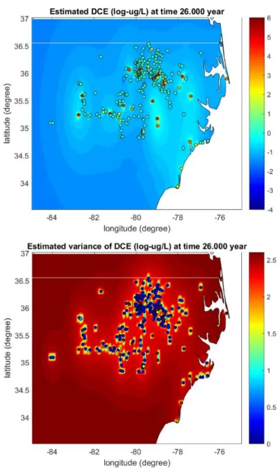
Figure 3: BME Expected Value (a) and Error Variance (b) Map for DCE, 2011
The model aims to have higher expected values around the hard data points with elevated recorded concentrations and then uses the covariance model and simple kriging, where the mean is a constant value of the mean of the hard data points, to estimate the concentration for the entire estimation grid. The reason that there are points with no concentration “islands” around the
19 3.2 Land Use Regression Model
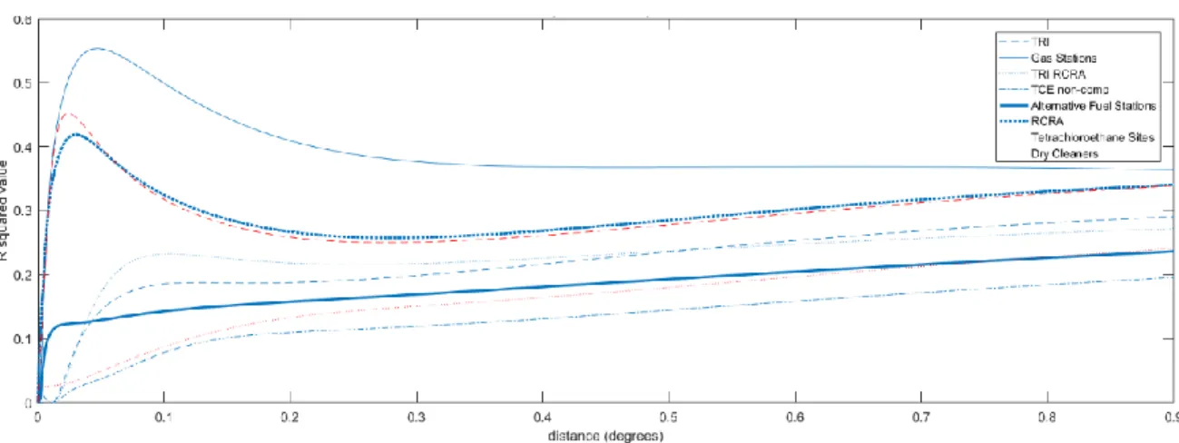
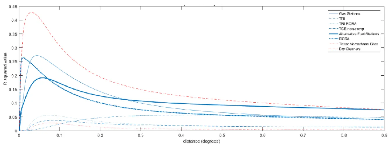
The Land Use Regression results provide some important information in identifying potential sources for contamination of TCE and DCE while confirming the primary source of PCE from previous published studies. We performed an R-squared analysis and comparison for each chemical (PCE, TCE, and DCE) with eight different potential point sources and then
identified the range that produced the highest r-squared value to better analyze which sources are most likely causing the most significant levels of contamination. This has great implications for North Carolina as there is the largest percentage of communities living on private well ground water. Without any previous research studies done on the chemicals TCE and DCE with respect to Land Use in North Carolina, these results can provide informative and substantial information to those who want to test their wells for specific types of chemicals. Having an understanding of the industries surrounding a community will allow future water quality testing to focus on contaminants that are most likely to be released into the water supply.
3.2.1 R-squared Analysis and Optimal Range
The R-squared values and the range at the highest r-squared value are shown in Table 2.
Table 2: Optimal R-Squared Value and Respective Range
DCE TCE PCE DCE Range TCE Range PCE Range TCE Noncompliance Facilities 0.057 7.64E-04 0.1958 0.429 0.069 0.9+ Alternative Fuel Facilities 0.1917 0.0282 0.2365 0.058 0.9+ 0.900
RCRA 0.2646 0.0645 0.4187 0.010 0.007 0.030
TRI RCRA 0.0564 0.0107 0.2716 0.074 0.002 0.9+
Trichloroethane Facilities 0.0279 9.746E-04 0.2409 0.075 0.9+ 0.9+ Dry Cleaners 0.4279 0.3363 0.4517 0.031 0.007 0.024 Gas Stations 0.2717 0.0842 0.5533 0.044 0.025 0.047
TRI sites 0.0376 0.0107 0.2903 0.085 0.002 0.9+
20
DCE’s highest R-squared value of 0.4279 occurred when LUR was performed against dry cleaners at a distance of 3.1km away from each dry cleaner facility. TCE’s highest
R-squared value of 0.3363 occurred when LUR was performed against dry cleaners at a distance of 0.7km away from each dry cleaner facility. PCE’s highest R-squared value of 0.5533 occurred when LUR was performed against gas stations at a distance of 4.7km away from each gas station.
The eight different sources of interest that were analyzed in this study consist of: Toxic Release Inventory (TRI) sites, gas stations, Toxic Release Inventory Resource Conservation and Recovery Act sites (TRI RCRA), TCE non-compliance sites (1990), Alternative fuel stations, Resource Conservation and Recovery Act sites (RCRA), tetrachloroethane sites, and finally dry cleaners. TRI sites are locations that have toxic chemical releases. TRI RCRA sites are
locations that have had hazardous toxic chemical solid waste releases. RCRA sites are locations that have had either a hazardous or non-hazardous solid waste release. These programs are monitored and regulated by the EPA to protect the surrounding communities from
21
Figure 4: R-squared between Tetrachloroethylene and Potential Source Locations
Following Table 2, gas station regression has the highest R-squared maximum value with dry cleaners having second highest, and RCRA sites having the third highest. It is also important to note that the R-squared curve for dry cleaners’ peaks closer to the origin, or at a shorter
distance than the distance to the optimal R-squared for gas stations. Figure 5 shows the R^2 comparison between the potential sources for contamination and TCE.
Figure 5: R-squared between Trichloroethylene and Potential Source Locations
22
Figure 6 shows the R2 comparison between the different potential sources for contamination and DCE.
Figure 6: R-squared between Dichloroethylene and Potential Source Locations
Following Table 2, dry cleaners’ regression has the highest R-squared maximum value with gas stations having second highest, and RCRA sites having the third highest. Note that the R-squared curve for RCRA sites peaks closet to the origin, or at a shorter distance than the distance to the optimal R-squared for Dry Cleaners and Gas Stations.
3.3Land Use Regression Evaluation at Computed Optimal Decay Distance
Land Use Regression plots were created using the optimal r-squared value and
23
Figure 7: LUR estimates Tetrachloroethylene and Dry Cleaner Sites
The small “islands” formed around each of the source locations is indicative of a
functional model. The model is taking the optimal decay distance of 2.4 km for dry cleaners and is estimating the sum of exponentially decaying contributions for each dry cleaner across North Carolina. Higher values are surrounding dry cleaners and gradually reaching a distance where there is a non-concentration or small ambient concentration of PCE. Figure 8 shows the LUR estimate between TCE and RCRA sites.
Figure 8: LUR estimates Trichloroethylene and RCRA Sites
24
tapering off to a zero or ambient value. RCRA was used instead of TRI or TRI RCRA sites because of RCRA’s higher R-squared value and because of the higher R-squared value that was
calculated between DCE and RCRA sites. Figure 9 shows the LUR estimate between DCE and RCRA sites.
Figure 9: LUR estimates Dichloroethylene and RCRA Sites
RCRA sites were again chosen for DCE because of the relatively high R-squared value and the shortest distance of 1km to reach the optimal R-squared value. The “islands” have formed around the RCRA sites and, like PCE and TCE, have tapered off as the distance from each RCRA sites increases.
3.4Criterions Used to Identify Contaminant Sources
25
smaller than a realistic decay distance for TCE and DCE. TCE’s diffusion coefficient is 8.3E-06 and DCE’s is 9.5E-06 sq.cm/sec with their half-lives being respectively 321-1653 days and
56-132 days.20 Therefore, if in the groundwater for three hundred twenty-one days, the diffusion or decay distance is approximately 234 cm or 0.2 meters per year. The increase of the r2 value past the original local peak in the data therefore is not due to the true contamination, but due to large collocational errors with multiple source types falling in between the original point and the longer decay distance.
Additionally, the locational error that occurs with data collection will increase the error margin in this analysis as a geocoded location of a point source may contribute all contamination from a site to the address on the closest street and not in the middle of a land parcel. Because of this, there is an inherent variability of the decay distances which push them to be larger than the expected decay distance of 0.2 meters per year to something closer to 200 meters that we are seeing over longer periods. Dry cleaner sites and RCRA sites are the only two suspected source sites that follow these criteria and therefore are the two sites that will be analyzed in the
26
CHAPTER 4: DISCUSSION
4.1 Comparison of Covariance Ranges and Decay Distances
The chemical TCE degrades into DCE, and it is likely that DCE will have a larger spatial and temporal time lag than TCE because of this degradation. DCE contamination would spread further than TCE because after degrading, DCE will continue to spread out from the source past the TCE contamination. This dispersion acts like a bullseye and the movement from the center rings to the outward rings. Both chemicals have similar time lags in the BME covariance model, TCE with time lags of 10 and 50 years and DCE with time lags of 12 and 60 years. This is very informative when looking at the R-squared analysis and Land Use Regression analysis for both TCE and DCE. Both TCE and DCE have optimal R-squared values at RCRA sites that are very close to the origin, or rather the correlation is highest at a small distance away from the source of pollution.
27
source contamination that the LUR model predicted follows the distribution patterns of TCE and DCE that were documented from the BME analysis.
The similarities between both of these models and prediction strategies lead me to believe that RCRA sites are a source of TCE and DCE contamination, and DCE contamination is in part due to the degradation of TCE. This would explain its slightly larger optimal distance as it spreads over time as well as it’s higher R-squared value as the TCE concentrations may be less
over time as the toxins degrades at these sites.
4.2 Identification of Potential Contamination Sources
The LUR model developed for this analysis successfully reproduces previous studies performed in North Carolina that predicts that dry cleaners are the most accurate predictor source
for PCE because of its high squared value and the smallest distance between the optimal
R-squared and the source of pollutant.3 The distance predicted for the optimal R-squared is likely
greater than that of previous studies because of a more conservative estimation of below detect concentration values in this study and the addition of several years of data. Gas stations'
28
TCE's highest R-squared value is dry cleaners. The optimal decay distance for dry
cleaners is equivalent to the optimal distance TCE had when performing the Land Use
Regression against RCRA sites. This is an indicator that TCE is likely to have several different
sources in North Carolina, with two of them being Dry Cleaners and RCRA sites. TRI and TRI
RCRA sites have the shortest optimal decay distance for TCE, but the R-squared value is so low
that more research would need to be conducted to find a higher correlation. This agrees with the
industries that use TCE in their facilities and would support a more well-defined model if both of
these sources were considered as source contaminant locations. One production source of TCE
is the degradation of PCE and would reach a further decay distance value than that of PCE for
dry cleaners due to the same reasoning as with TCE and DCE.
4.3 Water Quality Current Concerns
With respect to existing policy and room for future growth, there are gaps in the knowledge base for private wells across the country, and especially in North Carolina. There exists a dataset created of 4,314 private wells that had been tested for PCE, TCE, and DCE or a combination of the three.3 This dataset is useful to determine which counties have the highest level of risk for groundwater to contain each of these chemical contaminants. However, of the over 900,000 private groundwater wells that USGS anticipates North Carolina has, only 4,313
private wells were tested for any of the three chemicals studied and only 200,000 wells have ever
been tested for any sort of water quality standards. This means that only 22% of wells in North
Carolina have ever been tested and only 0.46% of wells have been tested for the non-organics
29
Based on other studies, it seems as though the low numbers of sampling for any
contaminants and the even lower numbers for other non-organics testing is common, meaning
that more testing needs to focus on non-organics and metals in water quality panel testing15,16.
This lack of inventory on private well locations is incredibly important and concerning that
private wells exist and are currently not and may have never been tested for contaminants that
surround these communities. In addition to creating an inventory of all private wells in North
Carolina, this study also recommends that water quality sampling schedules should be
encouraged for the protection of public health and reduction of potentially harmful exposure
levels to known carcinogens. The concentration levels that cause chronic cancerous effects from
the Integrated Risk Information System (IRIS) database as well as allowable limits from the
North Carolina Department of Environmental Quality (NCDEQ), work approved 8-hour
exposure limits from the Occupational Safety and Health Administration (OSHA), and the
regulatory maximum allowed concentration in drinking water from the Agency for Toxic
Substances and Disease Registry (ATSDR) can be found in Table 3.
Table 3: Concentration Limits based on Regulation, Health Risks, and Work Safety, 2013
These levels are determined to help protect the public from elevated levels on contamination. If exposed to higher concentration, adverse health effects including chronic
PCE
TCE
DCE
IRIS Chronic Oral RfD (ug/L)
0.006
0.0005
0.02
EPA Chronic Oral (ug/L)
5
5
7
OSHA PEL 8-hour TWA (ug/L)
1000
1000
2000
30
diseases such as cancer and acute illness such as dizziness or even death can occur. After performing analysis on the data, the percentage of sampled points above these values can be found in Table 4.
Table 4: Percentage of Samples Greater than Allowable Limit, 2013
Having percentages of levels higher than the recommended limits for TCE thirty-eight percent of the time is concerning and needs to be addressed immediately. People of North Carolina are being exposed to elevated levels of contamination where they work and at home. They are consuming contaminated water and all three chemicals have been proven through this sample analysis to be present in groundwater. PCE and TCE according to the EPA and IRIS have goal concentrations of zero parts per billion. With as high as thirty-eight percent of the close to ten-thousand TCE data points being greater than the chronic oral exposure dosage, there is a lot of work to be done to improve the safety of drinking water.
Although zero parts per billion for PCE and TCE contamination are a long-term goal, to better understand what regions in North Carolina should test their wells for the three different
contaminants, several maps were created that show in red the locations where testing should be
performed, using the EPA’s chronic oral levels of contamination as a cut-off to where this testing
should be required. For each of the three chemicals- DCE, TCE, and PCE- a map was created
for each exposure from RCRA sites and from Dry Cleaner sites. The different contamination
PCE
TCE
DCE
% above chronic IRIS level
18.22%
38.24%
17.48%
% above chronic EPA level
7.56%
23.04%
4.48%
% above chronic OSHA level
1.23%
5.06%
0.10%
31
sites were intentionally mapped separately and not combined as to preserve the variation in
contamination sources from each of the two. This is especially important due to the discrepancy
between the levels of contamination of TCE from dry cleaner sites and the assumption that a
majority of the TCE contamination from Dry Cleaner sites is due to the degradation of PCE into
TCE. These maps in figure 10 a-f (DCE, TCE, PCE) show locations where testing should be
required to prevent further consumption of these contaminants through private well water.
a.
32 c.
d.
33 f.
Figure 10 (a-f): Contamination levels about the EPA Allowable Drinking Limit (log ug/L), 2013
The same range of values was used for each chemical to easily compare the exposures from RCRA sites and Dry Cleaners. Levels of all chemicals are seen around major metropolitan areas- such as Charlotte and the Research Triangle. However, there are variations in the
exposures if the RCRA and Dry Cleaner maps are compared, which supports the hypothesis that exposure comes from both of these sources and should have their own policies and regulations.
Furthermore, it is important to consider the population density of private well consumers when looking at these maps. These areas should all be tested as they have levels of
34
Figure 11: Residents Using Private Wells Normalized by Population Density/County, 2010
The data was normalized by population density to reduce the influence that city
populations would have on the numbers aggregated by the percentages of consumers on private well water. This enables the estimate to be a more accurate representation of the actual values of people on private wells per county in North Carolina.
35
CHAPTER 5: CONCLUSION
In summary, using BME, as well as LUR is useful in determining the primary source of contamination for a specific chemical. Being able to compare covariance plots and LUR
analyses allowed us to conclude that RCRA sites are possible sources of TCE and DCE pollution at short distances.
PCE contamination in North Carolina appears to have sources primarily in Dry Cleaner sites. TCE contamination in North Carolina has the potential to come from TRI and TRI RCRA facilities, but more than likely has pollution streams from dry cleaners and the degradation of PCE to TCE as well as RCRA sites and the degradation from TCE to DCE. DCE contamination appears to have sources primarily from dry cleaners and RCRA sites. Gas stations were
eliminated as an option of contamination based on the fact that the optimal r-Squared between contaminant and source location and the distance to reach the optimal decay distance was too high to feasibly be a direct source of groundwater contamination for PCE, TCE, and DCE.
From this research, it can be concluded that policy decision makers need to reevaluate the lack of policy provided to protect private well owners from contamination in their wells.
Currently there is no policy in place for regular sampling of wells. There is a likely chance that a large percentage of North Carolina’s residents are being exposed to, and suffering from health
36
regulations. Additionally, with TCE and PCE’s association with renal cancer and other chronic diseases and TCE’s designation as a known carcinogen, these policy changes should be put on
the priority list as a major public health concern for the people of North Carolina.
5.1 Future Steps and Policy Recommendations
These results will help communities narrow down which contaminants of interest they should test for in their private wells as they can focus on industrial facilities surrounding their communities to see whether they may be at-risk for high concentrations of PCE, TCE, or DCE. Additionally, the model developed to create the analysis in this study is easily amendable to include any other source dataset with latitude and longitude locations and can provide
communities without resources the ability to quickly predict spatially where contaminant plumes will impact the community. Additional inventories should be taken to determine the spatial locations of private wells in North Carolina, as the current available data is lacking and hinders the investigation of the effects of contaminants and protection of private well users.
37
around suspected contamination sites, which hinders the analysis on determining what is being polluted at these sources. A recommendation would be to improve the inventory of these contamination sites as they are already designated by the EPA as locations of concern. For example, RCRA sites are designated by the EPA as sources of either hazardous or non-hazardous contamination. Therefore, it would be a simple policy recommendation to require sampling surrounding these sites and not just understanding the geographic location of these sites would be a positive step forward in addressing these areas of concern. Dry Cleaner remediation has been so successful due to the Dry Cleaner Solvent Clean Up Act (DSCA) which stipulates a focused effort of testing at and around dry-cleaning sites for known volatile organic compounds, and the focused effort in sampling at and around dry cleaners to determine the contamination coming from dry cleaners. This same model should be implemented for RCRA sites as well as other known regulated sites to determine what type of contamination is coming from which sources.
38
public water. Finally, North Carolina should review its allowable levels of contaminants and adjust their allowable limits to match with IRIS levels to better protect the residents. Because as it stands, North Carolina’s limits are sometimes one- hundred times higher than that of IRIS
levels. Of course, there is a balance that needs to be found between reducing allowable limits and feasibility, but it is certain that North Carolina needs to take steps towards protecting its private well users more so than they currently are.
39
APPENDIX: SUPPLEMENTARY INFORMATION
Chemical Background Information:
1. Tetrachloroethylene
Tetrachloroethylene or PCE is a hydrophilic chemical that has been used historically for chemical intermediates - 55%, metal cleaning and vapor degreasing - 25%, dry cleaning and textile processing - 15%, and other unspecified uses - 5%. It is a Clear, colorless, nonflammable liquid with a sweet, fruity odor like that of chloroform. According to the EPA, PCE is considered likely a carcinogen and will be looked at again through the next round of toxicity analyses. PCE has been linked to renal cancer and has the potential to cause further chronic and acute illnesses
2. Trichloroethylene
Trichloroethylene or TCE is a hydrophilic chemical that has been used historically for Vapor degreasing of fabricated metal parts in the automotive and metal industries – 80% as well as in consumer products that contain TCE include: Adhesives, Spot removers, Cleaning fluids for rugs, Paint removers/strippers, and Typewriter correction fluids. It is a common industrial solvent and contaminant of hazardous waste sites, groundwater, and drinking water. TCE according to the EPA is considered to be a known carcinogen and has been linked to liver cancer, renal cancer, and kidney cancer, as well as some blood cancers.
3. Dichloroethylene
40
volatile organic compound that is highly flammable, colorless liquid with a sharp, harsh odor. DCE according to the EPA is not considered a carcinogen or a likely carcinogen, but due to the association between DCE and TCE and PCE, it is likely that this will be relooked at in the next round of toxicity analyses.
PCE, TCE, and DCE Data sources:
Messier et. Al 2012 provides information on the acquisition of data for his PCE analysis:
“Data on groundwater PCE were compiled from three sources, which are detailed as follows: North
41
of Transportation line reference, then with a U.S. street address line reference file. All geocoded addresses with a match score of 70 and above were included in the data set. The address geocoding resulted in 2411 geocoded wells with 2874 space/ time samples (out of 4102) from the years 2003−2010 that were previously unavailable. We downloaded all of the PCE well data available from the USGS NWIS Web site. We obtained 71 monitoring wells”3
TCE and DCE datasets were created replicating his methods for PCE using the same databases he had used to improve the existing dataset and include more recent data points- bringing the dates of analysis through 2015. PCE’s DSCA database increased in size mostly due to the increase of samples that did not exist when Messier’s paper was published Table S1 shows the hard datasets that were used in
this analysis
Table S1: Hard datasets Created for Analysis
DSCA USGS Private Wells Total
PCE unique 125 215 1160 1500
PCE space-time 7464 343 1408 9215
TCE unique 124 226 1162 1512
TCE space-time 7277 357 1421 9055
DCE unique 862 20 1009 1888
42
43 REFERENCES
1. Agency for Toxic Substances and Disease Registry Case Studies in Environmental Medicine (CSEM)
Trichloroethylene Toxicity. (2018). [ebook] U.S. Department of Health and Human Services Agency for Toxic Substances and Disease Registry Division of Toxicology and Environmental Medicine Environmental Medicine and Educational Services Branch. Available at:
https://www.atsdr.cdc.gov/csem/tce/docs/tce.pdf
2. Eckhardt, David AV, William J. Flipse, and Edward T. Oaksford. Relation between land use and
ground-water quality in the upper glacial aquifer in Nassau and Suffolk Counties, Long Island, New York. Vol. 86. No. 4142. Department of the Interior, US Geological Survey, 1989.
3. Messier, Kyle P., Yasuyuki Akita, and Marc L. Serre. "Integrating address geocoding, land use regression, and spatiotemporal geostatistical estimation for groundwater tetrachloroethylene." Environmental science & technology 46.5 (2012): 2772-2780.
4. Pubchem.ncbi.nlm.nih.gov. (2018). 1,2-Dichloroethylene. [online] Available at:
https://pubchem.ncbi.nlm.nih.gov/compound/trans-1_2-dichloroethylene#section=Top
5. United States Geological Survey. National Water Information System. http://nwis.waterdata.usgs.gov
6. Akita, Y.; Carter, G.; Serre, M. L. Spatiotemporal Nonattainment assessment of surface water
tetrachloroethylene in New Jersey. Environ Qual. 2007, 36, 508−520.
7. Puangthongthub, S.; Wangwongwatana, S.; Kamens, R.; Serre, M.L. Modeling the space/time
distribution of particulate matter in Thailand and optimizing its monitoring network. Atmos. Environ. 2007,41, 7788−7805.
8. De Nazelle, A.; Arunachalam, S.; Serre, M. L. Bayesian maximum entropy integration of ozone
observations and model predictions: An application for attainment demonstration in North Carolina. Environ. Sci. Technol. 2010, 44 (15), 5707−5713.
9. Christakos, G. A Bayesian/maximum-entropy view to the spatial estimation problem. Math. Geosci.
1990, 22 (7), 763−776.
10. NCOnemap. Geographic Data Serving A Statewide Community. http://www.nconemap.com/
11. Ncdenr.maps.arcgis.com. (2018). [online] https://ncdenr.maps.arcgis.com/home/index.html
12. National Center for Biotechnology Information. PubChem Compound Database; CID=31373,
https://pubchem.ncbi.nlm.nih.gov/compound/31373
13. National Center for Biotechnology Information. PubChem Compound Database; CID=6575,
https://pubchem.ncbi.nlm.nih.gov/compound/6575
14. Environmental Protection Agency. https://www.usepa.com/privatewells
15. Permitting and Inspection of Private Drinking Water Wells. NCAC 02C .0301 Scope and Purpose.
https://ehs.ncpublichealth.com/owsp/docs/
16. Wartenberg, D, D Reyner, and C S Scott. “Trichloroethylene and Cancer: Epidemiologic Evidence.”
44
17. U.S. Geological Survey. 2016. ”Water Use Data for North Carolina.“
https://waterdata.usgs.gov/nc/nwis/wu.
18. “Resource Conservation and Recovery Act (RCRA) Laws and Regulations.” EPA, Environmental
Protection Agency, 6 Feb. 2018, www.epa.gov/rcra.
19. “Resource Conservation and Recovery Act (RCRA) Laws and Regulations.” EPA, Environmental
Protection Agency, 6 Feb. 2018, www.epa.gov/rcra.
20. “Top Eight Alternative Fuels.” CleanTechnica, 17 June 2013,
cleantechnica.com/2012/03/08/top-eight-alternative-fuels/.
21. “Contaminant Fate and Transport.” EPA, Environmental Protection Agency, 19 March 2018,