Bost_unc_0153M_16053.pdf

HOW STORMS AFFECT CARBON BURIAL IN THE NEW RIVER ESTUARY, NORTH CAROLINA

Molly Chapin Bost

A thesis submitted to the faculty at the University of North Carolina at Chapel Hill in partial fulfillment of the requirements for the degree of Master of Science in the Department of Marine Sciences

Chapel Hill 2016

ABSTRACT

MOLLY CHAPIN BOST: HOW STORMS AFFECT CARBON BURIAL IN THE NEW RIVER ESTUARY, NORTH CAROLINA

(Under the direction of Brent A. McKee)

Estuaries provide many ecosystem services, but one that is not well quantified is carbon burial. The New River Estuary (NRE) is a wave dominated, multi-lagoon system with limited connectivity to the ocean. The goal of this study is to assess changes in carbon burial rates over the past century within the NRE. The NRE has undergone changes including development of a Marine Corps base, eutrophication followed by remediation, and hurricanes, all of which affect carbon burial rates. Mean sediment

ACKNOWLEDGEMENTS

First and foremost, I must express my sincerest gratitude to my advisor, Brent McKee. While bearing many responsibilities in the Marine Sciences department, he has never been anything but supportive, patient, and accessible. His enthusiasm for this project and having me as his student has provided me with fuel throughout my thesis work. I cannot imagine a better advisor.

Thank you to my committee members, Dr. Jaye Cable and Dr. Tony Rodriguez who helped balance my research by providing perspective and bringing a depth to my work that I wouldn’t have otherwise.

I could not have finished my laboratory analysis in a timely manner if it weren’t for a small army of undergraduates lead by John Gunnel who orchestrated the initial processing of my samples. Thank you also to Sherif Ghobrial for helping to troubleshoot the many sudden and unexpected issues that inevitably arise in an acid lab.

I appreciate the time and effort spent by Dr. Anna Jalowska who taught me the long and laborious alpha procedure. Her continued support and help throughout my work has been a keystone to my success. Due to her guidance, I now read the alpha procedure in a Polish-American accent.

Thank you to the entire DCERP team for affording me the great opportunity of being part of an amazing communal effort to create a carbon budget in the New River Estuary. Notably, thank you to Craig Tobias and Bryce Van Dam for sharing data willingly to help with my final analyses.

Thank you to my cohort for their fierce support, feedback, and friendship. Most especially, thanks to my great friend, Jill Arriola. In the three years I’ve had the pleasure of knowing Jill, I have come to know her as an inspiring person and an extraordinary friend. I would not have survived graduate school without her unwavering encouragement and friendship.

TABLE OF CONTENTS

LIST OF TABLES………...vii

LIST OF FIGURES………viii

LIST OF ABBREVIATIONS………...ix

1. INTRODUCTION……….1

2. SEDIMENTATION AND CARBON BURIAL IN ESTUARIES………...2

3. USING 210Pb TO DETERMINE SEDIMENT ACCUMULATION AND CARBON BURIAL RATES……….4

4. SITE DESCRIPTION………..5

5. METHODS………7

5.1 Core Collection………7

5.2 Porosity and Dry Bulk Density………..8

5.3 210Pb Determination via Alpha Spectrometry……….8

5.4 Modeling………...9

5.4.1 Constant Rate of Supply (CRS) ………..10

5.4.2 Constant Initial Concentration (CIC) ………...11

5.4.3 Constant Flux Constant Sedimentation (CFCS) ………...11

5.5 Carbon Burial Rates……….12

6. RESULTS………...13

6.1 210Pb Profiles………...13

6.2 Modeling……….14

6.3 Total Core Inventories………..15

6.4 Sediment Accumulation Rates (SAR)………16

6.5 Mass Accumulation Rates (MAR)………..17

6.6 Drivers of Carbon Burial Rates………...18

7. DISCUSSION……….20

7.2 Total Inventories………20

7.3 Mass and Sediment Accumulation Rates……….21

7.5 Carbon Burial Rates……….22

8. CONCLUSION………..……….24

APPENDIX 1. PLOTS FROM NRE-1 AND NRE-3………...………...25

APPENDIX 2. COMPARISON TO OTHER MODELS………33

LIST OF TABLES

Table

LIST OF FIGURES

Figure

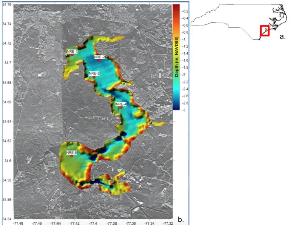
1. Bathymetric map of study site………...7

a. Map of North Carolina………..………...7

b. NRE bathymetry map with coring locations of usable geochronologies………7

2. 210Pb profiles for NRE-2, NRE-4, and NRE-6……….13

3. Sediment accumulation rates of NRE-2, NRE-4, and NRE-6………..16

4. Mass accumulation rates of NRE-2, NRE-4, and NRE-6………...17

LIST OF ABBREVIATIONS

CAFOs Concentrated Animal Feeding Operations CFCS Constant Flux Constant Sedimentation CIC Constant Initial Concentration

CRS Constant Rate of Supply ICW Intracoastal Waterway MAR Mass Accumulation Rates

MCBCL Marine Corps Base Camp Lejeune NC North Carolina

1. INTRODUCTION

Estuarine systems are ubiquitous and, because of their many services, they have supported the growth and development of the communities surrounding them. Of the 32 largest cities in the world, 22 are located on estuaries (NOAA’s National Ocean Service Education: Estuaries, 2011). Land use change, accelerated rates of relative sea-level rise, and changing intensities and frequencies of hurricanes pose threats to estuarine systems and the ecosystem services they provide. Some of these ecosystem services include providing a nursery habitat to valuable fishery species, buffering against storm surges, filtering pollutants out of the water column, and burying carbon. The carbon sequestration and burial potential in estuaries is poorly constrained and not well understood. This study examines the human and climate factors that impact sedimentation and carbon burial rates within the New River Estuary, North Carolina.

The primary research questions for this study were as follows:

1. How have sedimentation and carbon burial rates changed over the last 100-150 years? 2. What are the drivers of carbon burial in the New River Estuary?

2. SEDIMENTATION AND CARBON BURIAL IN ESTUARIES

A recent phenomenon in Carbon budgeting on a global scale has been attributing a color code to the carbon buried in marine and terrestrial environments. Green carbon is associated with the carbon buried in terrestrial environments and blue carbon is buried in marine environments including tidal salt marshes, mangroves, and sea grasses (Mcleod et al, 2011). Since the carbon entering an estuary could be from terrestrial sources or marine sources, it is difficult to distinguish into which category estuarine carbon fits.

There have been inconsistencies in the literature associated with the terminology defining the fate of carbon in these blue carbon environments. This study proposes the following definitions:

1. Carbon burial: Rates associated with the processes of diagenesis that occur within the top few centimeters of the sediment on an annual timescale.

2. Carbon sequestration: A measure of total carbon in the entire ecosystem including living biomass, above and belowground biomass, carbon in the sediments, but not carbon in the atmosphere. This could range on timescales of days to millennia.

3. Carbon storage: The amount of carbon that is locked in the sediments below zones of early diagenesis (>1m) on timescales of decades to millennia.

challenging because of the dynamic processes affecting carbon source, sedimentation, and preservation of organic carbon.

The balance between sediment supply, accommodation space, and energy dictates

sedimentation in an estuary (Zhu and Olsen, 2013). The accommodation space in an estuary is a function of the changes in relative sea-level and the morphology of the basin (Mattheus and Rodriguez, 2010). On a passive margin, like the Eastern United States, at low stands of sea level, valleys are incised and as sea level rises, accommodation space increases. The sediments in wave and tide dominated (Dalrymple et al, 1992) estuaries are constantly reworked through erosion and deposition, which results in disturbed sediment records. Constructing high-resolution records of estuarine sedimentation and linking measured changes in accumulation rate to a change in carbon burial is an important step toward predicting the response of estuaries to human (land-use changes) and climate (accelerating sea level rise and changes in storm frequency and intensity) impacts.

Little is known about how tropical storms affect carbon burial in estuaries Hurricanes can alter the sediment flux to estuaries by altering the supply from riverine and marine environments, from shoreline erosion, and by remobilizing previously deposited sediments (Elliot et al, 2015). One tool for

3. USING 210Pb TO DETERMINE SEDIMENT ACCUMULATION AND CARBON BURIAL RATES

Much of the coastal development in North America has occurred in the last 100-150 years, making 210Pb the ideal isotope to study in these systems surrounded by change. 210Pb has a half-life of 22.3 years (“Western Lake Catchment Systems”) and is a naturally-occurring radioisotope that is part of the Uranium-238 (238U) decay series. 238U decays to Radium-226 (226Ra), which is found at low and relatively consistent concentrations in sediments around the world. 226Ra decays into Radon-222 (222Rn), which can either remain in the sediments or escape into the atmosphere. In either scenario, 222Rn decays into 210Pb, but the 210Pb that occurs in the sediment decay of 222Rn is termed “supported”. “Unsupported” or excess (XS) 210Pb occurs from the 222Rn that decays in the atmosphere, falls out, and adsorbs to particles that then settle into the sedimentary record (Appleby and Oldfield, 1983).

The analysis of 210Pb geochronologies depends heavily on the validation of the models used. There are several geochronology models that operate under a number of different assumptions. The Constant Initial Concentration, Constant Rate of Supply, and Constant Flux: Constant Sedimentation models are discussed in section 5.4 and were used to analyze the data presented here. It has become increasingly clear in the literature that these models cannot be applied to every estuarine, lacustrine, or marine system. The best approach, according to Appleby 2002, has been to apply each of these models to the data and compare them while also using a validation techniques either with other

chronostratigraphic tracers either from the fallout of non-naturally occurring radioisotopes like 137Cs or 14C or, as is demonstrated in this research, by comparing the dates to other major events like hurricanes.

4. SITE DESCRIPTION

The New River is a 5th order black water stream located in Onslow County in Eastern North Carolina. The river empties into a choked lagoon estuarine system with four practically separate lagoons between the head and mouth of the estuary. According to the Dalrymple 1992 characterizations of estuaries, the New River Estuary can be classified as a wave dominated coastal plain estuary formed on a drowned river mouth. This morphology suggests that the New River Estuary currently has the most

accommodation space in its history since it was incised during the last glacial maximum. Jacksonville, NC is oriented at the head of the estuary and Marine Corps Base Camp Lejeune (MCBCL) surrounds it to the East and West. The mouth of the estuary is restricted by a barrier island system, causing the estuary to be microtidal and have a very long flushing time of 64 days (Mallin et al, 2005). Choked lagoons are relatively disconnected from ocean as well as the other small lagoons within the system, which

contributes to the tide and salinity ranges; mesohaline to polyhaline (Dame et al, 2000). The estuary is approximately 80 km long; 3 km wide, and over half of the estuary is less than two meters deep making it a relatively small and shallow system. MCBCL uses the NRE to perform amphibious military training so it is frequently dredged to maintain channels including the Intracoastal Waterway (ICW), which was built in about 1936 (“Background- History”), near the mouth of the estuary.

greatly improved the water quality in the New River Estuary and reduced labile carbon from phytoplankton.

Since 1851, 103 hurricanes and tropical storms have directly or indirectly impacted the study area for this project, Onslow County in North Carolina (“Hurricanes”). In 1999, two of the most impactful storms since the 1940s made landfall in North Carolina only twelve days apart. Dennis made landfall on

September 4th, 1999 in North Carolina as a Tropical Storm. Dennis had an unusually erratic path, moving along the NC coast, but then circulating back around to make landfall just North of the NRE at Cape Lookout. This prolonged the duration of impact, maintaining the above normal tides longer than usual. Rainfall estimates from Dennis range from 6-10 inches, which set the stage for Hurricane Floyd (“Tropical Storm Dennis), which came ashore on September 16th as a category 2 hurricane with wind speeds of about 177 kph and storm surge of about 2.5 meters (“Hurricane Floyd”). Floyd brought significant rainfall but without Dennis having saturated Eastern North Carolina, such intense flooding throughout the region likely wouldn’t have been as severe. The record rainfall caused a major increase in nutrient loading from the swine CAFOs and increased sediment loads. These severe storms and their effect on sedimentation and carbon burial rates are of great interest in this study.

To investigate a carbon budget, the estuary was divided into upper, middle, and lower estuary. Three sediment cores were taken in the upper, two in the middle estuary and two in the lower estuary for a total of seven cores. Each coring location was chosen based on previous grab samples indicating a muddy bottom, similar depths, and the assumption that 210Pb deposition would be similar to atmospheric values of 0.827 dpm cm-2 yr-1 (Benninger and Wells, 1993). Cores were named NRE-1, 2, 3, 4, 5, 6, and 7 moving from the head to the mouth of the estuary. Five of the seven cores yielded usable

a. 5. METHODS

5.1Core Collection

Fifty-centimeter cores were taken using aluminum core tubes with a 10-centimeter diameter. Cores were taken by hand using a coring device with a one-way valve to retain the sediments and an extension rod to access deeper water depths. Each core was subsampled into one-centimeter intervals and placed into appropriately labeled plastic bags. The first five centimeters of each core and every other interval after 5 cm were divided approximately in half for further laboratory analysis including Carbon to Nitrogen ratios and percent organic carbon.

Figure 1. a. North Carolina map with NRE indicated by red box. b. Bathymetry map from NAVD88 shows coring locations of sites with reported data indicated by red dots.

b.

5.2 Porosity and Dry Bulk Density

Porosity and dry bulk density were calculated for each interval using measurements of weight before and after the sample was lyophilized in a freeze drier. Samples were then pulverized and sieved. Portions larger than 2mm are considered “extra”, fractions between 2 mm and 500 micrometers are considered “coarse”, and portions less than 500 micrometers are considered “fine”. Fine fractions were used for alpha spectrometry described in the next section.

5.3 210Pb Determination via Alpha Spectrometry

Excess (XS)210Pb activities were determined via isotope-dilution alpha spectrometry for the granddaughter isotope, 210Po, which is in secular equilibrium with 210Pb. A detailed methodology is presented here because it combines and modifies methods used previously.

210_{Po is a naturally occurring α-emitter with a half-life of 128.4 days (NuDat2.6, 2012).} 210_{Po is a}

product of decay within the 238U series as a decay product of 210Pb. 210Pb activities were determined via isotope-dilution alpha spectrometry for the 210Pb granddaughter isotope 210Po, which are in secular equilibrium with each other ( Flynn, 1968; Matthews et al., 2007).

Fine fraction of sediment was packed into Teflon vessels, 1.4-1.6 g each. Each sample was spiked with 1.0ml (~20dpm) 209Po tracer (Oak Ridge National Laboratories) diluted in 1M Certified ACS Plus hydrochloric acid and 15ml of Certified ACS plus 15M nitric acid (Smitth-Briggs et al., 1986; Bradley, 1993).

3500 rpm for 8 minutes. The supernate was combined with the rest of the leached samples in the Teflon beakers on the hot plate. The remaining sediment was discarded. Temperature of the hot plate was kept between 85-90°C, not to exceed 95°C to avoid losses due to volatilization of the 209Po tracer (Martin and Blanchard, 1969). When the solution in the beakers had warmed up, 1-2ml of 10.3M hydrogen peroxide was titrated to each beaker to let effervesce. Addition of hydrogen peroxide (Jia et al., 2004) releases organic components not destroyed by heating with nitric acid as carbon dioxide (Martin and Hancock, 2004). Nearly dried samples were then dissolved in 15ml DI water. In the next step, samples were titrated with ammonium hydroxide to raise the pH to 7-8.5. Change in pH allowed iron precipitation. Precipitated iron was collected via centrifugation for 8 minutes at 3500 rpm and then rinsed twice with 30ml of DI water. The iron precipitate was then dissolved with 3.75ml 10M Certified ACS Plus hydrochloric acid and treated with ~50-60 mg of ascorbic acid to eliminate the interference of iron by reducing it to the ferrous state, Fe3+ to Fe2+ (Blanchard, 1966). Samples were transferred back to Teflon beakers with labeled stainless steel disks called planchets and stir bars. The planchets are coated with foil on one side. To assure maximum yields, samples were allowed spontaneous deposition for 20-40 hours with stirrers at 200-300 rpm at room temperature. The next day the planchets were removed from solution, rinsed with DI water and left to air dry for 24 hours. The planchets were then transferred to α -particle spectrometry utilizing Passivated Implanted Planar Silicon (PIPS®) detector for counting for 24 hours.

5.4 Modeling

5.4.1 Constant Rate of Supply (CRS)

The CRS model is rooted in the assumption that unsupported 210Pb flux to the sediment surface is constant, but initial concentrations of 210Pb in each layer and sedimentation rates throughout the core can vary. As the mass accumulation rates and initial concentrations in each layer change, they must be inversely proportional so

Constant

Where C0 is the initial activity and rt is the mass accumulation rate (g cm-2 yr-1)

To get a total inventory of cumulative excess 210Pb in the core:

Where Ax is the cumulative excess 210Pb in the core beneath a depth z and A0 is the cumulative excess

210_{Pb activity in the sediment core beneath the sediment-water interface.}

The sedimentation rates using the CRS model were calculated using the following formula.

𝑟

=

!!! !

where r is the sedimentation rate, λ is the decay constant, Ax is the cumulative excess 210Pb beneath

depth z, and C is activity.

C

₀

×

r

_t

=

5.4.2 Constant Initial Concentration (CIC)

The Constant Initial Concentration (CIC) model assumes that there is a constant initial concentration of 226Ra, a constant specific activity of 210Pb, and a constant sedimentation rate. This is described by the formula below.

Where CTx is the total 210Pb at uncompacted depth x and age t. C0 is the excess 210Pb at the

sediment-water interface. C* is the supported level of 226Ra and is the decay variable given the decay

constant, , and time t. This model assumes that the ratio of the flux of 210Pb to the sediment-water

interface (P) to the mass accumulation rate (r) is constant. This is shown by the formula below.

In order to get time in the past (t), divide the centimeter interval (x) by the Sedimentation rate (S0)

described by the formula below.

5.4.3 Constant Flux Constant Sedimentation (CFCS)

The Constant Flux Constant Sedimentation model is a piece-wise CRS model. The primary assumptions are: constant 210Pb flux to the sediment surface, constant mass accumulation rate, and that 210_{Pb concentrations, when a layer is formed, is constant so mass accumulation, which can vary, is}

inversely proportional to 210Pb flux to the sediment surface

Where Ciis the excess 210Pb concentration in layer i, f is the excess 210Pb flux to the sediment surface,

and r is the mass accumulation rate. This model allows for the interpretation of data in a piece-wise fashion.

C

T

x

=

(

C

0

)

e

−λt

+

C

*

e

−λt

λ

C

₀

=

P

r

t

=

x

S

0

C

i

(

t

=

0)

=

5.5 Carbon Burial Rates

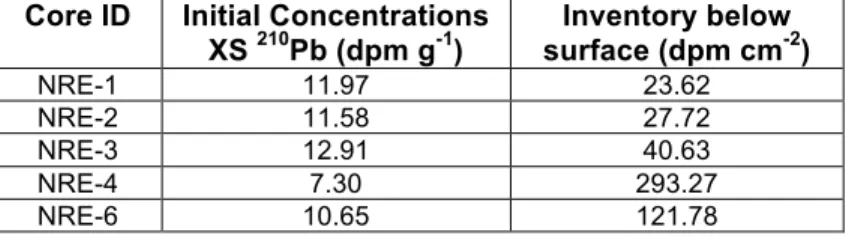
Figure 2. 210Pb profiles for NRE-2, NRE-4, and NRE-6 6. RESULTS

6.1 210Pb profiles

Figure 2 shows the XS 210Pb profiles for NRE-2, NRE-4, and NRE-6. NRE-1 and NRE-3 are presented in Appendix 1. NRE-1, 2, and 3 are all very similar profiles so NRE-2 was chosen to represent the upper estuary cores. XS 210Pb is plotted against mass depth with XS 210Pb on the x-axis in dpm g-1. The 210Pb profile of NRE-2 is representative of the exponential decay of 210Pb in the sediments. NRE-4 has a mass depth axis more than three times that of NRE-2 and NRE-6 and a nomonotonous XS 210Pb profile indicating frequent disturbance and higher sedimentation in this part of the estuary. The XS 210Pb profile at NRE-6 deviates from the curve in a more consistent pattern indicating some disturbance, but not as much as NRE-4.

0.0 0.5 1.0 1.5 2.0 2.5 3.0 3.5

0 2 4 6 8 10 12 14

mi

(g cm-2)

NRE-2

_210Pb

ex (dpm g-1)

0 2 4 6 8 10 12 14

0 2 4 6 8 10 12 14

mi

(g cm-2)

NRE-4

₂₁₀

Pbex (dpm g-1)

0 0.5 1 1.5 2 2.5 3 3.5 4

0 2 4 6 8 10 12 14

mi

(g cm-2)

NRE-6

210_Pb

6.2 Modeling

The application of all three geochronology models (CIC, CRS, and CFCS) was pertinent to the correct interpretation of data from the New River Estuary cores. The CIC and CFCS models would work relatively well for the upper estuary cores since their profiles followed the exponential curve. However, given the discontinuity of the middle and lower estuary XS 210Pb profiles, the CIC and CFCS models would not work for the entire system. Nonmonotonous XS 210Pb profiles indicate episodic deposition or erosion of the sedimentary record.

Given the variable sediment accumulate rates in the XS 210Pb profiles and the confirmation of dates compared to hurricane events in 1999, the CRS model proved most valid for this data set. The CIC and CFCS models calculated much lower mass accumulation rate than the CRS model likely because those models average rates over the entire profile without taking peaks into consideration. According to the CRS model, MAR varied over time in the NRE, which invalidates the CIC and CFCS models.

6.3 Total Core Inventories

According to Benninger and Wells (1993), North Carolina 210Pb inventories supported by atmospheric flux only are approximately 26.52 dpm cm-2. NRE-1 had a total inventory of 23.62 dpm cm-2 which is slightly lower than the quoted average for the region. The rest of the cores in the upper estuary had higher inventories than average for the region. NRE-2 had only slightly higher at 27.72 dpm cm-2, while NRE-3 had almost twice the average with 40.63 dpm cm-2. In the middle estuary, NRE-4 had the highest inventory of 293.27 dpm cm-2, about 11 times higher than average. NRE-6, the most seaward core had 121.78 dpm cm-2, almost five times the inventory of average values. The initial concentrations of excess 210Pb at NRE-1 and NRE-2 and NRE-3 were all relatively similar at 11.97 dpm g-1, 11.58 dpm g -1_{, and 12.91 dpm g}-1 _{respectively. NRE-4 had the lowest initial excess} 210_{Pb concentration of 7.30 dpm g} -1_{and NRE-6 had still slightly lower initial concentrations of 10.65 dpm g}-1_.

Core ID Initial Concentrations XS 210Pb (dpm g-1)

Inventory below surface (dpm cm-2)

NRE-1 11.97 23.62

NRE-2 11.58 27.72

NRE-3 12.91 40.63

NRE-4 7.30 293.27

NRE-6 10.65 121.78

1865 1875 1885 1895 1905 1915 1925 1935 1945 1955 1965 1975 1985 1995 2005 2015

0.00 0.50 1.00 1.50

SAR (cm yr-1)

NRE-2 1865 1875 1885 1895 1905 1915 1925 1935 1945 1955 1965 1975 1985 1995 2005 2015

0.00 2.00 4.00 6.00

SAR (cm yr-1)

NRE-4

1865 1875 1885 1895 1905 1915 1925 1935 1945 1955 1965 1975 1985 1995 2005 2015

0.00 SAR (cm yr-1) 2.00 4.00

NRE-6

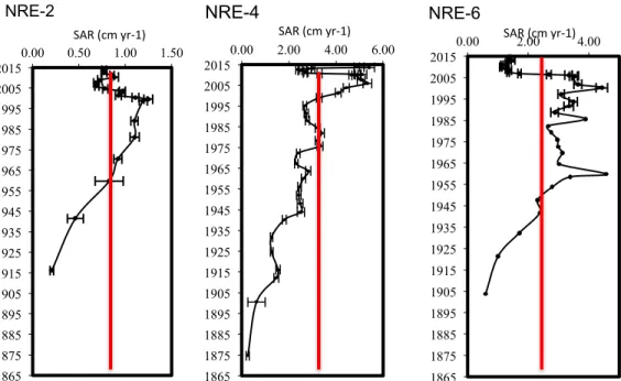
6.4 Sediment Accumulation Rate (SAR)

Based on the CRS model, NRE-1, NRE-2, and NRE-3 have similar average SAR values (0.71, 0.86, 0.74 cm yr-1 respectively). The plots for NRE-1 and NRE-3 are shown in Appendix A. The average SAR at NRE-4 and NRE-6 are much higher (3.02 cm yr-1 2.50 cm yr-1 respectively). All of the cores have a peak in sediment accumulation rates in 1999 followed by a period of much lower rates. NRE-6 has multiple distinct peaks including one in 1999. SAR in all cores began to return to values similar to those prior to the 1999 peak around 2008. The SAR for all cores ranges from two to ten times the estimated rate of local RSLR; NOAA estimates that RSLR in North Carolina is between 0-3 mm yr-1 or 0-.3 cm yr-1. Rates of sediment accumulation in the New River Estuary are much higher than that of local sea level rise, but these coring locations were selectively chosen because of their likelihood to be depositional areas in the estuary so these results may be on the high end of those found in the NRE. The plots in Figure 3 use the CRS model to determine sediment accumulation rates since 1865.

0.0 0.5 1.0 1.5 2.0

MAR (g cm-2 _yr-1₎

NRE-6

2000.2

1985.6

1959.82

0.0 0.1 0.2 0.3

MAR (g cm-2 _yr-1₎

NRE-2

1998.85

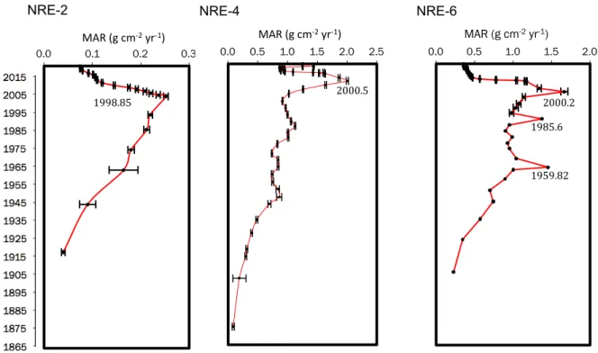
Figure 4. Mass accumulation rates of NRE-2, NRE-4, and NRE-6. Dates associated with each peak are indicated next to the peak

0.0 0.5 1.0 1.5 2.0 2.5

MAR (g cm-2 _yr-1₎

NRE-4

2000.5

6.5 Mass Accumulation rates

Mass accumulation rates over time showed a steady increase since the late 1800s with peaks in the late 1990s and early 2000s. All cores are plotted with year since 1865 on the y-axis. It should be noted that, while NRE-1, 2, and 3 are on the same scale in the x-axis (See Appendix A for NRE-2 and NRE-3), the x-axes for NRE-4 and NRE-6 mass accumulation rates are an order of magnitude greater. Each core has a peak in MAR in 1999 and NRE-6 has two additional MAR peaks. After the peak in 1999, each core showed a marked decrease in MAR until approximately 2006 when rates began to increase again. The dates associated with each peak are shown in Figure 4.

6.6 Drivers of Carbon burial rates

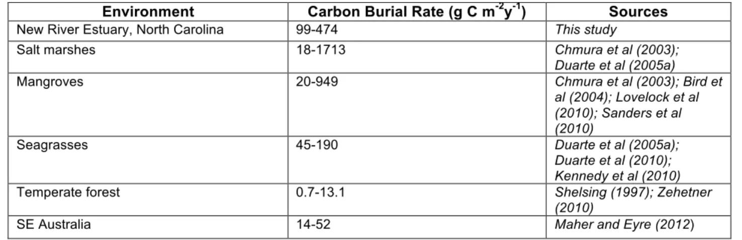
Mean carbon burial rates in the NRE were calculated by multiplying the mean accretion rate by the Carbon density. NRE-1 and NRE-2 had the lowest average carbon burial rates of 100.82 g C m-2 yr-1 and 99.46 g C m-2 yr-1. NRE-3 had higher average carbon burial rates, 135.34 g C m-2 yr-1. Most notably, NRE-4 had average carbon burial rates of 474.09 g C m-2 yr-1,four times the carbon burial rates at the upper estuary sites and double the rate at NRE-6. NRE-6, the most seaward core had average carbon burial rates of 280.40 g C m-2 yr-1, still more than double the rates at NRE-1, NRE-2, and NRE-3, but only about half the rates at NRE-4. These values are listed in Table 2.

NRE-1, 2, and 3 have similar trends of carbon burial rates over the last 100-150 years, a steady increase until the peak in 1999, followed by a decrease, but rates returning to pre-peak values about five years prior to coring date. NRE-4 has significantly higher carbon burial rates (note the different scale on the y-axis of Figure 5.) and multiple peaks of high burial. The highest peak of carbon burial in NRE-4 is dated about 9 years in the past, which agrees with the peaks in MAR and SAR (see 6.4 and 6.5). Carbon burial rates at NRE-6 have more distinct peaks at about 54, 29, and 14 years in the past but otherwise a steady increase over time with a sharp decline approximately seven years prior to core collection in 2013 (about 2006) which corresponds to the years of peaks in the MAR and SAR.

Figure 5 shows Carbon density in black, accretion rate in red and carbon burial rate in blue for NRE-2, NRE-4, and NRE-6 and years before present on the x-axis. Carbon density was calculated by multiplying dry bulk density by the percent carbon in each sample. These plots show carbon density remaining fairly constant while accretion rate and carbon burial vary significantly in conjunction with each other indicating that accretion rate, not carbon density, is the primary driver of carbon burial in the New River Estuary.

Core ID

Mean Carbon burial rate (g C m-2 yr-1)

NRE-1 100.82

NRE-2 99.46

NRE-3 135.34

NRE-4 474.09

NRE-6 280.40

0 100 200 300 400 500 600 700 800 900 1000 0.0 0.5 1.0 1.5 2.0 2.5 3.0 3.5 4.0 4.5 5.0 0 20 40 60 80 100 Ca rb on B u ri al R at e[ g/ (m 2*y) ] C d en si ty * 7 5 Accr eti

on Rate (cm/

y) Years BP

NRE-4

0 100 200 300 400 500 600 700 800 900 1000 0.0 0.5 1.0 1.5 2.0 2.5 3.0 3.5 4.0 4.5 5.0 0 20 40 60 80 100 Ca rb on B u ri al R at e[ g/ (m 2*y) ] C d en si ty * 7 5 Accr eti

on Rate (cm/

y) Years BP

NRE-6

0 50 100 150 200 250 300 350 400 0.0 0.2 0.4 0.6 0.8 1.0 1.2 1.4 1.6 1.8 2.0 0 20 40 60 80 100 Ca rb on B u ri al R at e [g/ (m 2*y) ] C d en si ty * 3 0 Accr eti

on Rate (cm/

y)

Years BP

7.DISCUSSION

Nichols 1993 described a stepwise process of sedimentation during and following a hurricane event in an estuary- temporary accumulation in the upper estuary, scouring and seaward transport, and accumulation in the lower estuary. The data presented in this study supports this hypothesis with a high-resolution sedimentary record of a preserved storm event in the New River Estuary obtained from the analysis of 210Pb geochronology.

7.1 Conclusion of Models

All of these geochronology models are valuable when interpreting 210Pb data. To get the best results, data should be applied to all models and assumptions should be evaluated and validated via secondary chronostratigraphic or non-chronostratigraphic markers. The CRS model proved most relevant given the nonmonotonous XS 210Pb profiles and changing sediment and mass accumulation rates. A natural stratigraphic marker aided in the validation of the dates given by the CRS model. The peaks in sedimentation rates within each core corresponded exactly with the dates of hurricanes Dennis and Floyd.

7.2 Total Inventories

NRE-1, NRE-2 and NRE-3 have 210Pb inventory values that are slightly lower or slightly higher than the mean values cited by Graustein and Turekian (1986) and Benninger and Wells (1993) for sites in North Carolina where inventories were supported solely by atmospheric flux (26.52 dpm cm-2,). NRE-4, and NRE-6 have inventory values that are much higher than the mean inventory supported by

NRE (Wallace and French creek), which, during heavy rain events might deposit more sediment and associated 210Pb than other areas of the estuary. The 210Pb activity of particulate matter being discharged by these tributary streams is undocumented but are likely low. The lower surface 210Pb activity and higher surface SAR and MAR values are consistent with an input of sediment from tributary streams during the months prior to the collection of the core.

7.3 Mass and Sediment Accumulation Rates

The mass accumulation rates and sediment accumulation rates in the New River Estuary vary greatly throughout the estuary, but they all retain the relic peak of the 1999 storm event. The SAR 1999 peak appears to occur at a slightly more recent date in the geochronologies of the cores down estuary. The resolution in the upper few centimeters of the cores is slightly higher than one year. Down-core, the resolution degrades. The peak at NRE-1 was dated at 1999 while the peak at NRE-2 was dated at 2000, NRE-3 dated at 2001, NRE-4 dated at 2006, and NRE-6 dated back at 2000. NRE-1, 2, 3, and 6, within error, have peaks in direct correlation with the date that tropical storm Dennis and hurricane Floyd made landfall in Onslow county. The SAR peaks in NRE-4 appear to have occurred at a later date than any of the other cores. There is no clear explanation for this at present, but it is hypothesized that this occurred because of erosion. This part of the estuary serves as a depositional hot spot as indicated by

sedimentation rates, mass accumulation rates, and inventory. Additional sediment supply to NRE-4 is hypothesized to come from nearby tributaries and/or from redistribution of sediment from elsewhere in the estuary as a result of deposition and erosion cycles. The dynamic nature of this area sets it apart. It is possible that a recent erosional event, followed by sediment input from adjacent streams would have resulted in a net loss of the sediment top, making the SAR peak appear to be more recent. It is also possible that the surface of this core was altered during the core retrieval process.Since it is only the date of the SAR peak that is affected (the MAR peak is consistent with the other cores at ~1999-2000) then perhaps another explanation lies in the bulk density profile.

most core, affected the most by high energy events. NRE-4 and NRE-6 retain more peaks in the sedimentary record because they are higher energy than the upper estuary, but are still relatively large lagoonal features that act as settling basins. High SAR provides higher resolution geochronologies- enough to show multiple peaks. These basins have much higher preservation of the sediment deposited there because of the high SAR and MAR rates. The faster the sediment is buried, the more likely it is to be retained in the sediment record.

7.4 Carbon Burial Rates

Environment Carbon Burial Rate (g C m-2y-1) Sources

New River Estuary, North Carolina 99-474 This study

Salt marshes 18-1713 Chmura et al (2003);

Duarte et al (2005a)

Mangroves 20-949 Chmura et al (2003); Bird et

al (2004); Lovelock et al (2010); Sanders et al (2010)

Seagrasses 45-190 Duarte et al (2005a);

Duarte et al (2010); Kennedy et al (2010)

Temperate forest 0.7-13.1 Shelsing (1997); Zehetner

(2010)

SE Australia 14-52 Maher and Eyre (2012)

8.CONCLUSION

APPENDIX 1. PLOTS FROM NRE-1 AND NRE-3

NRE-1.

0

0.5

1

1.5

2

2.5

3

3.5

4

0 2 4 6 8 10 12 14

mi

(g

cm-2

)

NRE-1 XS 210_Pb

210_Pb

1865 1875 1885 1895 1905 1915 1925 1935 1945 1955 1965 1975 1985 1995 2005 2015

0.00 0.50 1.00 1.50

SAR (cm yr-1₎

1865 1875 1885 1895 1905 1915 1925 1935 1945 1955 1965 1975 1985 1995 2005 2015

0.0 0.1 0.2 0.3

MAR (g cm-2 _yr-1₎

0 50 100 150 200 250 300 350 400 0.0 0.2 0.4 0.6 0.8 1.0 1.2 1.4 1.6 1.8 2.0 0 20 40 60 80 100 Ca rb on B u ri al R at e [g/ (m 2*y) ] C d en si ty * 3 0 Accr eti

on Rate (cm/

y)

NRE-3

0.0

0.5

1.0

1.5

2.0

2.5

3.0

3.5

4.0

0 2 4 6 8 10 12

mi

(g cm

-2

)

NRE-3 XS 210_Pb

210_Pb

1925 1935 1945 1955 1965 1975 1985 1995 2005 2015

0.00 0.50 1.00 1.50

1925 1935 1945 1955 1965 1975 1985 1995 2005 2015

0.00 0.10 0.20 0.30 0.40

MAR (g cm-2 _yr-1₎

0 50 100 150 200 250 300 350 400 0.0 0.2 0.4 0.6 0.8 1.0 1.2 1.4 1.6 1.8 2.0 0 20 40 60 80 100 Ca rb on B u ri al R at e [g/ (m 2*y) ] C d en si ty * 3 0 Accr eti

on Rate (cm/

y)

APPENDIX 2. COMPARISON TO OTHER MODELS

Core

ID Inventory (dpm cm-2

) Initial

210_Pb XS

Concentration

(dpm g-1

)

Mean CFCS SAR

(cm yr-1

)

Mean CRS SAR

(cm yr-1

)

Mean CIC SAR

(cm yr-1

)

Mean CFCS MAR

(g cm-2

yr-1

)

Mean CRS MAR

(g cm-2

yr-1

)

Mean CIC MAR

(g cm-2

yr-1

REFERENCES

Appleby, P. G. (2002). Chronostratigraphic Techniques in Recent Sediments. Tracking Environmental Change Using Lake Sediments, 171-203. doi:10.1007/0-306-47669-x_9

Appleby, P. G., & Oldfield, F. (1983). The assessment of 210Pb data from sites with varying sediment accumulation rates. Paleolimnology, 29-35. doi:10.1007/978-94-009-7290-2_5

Benninger, L. K., & Wells, J. T. (1993). Sources of sediment to the Neuse River estuary, North Carolina. Marine Chemistry, 43(1-4), 137-156. doi:10.1016/0304-4203(93)90221-9

Blanchard, R. (1966). Rapid determination of lead-210 and polonium-210 in environmental samples by deposition on nickel. Analytical Chemistry. 38(2). 189-192.

Bricker, S. B., C. G. Clement,D. E. Pirtalla,S. P. Orlando , and D. R. G. Farrow.1999. National Estuarine Eutrophication Assessment: Effects of Nutrient Enrichment in the Nation's Estuaries. National Oceanic and Atmospheric Administration, National Ocean Service, Special Projects Office and the National Centers for Coastal Ocean Science. Silver Spring, Maryland.

Burkholder, J. M., & Glaskow, H. B. (2001). History of Toxic Pfiesteria in North Carolina Estuaries from 1991 to the Present. BioScience, 51(10), 827.

doi:10.1641/0006-3568(2001)051[0827:hotpin]2.0.co;2

Canuel, E.A., & Hardison, A.K. (2016). Sources, Ages, and Alteration of Organic Matter in Estuaries. Annual Review of Marine Science. 8(1), 409-434

Card, J. W., & Bell, K. (1985). The relationship of soil 210Po and 210Pb geochemical dispersion patterns to uranium mineralization. Journal of Geochemical Exploration,23(2), 101-115.

doi:10.1016/0375-6742(85)90021-4

Dalrymple, R. W., Zaitlin, B. A., & Boyd, R. (1992). Estuarine facies models; conceptual basis and stratigraphic implications. Journal of Sedimentary Research, 62(6), 1130-1146.

doi:10.1306/d4267a69-2b26-11d7-8648000102c1865d

Dame, R., Alber, M., Allen, D., Mallin, M., Montague, C., Lewitus, A., … Kjerfve, B. (2000). Estuaries of the South Atlantic Coast of North America: Their Geographical Signatures.Estuaries, 23(6), 793. doi:10.2307/1352999

Elliott, E. A., McKee, B. A., & Rodriguez, A. B. (2015). The utility of estuarine settling basins for constructing multi-decadal, high-resolution records of sedimentation. Estuarine, Coastal and Shelf Science, 164, 105-114. doi:10.1016/j.ecss.2015.06.002

Flynn, W. (1968). The determination of low levels of polonium-210 in environmental materials.Analytica Chimica Acta, 43, 221-227. doi:10.1016/s0003-2670(00)89210-7

Graustein, W. C., & Turekian, K. K. (1986). 210 Pb and 137 Cs in air and soils measure the rate and vertical profile of aerosol scavenging. J. Geophys. Res, 91(D13), 14355.

doi:10.1029/jd091id13p14355

Hedges, J. I., & Keil, R. G. (1995). Sedimentary organic matter preservation: an assessment and speculative synthesis. Marine Chemistry, 49(2-3), 137-139. doi:10.1016/0304-4203(95)00013-h Herrmann, M., Najjar, R. G., Kemp, W. M., Alexander, R. B., Boyer, E. W., Cai, W., … Smith, R. A.

Hurricane Floyd. (n.d.). Retrieved from http://www.weather.gov/mhx/Sep161999EventReview Jia, G., Torri, G., Petruzzi, M., (2004). Distrubution coefficients of polonium between %5 TOPO in

toluene and aqueous hydrochloric and nitric acids. Applie Radiation and Isotopes. 61(2-3), 279-282.

Mallin, M. A., McIver, M. R., Wells, H. A., Parsons, D. C., & Johnson, V. L. (2005). Reversal of eutrophication following sewage treatment upgrades in the New River Estuary, North Carolina. Estuaries, 28(5), 750-760. doi:10.1007/bf02732912

Martin, A., & Blanchard, R. L. (1969). The thermal volatilisation of caesium-137, polonium-210 and lead-210 from in vivo labelled samples. The Analyst, 94(119), 441-446. doi:10.1039/an9699400441

Martin, P., Hancock, G.J., 2004. Routine analysis of naturally occurring radionuclides in environmental samples by alpha-particle spectro- metry. Supervising Scientist Report 180, AGPS, Canberra Mattheus, C. R., & Rodriguez, A. B. (2010). Controls on late Quaternary incised-valley dimension along

passive margins evaluated using empirical data. Sedimentology, 58(5), 1113-1137. doi:10.1111/j.1365-3091.2010.01197.x

Matthews, K. M., Kim, C., & Martin, P. (2007). Determination of 210Po in environmental materials: A review of analytical methodology. Applied Radiation and Isotopes, 65(3), 267-279.

doi:10.1016/j.apradiso.2006.09.005

Mcleod, E., Chmura, G. L., Bouillon, S., Salm, R., Björk, M., Duarte, C. M., … Silliman, B. R. (2011). A blueprint for blue carbon: toward an improved understanding of the role of vegetated coastal habitats in sequestering CO2. Frontiers in Ecology and the Environment, 9(10), 552-560. doi:10.1890/110004

Nichols, M. M. (1993). Response of coastal plain estuaries to episodic events in the Chesapeake Bay Region. Nearshore and Estuarine Cohesive Sediment Transport, 1-20. doi:10.1029/ce042p0001 NOAA. 1996. NOAA's Estuarine Eutrophication Survey, Volume 1: South Atlantic Region. NOAA, Office

of Ocean Resources Conservation Assessment, Silver Spring, Maryland

NOAA. (n.d.). Background- History of the Intracoastal Waterway Route “Red Line” Retrieved from http://www.nauticalcharts.noaa.gov/IntracoastalWaterwayRoute/Historical%20background%20Int racoastal%20Waterway%20Route%20magenta%20line.pdf

NOAA. (n.d.). Hurricanes. Retrieved from https://coast.noaa.gov/hurricanes/ NOAA. (n.d.). Tropical Storm Dennis - Early September 1999. Retrieved from

http://www.wpc.ncep.noaa.gov/tropical/rain/dennis1999.html

NOAA's National Ocean Service Education: Estuaries. (2011, July 18). Retrieved from http://oceanservice.noaa.gov/education/tutorial_estuaries/welcome.html

NuDat 2.6. (2012). Retrieved from www.nndc.bnl.gov/nudat2/reCenter.jsp?z=82&n=128

Sanchez-Cabeza, J. (1998). Simultaneous determination of radium and uranium activities in natural water samples using liquid scintillation counting. The Analyst, 123(2), 399-403.

Sanchez-Cabeza, J., & Ruiz-Fernández, A. (2012). 210Pb sediment radiochronology: An integrated formulation and classification of dating models. Geochimica et Cosmochimica Acta, 82, 183-200. doi:10.1016/j.gca.2010.12.024

Western Lake Catchment Systems. (n.d.). Retrieved from http://gec.cr.usgs.gov/archive/lacs/lead.htm Zhu, J., & Olsen, C. R. (2013). Sedimentation and Organic Carbon Burial in the Yangtze River and