Robustness of the Shrinkage Estimator for
the Relative Potency in the Combination of
Multivariate Bioassays
Ding-Geng (Din) Chen
School of Social Work
University of North Carolina-Chapel Hill, NC 27599, USA
Department of Statistics, University of Pretoria, Pretoria, South Africa
Email: [email protected]
Abstract
This paper investigates the robustness of the shrinkage Bayesian estimator for the
relative potency parameter in the combinations of multivariate bioassays proposed
in Chen et al.(1999), which incorporated prior information on the model
parame-ters based on Jeffreys’ rules. This investigation is carried out for the families of
t-distribution and Cauchy-distribution based on the characteristics of bioassay
the-ory since the t-distribution approaches the normal distribution which is the most
commonly used distribution in the applications of bioassay as the degrees of freedom
increases and the t-distribution approaches the Cauchy-distribution as the degrees
of freedom approaches 1 which is also an important distribution in bioassay. A real
data is used to illustrate the application of this investigation. This analysis further
supports the application of the shrinkage Bayesian estimator to the theory of bioassay
along with the empirical Bayesian estimator.
1
Introduction
Estimation of relative potency in biological assay (i.e. bioassay) is very important in
phar-maceutical and toxicological sciences. A variety of methods for estimating relative potency
can be found in the literature and the references in Finney (1978) and Govindarajulu
(2001). Most of these methods can be formulated in terms of a general linear model for
data following a normal distribution, or in a generalized linear model for other types of
data. In the situation of multi-response experiments, multivariate statistics can be used as
in Laska et al. (1985), Srivastava (1986) and Chen et al. (1999).
The combination of bioassays arises when the same or similar experiment is performed
by multi-laboratories and multi-centers in the calibration of national/international
stan-dards for a particular substance (Rose and Gaines-Das, 1998). With the studies of
com-bination of bioassays, most results appear in Bennett (1962), Armitage (1970), Meisner et
al. (1986), William (1988), Chen et al. (1999), Xiong and Chen (2007), and Chen (2007).
Chen et al. (1999) proposed a novel empirical Bayesian estimator (EBE) and a
shrink-age Bayesian estimator (SBE) for the relative potency from the combination of several
multivariate bioassays by incorporating prior information on the model parameters based
on Jeffreys’ rules. The EBE can account for any extra-variability among the bioassays,
and if the extra-variability is zero, the EBE reduces to the maximum likelihood estimator
for combinations of bioassays. The SBE estimator turned out to be a weighted average of
the prior information and the estimator from each bioassay with the weights depending on
the prior variance, which is not uncommon in Bayesian framework. The key advantage of
this shrinkage Bayesian estimator is that it can be written in closed form and therefore no
iterative process is involved to yield the estimate.
However any prudent Bayesian analysis should include an investigation of the robustness
of the posterior distribution to the specifications of commonly used prior distributions.
theory into a bioassay framework by using the Jeffreys’ theory for the model parameters.
This technique takes the advantage that some information is known about the log relative
potency parameter µ, while little information is known about the other parameters from the model specification of the combination of multivariate bioassays. Therefore, the robust
investigation for the shrinkage Bayesian estimator is given to different specifications of the
prior distribution for the parameter of µ.
In this paper, the families of t- and Cauchy-distributions will be investigated for the robustness analysis since practically t-distribution is considerably important, especially for the heavy-tail distribution. As the degrees of freedom increases, the t-distribution ap-proaches the normal distribution, which is the most commonly situation in the applications
of bioassay as illustrated in Finney (1978) and Chen et al. (1999). On the other hand, as
the degrees of freedom approaches 1, thet-distribution approaches the Cauchy distribution, which is also an important distribution in bioassay since the log relative potency estimator
is a ratio of two normal variables, which is distributed as a Cauchy distribution.
This paper is organized as follows. Section 2 introduces the bioassay model and
shrink-age Bayesian estimator based on Jeffreys’ prior from Chen et al. (1999) and the
investiga-tion of two families of t-distribution and Cauchy-distribution is given in Section 3. A real data analysis is illustrated in Section 4 with further discussions given in Section 5.
2
Combinations of Bioassays and Shrinkage Estimator
2.1
Model Specification
The experimental model for ith (i= 1,· · ·, k) multivariate bioassay in the combinations of
k multivariate bioassays to estimate the relative potency of the test (t) preparation to the standard (s) preparation is usually of the following form:
yti = αti+βtixti+ti (2.1)
where ysi,yti ∈ Rp, p ≥ 1, are multivariate responses in the dose-response relationship, αsi, αti, βsi, βti ∈ Rp are the multivariate parameters, and xsi, xti are the scalar inputs as function of dose levels.
This model can then be casted in a multivariate regression framework
Yi =ΨiXi +i, (2.2)
whereYi = (ys1, . . . ,ysnsi,yt1, . . . ,ytnti) is thep×nimatrix of responses withni =nsi+nti,
where nsi, nti are the number of observations in the ith bioassay for the standard and test preparations, respectively; and Ψi = (αi,δi,βi) is the p×3 matrix of parameters. For all i = 1, . . . , k, 0is are assumed i.i.d. ∼ Np(0,V), where V is p×p positive definite symmetric matrix.
Different assumptions on the model parameters can produce different bioassay models.
There are two commonly-known bioassays with one as parallel-line bioassay and another
as slope-ratio bioassay. In the parallel-line bioassays where the two slopes in equation (2.1)
on both test preparation (i.e. βti) and standard preparation (i.e. βsi) are equal (denoted
by βi) where βi = βsi = βti, (see for example, Carter and Hubert (1985) for the test of
the parallelism), but with different intercepts so thatαi =αsi;δij =αtij−αij =µijβij, for all bioassays i= 1, . . . , k, and all responses j = 1, . . . , p, whereµij are scalar parameters, which are the log relative potencies of the ith bioassay and jth response variable. The slope-ratio bioassay has slightly different parameterizations where the slopes are different
but the intercepts are the same, such that αi = αsi = αti, δi = δti = µijβsi where µij are the relative potencies in ith bioassay and jth response variable. We will illustrate parallel-line bioassay in this paper and the similar discussions can be made for slope-ratio
bioassay.
normal random vectors Np(0,V); and Xi is the 3× ni design matrix defined as Xi =
1 · · · 1 1 · · · 1 0 · · · 0 1 · · · 1
xs1 · · · xsnsi xt1 · · · xtnti
, where x’s are log dose levels. Then the multivariate
regression technique can be used to obtain the estimators
ˆ
Ψi = YiX0i(XiX0i)
−1
(2.3)
Si = m−i 1Yi h
I−X0i(XiX0i)
−1 X
i i
Y0i (2.4)
as independent estimators ofΨi andV, wheremi =ni−3 andX0 is the transpose of matrix
X. Since our interest is in the relative potency parameterµij, the second and third columns of ˆΨi will be the relevant ones, while the parameters in the first column, ˆαi, are the nuisance
parameters. Therefore, we will restrict our attention to ˆ δi ˆ βi
∼ N2p δi βi
,V⊗Ai , where Ai is the lower 2×2 portion of (XiX0i)−1.
To block diagonalize the matrix V⊗Ai in order to make ˆδi and ˆβi independent, let’s define Ti =
t11i t12i 0 t22i
, such that TiAiT0i = I. Then, t11i =
a122/2i
(a11ia22i−a122 i)1/2, t12i =
−a12ia −1/2 22i
(a11ia22i−a212i)1/2 andt22i =a
−1/2
22i . Letui =t11iδˆi+t12iβˆiandvi =t22iβˆi, then the distribution of ui and vi is
ui
vi ∼N2p
t11iδi+t12iβi
t22iβi
,V ⊗I2
. (2.5)
In addition,Siin equation (2.4) is distributed asSi ∼m−i 1Wp(V, mi) = Wp(V/mi, mi), which is the Wishart distribution, a multivariate generalization of the Chi-square
distribu-tion, with the pdf given by Ci|V|−
mi
2 |Si|mi
−p−1
2 etr(−mi
2 V
−1S
i), where etr is the notation for exponent of the trace, |V| is the determinant of matrixV and Ci is a constant of inte-gration chosen so that the total probability is 1 (Srivastava and Carter, 1983). The pooled
estimator for V is thenS= (Pk
2.2
Shrinkage Bayesian Estimator for the Log Relative Potency
The shrinkage estimator was derived in Chen et al. (1999) based on Jeffreys’ prior (Hoadley,
1970) of π(µ,βi,V)∝ h(µ)
|V|(p+1)/2 with h(µ)∼N(µ0, τ
2), for someµ
0 and τ2 >0.
It was shown that µ|Xi, Yi,βi,V ∼N(µp, τp2),where
µp =
τ2Pk
i=1t11iβ0iV
−1(t
11iδiˆ +t12iβˆi−t12iβi) +µ0
τ2Pk
i=1t211iβ
0
iV−1βi+ 1
τp = k X i=1
t211iβ0iV−1βi+ 1
τ2
!− 1 2
.
Then the shrinkage Bayesian estimator(SBE) for the log relative potency, µ, can be obtained using the estimates in equations (2.3) and (2.4) for βi and V as follows:
µSBE =
τ2Pk
i=1t211iβˆi
0
S−i 1δiˆ +µ0
τ2Pk
i=1t211iβˆi
0
S−i 1βˆi+ 1 (2.6)
τSBE = k X i=1
t211iβˆi0S−i 1βˆi+ 1
τ2
!− 1 2
. (2.7)
Therefore the credible region with (1-α)100% coefficient for µcan be expressed as µSBE±
zα/2τSBE where zα/2 is the usual percentile point such that 1 - Φ(zα/2) = α/2, and where
Φ(·) is the cumulative distribution function for a standard normal random variable. The corresponding noninformative shrinkage Bayesian estimator can be obtained by
letting τ approaches infinite as follows:
ˆˆ
µ = Pk
i=1t211iβˆi
0
S−i 1δˆi Pk
i=1t211iβˆi
0
S−i 1βˆi
(2.8) ˆ ˆ τ = k X i=1
t211iβˆi0S−i 1βˆi !−
1 2
. (2.9)
Similar (1-α)100% credible region forµcan be expressed as ˆµˆ±zα/2ˆτˆ.
The advantage for this shrinkage Bayesian estimator and its interval estimator described
above is that they can be calculated explicitly from the model parameter estimates which
3
Robust Analysis for the Shrinkage Bayesian
Esti-mator
Since, in most practical situations, some information can be known about the relative
potency, µ and relatively little information is known about βi and V, then by Jeffreys’ rules, a suitable prior distribution would beπ(µ,βi,V)∝ |V|h(p(+µ)1)/2, whereh(µ) is a proper
prior distribution for µ. Then the posterior distribution of µ, conditional on Xi, Yi, βi and V can be shown from equation (2.5) as follows:
µ|Xi,Yi,βi,V∝π(µ,βi,V) L(µ,βi,V)
∝ h(µ)exp
(
−1
2 k X i=1
(t11iδˆi+t12iβˆi−t11iµβi−t12iβi)
0
V−1(t11iˆδi+t12iβˆi−t11iµβi−t12iβi) )
.
(3.1)
The posterior function (3.1) incorporates all the information from the data by the
likelihood function and prior information from h(µ). Parallel to the maximum likelihood theory, an estimate of the log relative potency can be obtained by maximizing the posterior
likelihood function, i.e. estimating the log relative potency parameter by the mode of the
posterior likelihood function. Another alternative is to estimate the log relative potency
parameter by the median or mean of the posterior likelihood function. This estimator is usually referred as the posterior Bayesian estimator (Mood et al. 1973). However if
the prior distribution is normal, these two alternatives produce same estimators, since
the posterior distribution is also normally distributed. Actually, if h(µ) is the normal distribution N(µ0, τ2) and after simple manipulations, the same results in Section 2.2 can
be derived.
For the posterior Bayesian estimator, numerical integration is involved to obtain this
estimator. Therefore, to be concise for this robustness analysis and also parallel to the
con-ventional likelihood estimation, the mode of the posterior likelihood function (3.1) is used
This estimator is then referred to as the shrinkage estimator (SBE). The same analysis can
be carried out for posterior Bayesian estimator.
3.1
Robustness of Shrinkage Estimator under
t
-Prior Density
Ifµis distributed as a t-distribution withn(n >0) degrees of freedom, location parameter
µ0 and scale parameter τ, then the density function is:
h(µ) = Γ( n+1
2 )
Γ(n2) 1 √ nπ 1 τ 1 h
1 + 1n(µ−µ0 τ )2
in+12
, −∞< µ <∞, (3.2)
whereE(µ) =µ0 andV ar(µ) = nn−2 τ2 (−∞< µ0 <∞,τ > 0). It can be shown that the
larger n value or the smallerτ value, the more peaked for the distribution and as n→ ∞,
V ar(µ) → τ2, which is the smallest value for V ar(µ). Theoretically, for sufficient larger value of n, the t-distribution is back to normal distribution.
The shrinkage estimator can be obtained by taking the derivative of (3.1) with respect
to µand letting it to be zero. The following equation is obtained:
2aµ3+ (−b−4aµ0)µ2+ (−1−n+ 2bµ0+ 2anτ2+ 2aµ20)µ−bnτ 2+nµ
0+µ0−bµ20 = 0. (3.3)
It can be shown that there is only one real root for this equation which is
µ(n;µ0, τ) =
1 6
J(n;µ0, τ)
2
3 −6ag2+g2
1 −g1J(n;µ0, τ)
1 3
aJ(n;µ0, τ)
1 3
, (3.4)
where:
J(n;µ0, τ) = 9ag1g2−54a2g3−g13+ 3
√
3a(8ag23−g12g22−36ag1g2g3+ 108a2g32+ 4g 3 1g3)
1 2
g1 = −b−4aµ0
g2 = −1−n+ 2bµ0+ 2anτ2+ 2aµ20
g3 = −bnτ2+nµ0+µ0−bµ20
a = −1
2 k X i=1
t211iβi0V−1βi
b = −
k X i=1
t11iβi
0
Since the parametersβi andV are unknown, the true value of this shrinkage estimator
is unknown. However, independent estimates of βi and V are available from (2.3) and
(2.4). Thus, an empirical shrinkage estimator can be formed by replacing the estimators
from (2.3) and (2.4) into (3.4) as follows:
ˆ
µ(n;µ0, τ) =
1 6
ˆ
J(n;µ0, τ)
2
3 −6ˆaˆg2+ ˆg2
1 −gˆ1Jˆ(n;µ0, τ)
1 3 ˆ
aJˆ(n;µ0, τ)
1 3
, (3.5)
It can be easily proven from (3.5) that
ˆ
µ(n;µ0, τ)→
ˆbτ2−µ 0
2ˆaτ2−1 =
ˆb−µ0/τ2
2ˆa−1/τ2 as n → ∞. (3.6)
which is the shrinkage Bayesian estimator (µSBE) obtained in equation (2.6). Therefore ˆ
µ(n;µ0, τ) → ˆb
2ˆa = ˆµˆ (i.e. the estimator in equation (2.8)) as n → ∞ and τ → ∞ which is insensitive to the different specifications of the prior density and is just a function of
the data. That is to say, in this situation, this empirical shrinkage estimator from t-family is very robust to various specifications of the prior parameters. In fact, as n → ∞, the
t-distribution is back to normal distribution and also, as τ → ∞, the empirical shrink-age estimator ˆµ(n;µ0, τ) approaches the noninformative shrinkage Bayesian estimator, ˆµˆ,
proposed in Chen et al. (1999), which is
ˆ ˆ
µ= Pk
i=1t211iβˆi
0
S−i 1δˆi Pk
i=1t211iβˆi
0
S−i 1βˆi
. (3.7)
This estimator ˆµˆ represents a noninformative or uniform prior and can be rewritten as ˆˆ
µ = Pk i=1 t2 11i ˆ βi 0
S−1
i
ˆ
βi
Pk i=1t
2 11i
ˆ
βi 0
S−1
i
ˆ
βi
ˆ
µi, which is the weighted average of estimators of log relative potency fromith bioassay, ˆµi, with the weights depending only on the maximum likelihood estimates of the model parameters. Therefore, in the situation of no prior information, this
estimator (ˆµˆ) is recommended.
The above outcomes strongly suggests that in the t-distribution and normal distri-bution, the shrinkage Bayesian estimator proposed in Chen et al. (1999) is robust for
Bayesian estimator. However, the noninformative shrinkage Bayesian estimator ˆµˆ is prior-independent and possesses the advantages that ˆµˆ is the weighted average of estimators of log relative potency from each bioassay with the weights depending only on the maximum
likelihood estimates of the model parameters. It can be used to estimate the log relative
potency in the bioassay theory.
3.2
Robustness of Shrinkage Estimator under Cauchy
Distribu-tion
Not only is the Cauchy prior distribution the extreme situation in the Section 3.1 when
n = 1, but also it is special in the theory of bioassay. The well-known fact in bioassay theory is that the estimated log relative potency is the ratio of two normal variables. But
the ratio of two normal variables is distributed as a Cauchy distribution. From this point
of view, the Cauchy distribution is relatively more important. In this section, the Cauchy
distribution is considered as the prior for the robustness analysis.
If µ is distributed by a Cauchy distribution, then the density function is h(µ) =
1
πτ{1+(µ−µ0
τ )2}
, where τ > 0 is the scale parameter and µ0 (−∞ < µ0 < ∞) is the
lo-cation parameter. The same procedures as in Section 3.1 yields the shrinkage estimator:
µ(µ0, τ) = −
1 6
−J
2 3
µ0,τ −12a+ 12a
2τ2−4a2µ2
0+ 4abµ0−b2−4aµ0J
1 3
µ0,τ −bJ 1 3 µ0,τ
aJ
1 3 µ0,τ
, (3.8) where:
Jµ0,τ = −[36a
2µ
0−18ab+ 72a3τ2µ0−36a2bτ2+ 8a3µ30−12a 2bµ2
0+ 6ab 2µ
0−b3
−6√3a(−16a+ 4abµ0 + 80a3τ2µ20+ 20aτ
2b2+ 32a4τ4µ2 0+ 8a
2b2τ4
+16a4τ2µ40+τ2b4+ 48a2τ2−4a2µ20−b2−48a3τ4+ 16a4τ6 −80a2bτ2µ0
−32a3τ2bµ30+ 24a2τ2µ20b2−8aτ2b3µ0 −32a3τ4bµ0)
1 2]
a = −1
2 k X i=1
t211iβi0V−1βi
b = −
k X i=1
t11iβi
0
Then the empirical shrinkage estimator can be obtained by replacing the estimators
from (2.3) and (2.4). This results in:
ˆ
µ(µ0, τ) = −
1 6
−Jˆ
2 3
µ0,τ −12ˆa+ 12ˆa2τ2−4ˆa2µ20+ 4ˆaˆbµ0−ˆb2−4ˆaµ0Jˆ
1 3
µ0,τ −ˆbJˆ 1 3 µ0,τ ˆ
aJˆ
1 3 µ0,τ
, (3.9)
Similarly, it can be proven that
ˆ
µ(µ0, τ)→µˆˆ as τ → ∞. (3.10)
In this case the empirical shrinkage estimator again approaches the noninformative
shrink-age Bayesian estimator proposed in Chen et al. (1999).
3.3
The Ideal Shrinkage Estimator
The results from both Sections 3.1 and 3.2 imply that as µ0 →µˆˆ, the empirical shrinkage
estimator ˆµ(n;µ0, τ) in (3.5) and ˆµ(µ0, τ) in (3.9) will both be robust irrespective of the
prior variance τ2. That is to say, if the data contain sufficient information to make the
prior distribution concentrate on the prior means, or the prior distribution is chosen to
match the data “perfectly”, then the empirical shrinkage estimator is very robust to
differ-ent specifications of prior. Otherwise, if the prior disagrees sharply with the information
contained in the data, the empirical shrinkage estimator is less robust.
Therefore, to estimate the log relative potency in combination of bioassays, the plausible
procedure is to use the estimators from (2.3) and (2.4) to estimate a prior mean and
prior standard deviation on any k − 1 of k bioassays. Next utilize them as the prior information to form the final shrinkage estimator for the last bioassay, which is robust
and has all the properties previously described. Hence, it is named as the ideal shrinkage
estimator. This ideal shrinkage estimator is superior to the general shrinkage estimator
and the noninformative shrinkage estimator because the prior distribution is formulated
4
Data Analysis
Data was originally from Finney (1978). In illustrating the combination of multivariate
bioassays, Meisner, Kushner and Laska (1986) artificially broke up the data into two
mul-tivariate bioassays with the first bioassay using the twelve bivariate responses from lines 1
and 3 and the second bioassay using the twelve bivariate responses from lines 2 and 4. The
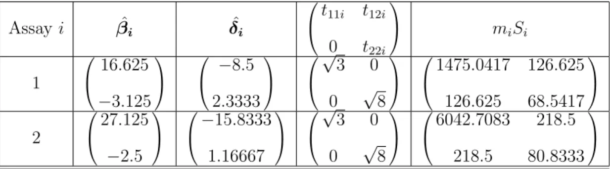
summary statistics are given in Table 1 for the two assays.
Table 1: Summary Statistics of the Two Assays
Assayi βˆi δˆi
t11i t12i 0 t22i
miSi
1
16.625
−3.125
−8.5 2.3333
√ 3 0
0 √8
1475.0417 126.625 126.625 68.5417
2
27.125
−2.5
−15.8333 1.16667
√ 3 0
0 √8
6042.7083 218.5 218.5 80.8333
As seen in Chen et al (1999), the test for equality of covariance can not be rejected
since the test statistic is 4.107, which is less than χ2
3,0.05=7.815. Consequently we can use
the pooled variance-covariance as follows:
S=
417.653 19.174 9.174 8.299
.
Based on these values, the noninformative shrinkage estimate for the overall log relative
potency ˆµˆin equation (2.8) can be calculated to be -0.590 with 95% CI as (-1.039, -0.141), suggesting the test preparation is significantly less potent than the standard preparation
in this combination of bioassays.
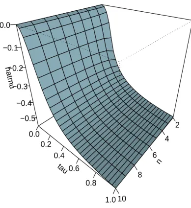
To graphically illustrate the robustness analysis in Section 3, Figure 1 displays this
empirical shrinkage estimator ˆµ(n; 0, τ) in equation (3.5) versus n and τ for fixed µ0 = 0
based on this data. It can be seen from Figure 1 that even though the shrinkage estimator
ˆ
sufficiently large enough, the empirical shrinkage estimator ˆµ(n;µ0, τ) quickly approaches
the noninformative empirical Bayesian estimator ˆµˆ in equation (2.8) and appears to be robust irrespective of the specifications of n, µ0 and τ int-distribution family.
n
2
4
6
8
10
tau
0.0 0.2
0.4
0.6
0.8
1.0
hatm
u
−0.5 −0.4 −0.3 −0.2 −0.1 0.0
Figure 1: µˆ(n; 0, τ ) as the function of n and τ with the prior of t-distribution.
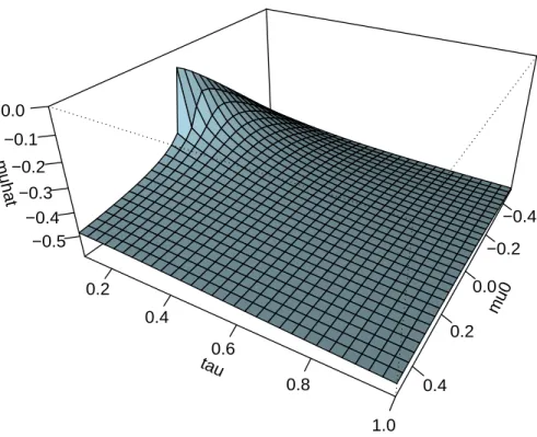
Similar conclusion can be made for the empirical shrinkage estimator ˆµ(µ0, τ) in
equa-tion (3.9) versus µ0 and τ as shown in Figure 2. It can be seen from Figure 2 that if
τ is sufficiently large, ˆµ(µ0, τ) quickly approaches the noninformative empirical Bayesian
estimator ˆµˆ in equation (2.8) and appears to be robust irrespective of the value at µ0. If
mu0 −0.4
−0.2
0.0
0.2
0.4
tau
0.2
0.4
0.6
0.8
1.0
m uhat
−0.5 −0.4 −0.3 −0.2 −0.1 0.0
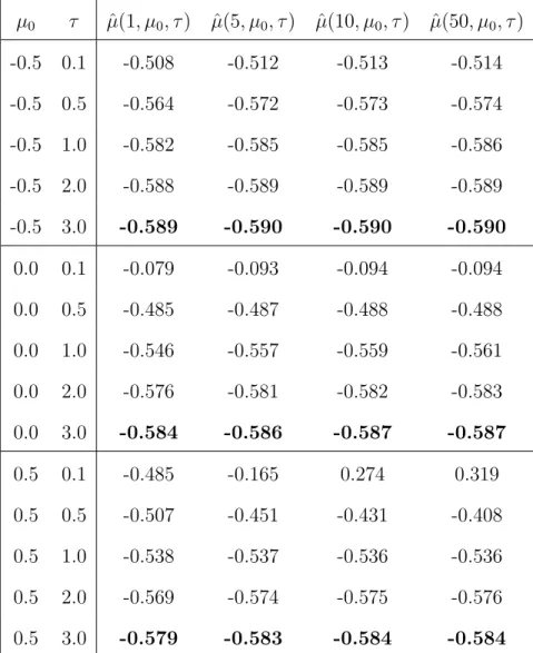
To numerically illustrate the robustness, Table 2 gives the values of the empirical
shrink-age estimator ˆµ(n, µ0, τ) in equation (3.5) for several specifications of n, µ0 and τ. In the
table, four values of n = 1,5,10,50 are illustrated which are column-headed by ˆµ(1, µ0, τ),
ˆ
µ(5, µ0, τ), ˆµ(10, µ0, τ) and ˆµ(50, µ0, τ). The first column ˆµ(1, µ0, τ) is in fact ˆµ(µ0, τ) in
equation (3.9) since whenever n= 1, the t-distribution becomes the special case of Cauchy distribution and therefore ˆµ(n, µ0, τ) in equation (3.5) would be ˆµ(µ0, τ) in equation (3.9).
The last column ˆµ(50, µ0, τ) illustrates the empirical shrinkage estimator with large degrees
of freedom from t-distribution which would be very similar to the normal prior. Therefore this last column would mimic the shrinkage Bayesian estimator µSBE in equation (2.6) as proposed in Chen et al (1999). The middle two columns illustrate the t-distribution between Cauchy and normal distributions.
In Table 2, three values ofµ0 are chosen whereµ0 =−0.5 is close to the noninformative
empirical estimator ˆµˆ = −0.590 and other two values of 0 and 0.5 are chosen farther away from ˆµˆ. Five values of τ are chosen from 0.1 (small), 0.5, 1, 2 to 3 (large). It can be clearly seen from Table 2 that all ˆµ(1, µ0, τ), ˆµ(5, µ0, τ), ˆµ(10, µ0, τ) and ˆµ(50, µ0, τ) rapidly
approach the ˆµˆ = −0.590 irrespective of the different specifications of µ0 and τ. This is
especially true with µ0 = −0.5 which again indicates that when an appropriate prior is
selected, the three shrinkage estimators of µSBE in equation (2.6), ˆµ(n, µ0, τ) in equation
(3.5) and ˆµ(µ0, τ) in equation (3.9) could all approximate the noninformative shrinkage
Bayesian estimator ˆµˆ in equation (2.8).
This leads to the ideal shrinkage estimator proposed in Section 3.3 to use any k−1 of the k bioassays as the prior information to compute a prior mean ˆµ0 using equation (2.8)
and prior standard deviation ˆτ0 using equation (2.9) and then utilize these values to form
the final shrinkage estimator using equations (2.6) and (2.7) with the kth bioassay. This can be easily implemented for this data. We take the first bioassay to compute a prior
mean ˆµ0 using equation (2.8) and prior standard deviation ˆτ0 using equation (2.9) which
Table 2: Numerical illustration of the empirical Bayesian estimator ˆµ(n, µ0, τ) for different
specifications of n = 1, 5, 10, 50, µ0 = −0.5, 0, 0.5 and τ = 0.1, 0.5, 1.0, 2.0, 3.0. The
bolded values indicate ˆµ(n, µ0, τ) approaches the noninformative shrinkage estimator ˆµˆ=
−0.590.
µ0 τ µˆ(1, µ0, τ) µˆ(5, µ0, τ) µˆ(10, µ0, τ) µˆ(50, µ0, τ)
-0.5 0.1 -0.508 -0.512 -0.513 -0.514
-0.5 0.5 -0.564 -0.572 -0.573 -0.574
-0.5 1.0 -0.582 -0.585 -0.585 -0.586
-0.5 2.0 -0.588 -0.589 -0.589 -0.589
-0.5 3.0 -0.589 -0.590 -0.590 -0.590
0.0 0.1 -0.079 -0.093 -0.094 -0.094
0.0 0.5 -0.485 -0.487 -0.488 -0.488
0.0 1.0 -0.546 -0.557 -0.559 -0.561
0.0 2.0 -0.576 -0.581 -0.582 -0.583
0.0 3.0 -0.584 -0.586 -0.587 -0.587
0.5 0.1 -0.485 -0.165 0.274 0.319
0.5 0.5 -0.507 -0.451 -0.431 -0.408
0.5 1.0 -0.538 -0.537 -0.536 -0.536
0.5 2.0 -0.569 -0.574 -0.575 -0.576
calculate a final estimate using equations (2.6) and (2.7) from the second bioassay. In this
situation, these two equations are actually reduced to:
µIdeal = ˆ
τ2 0t2112βˆ2
0
S−1δˆ 2+ ˆµ0
ˆ
τ2 0t2112βˆ2
0
S−1βˆ + 1 (4.11)
τIdeal = t2112βˆ2
0
S−1βˆ2+ 1 ˆ
τ2 0
!−12
. (4.12)
And they are estimated asµIdeal =−0.590 and τIdeal = 0.229 with associated 95% CI as (-1.039,-0.141). Similarly if we take the second bioassay to compute the prior mean ˆµ0 and
prior standard deviation ˆτ0, we can get ˆµ0 = −0.543 and ˆτ0 = 0.302. Using these values
in the normal prior to calculate the final estimate using equations (4.11) and (4.12) on the
first bioassay, we can obtain µIdeal =−0.590 andτIdeal = 0.229 with associated 95% CI as (-1.039,-0.141) which yields the exact numeric values.
All the calculations in this section are done in R (a free software available from
http://www.r-project.org) and the R program can be requested from the author.
5
Discussion
In this paper the investigation of the robustness of the shrinkage Bayesian estimator was
conducted for two commonly-known families of t-distribution and Cauchy-distribution. It was shown that the shrinkage estimator would change for different specifications of
differ-ent prior distributions. But if the prior variance is large enough or the prior information
matches the “data”, the shrinkage estimator is robust and approaches the noninformative
shrinkage Bayesian estimator which is insensitive to different specifications of prior
distri-bution and is only data-dependent. A real data analysis demonstrated these conclusions.
As seen from the data analysis, the three shrinkage estimators from the normal
If the prior information is indeed available, the shrinkage Bayesian estimator proposed
in Chen et al. (1999) can be readily applied to the prior information directly and hence
a Bayesian estimator can be calculated using the procedures in this paper. Otherwise,
the ideal shrinkage estimator proposed in Section 3.3 could be adopted for the estimation
of the relative potency for combination of bioassays. This ideal shrinkage estimator was
demonstrated to be valid and applicable which also produced the same results as the
noninformative shrinkage Bayesian estimator from the real data analysis.
In fact, the procedure in this paper is very general and can be used for any specification
of the prior density. Not only can it be used for robust analysis, it can also be used to
propose different Bayesian estimators under different prior specifications. As a summary, it
can be concluded that the Bayesian approach is a recommended in the theory of bioassay.
Furthermore, this newly-developed Bayesian procedure is applicable for the combination
of univariate bioassays (Xiong and Chen 2007), combination of multivariate bioassays,
parabolic bioassays (Chen 2010), as well as combination of parabolic bioassays. It has
been shown that it is superior to some conventional methods. The robust investigation in
this paper makes a good conclusion for its properties and provides a strong recommendation
for its use. Hence, the Bayesian method is a natural way to improve the theory of bioassay.
Acknowledgements
I am grateful for the useful suggestions and comments from the two reviewers, Professor
Balakrishnan and Dr. Nicole Trabold which greatly improved the draft manuscript.
References
[1] Armitage, P. (1970). The combination of assay results. Biometrika, 57: 665-666.
[2] Bennett, B.M. (1962). On combining estimates of relative potency in bioassay.Journal
[3] Carter, E. M. and Hubert, J. J. (1985). Analysis of parallel-line assays with
Multivari-ate responses. Biometrics, 41: 703-710.
[4] Chen, D. G., Carter, E. M., Hubert J. J. and Kim, P. T.(1999). Empirical Bayesian
estimation for combinations of multivariate bioassays. Biometrics, 55(4): 1035-1043.
[5] Chen, D. G. (2007). Bootstrapping Estimation for Relative Potency in the
Combina-tions of Bioassays. Computational Statistics and Data Analysis, 51: 4597-4604.
[6] Chen, D. G. (2010). Estimate the relative potency in parabolic bioassay. Journal of
Advances and Applications in Statistical Sciences. 2(1): 1-18.
[7] Finney, D. J. (1978).Statistical Method in Biological Assay. Third Edition. C. Griffin,
London.
[8] Govindarajulu, Z. (2001).Statistical Techniques in bioassay. Karger PubliSBErs
(USA).
[9] Hoadley, B.(1970). A Bayesian look at inverse linear regression. Journal of the
Amer-ican Statistical Association, 65: 357-369.
[10] Laska, E. M., Kushner, H. B. and Meisber, M(1985). Multivariate bioassay.Biometrics,
41: 547-554.
[11] Meisner, M., Kushner, H. B. and Laska, E. M.(1986). Combining multivariate
bioas-says. Biometrics, 42: 421-427.
[12] Mood, A. M., Graybill, F.A. and Boes, D.C.(1974). Introduction to the Theory of
Statistics. McGraw-Hill, Inc.
[13] Rose, M. P. and Gaines-Das, R. E.(1998). Characterisation, calibration and
compari-son by international collaborative study of international standards for the calibration
[14] Srivastava, M. S.(1986). Multivariate bioassay, combination of bioassays and Fieller’s
theorem. Biometrics, 42: 131-141.
[15] Srivastava, M.S. and Carter, E.M.(1983). An Introduction to Applied Multivariate
Statistics. North-Holland, New York.
[16] Williams, D.A.(1988). An exact confidence region for a relative potency estimated
from a multivariate bioassays. Biometrics, 44: 861-867.
[17] Xiong, J. and Chen, D. G. (2007). A Shrinkage Estimator for Combination of