PRIORITIZING CONTENT OF INTEREST IN MULTIMEDIA DATA COMPRESSION
Chong Shao
A dissertation submitted to the faculty of the University of North Carolina at Chapel Hill in partial fulfillment of the requirements for the degree of Doctor of Philosophy in the
Department of Computer Science.
Chapel Hill 2018
Approved by: Shahriar Nirjon Russell M. Taylor II David Brady
©2018 Chong Shao
ABSTRACT
CHONG SHAO: Prioritizing Content of Interest in Multimedia Data Compression (Under the direction of Shahriar Nirjon and Russell M. Taylor II)
Image and video compression techniques make data transmission and storage in digital multi-media systems more efficient and feasible for the system’s limited storage and bandwidth. Many generic image and video compression techniques such as JPEG and H.264/AVC have been stan-dardized and are now widely adopted. Despite their great success, we observe that these standard compression techniques are not the best solution for data compression in special types of multi-media systems such as microscopy videos and low-power wireless broadcast systems. In these application-specific systems where the content of interest in the multimedia data is known and well-defined, we should re-think the design of a data compression pipeline. We hypothesize that by identifying and prioritizing multimedia data’s content of interest, new compression methods can be invented that are far more effective than standard techniques. In this dissertation, a set of new data compression methods based on the idea of prioritizing the content of interest has been proposed for three different kinds of multimedia systems.
ACKNOWLEDGEMENTS
TABLE OF CONTENTS
TABLE OF CONTENTS . . . vii
LIST OF TABLES . . . xiii
LIST OF FIGURES . . . xv
LIST OF ABBREVIATIONS . . . xx
1 Introduction . . . 1
1.1 Research Questions . . . 3
1.1.1 How to Better Compress Digital Videos with Specific Usages? . . . 3
1.1.2 How to Better Compress Digital Images that Transmitted Through a Band-width Constrained System? . . . 3
1.1.3 How to Compress Multiple Types of Application Data in a Bandwidth Constrained System? . . . 4
1.1.4 How to Apply Generative Models in Extreme Compression? . . . 4
1.2 A Brief Outline of the Proposed Methods . . . 4
1.2.1 Content-Prioritizing Correlation-Based Microscopy Video Compression . . 4
1.2.2 Extreme Image Compression that Enables Image Beacons . . . 5
1.2.3 Feature Selection and Key Point Extraction that Enables Indoor Augmented Reality Data Transmission over BLE Broadcasting . . . 5
1.2.4 Generative Image Compression . . . 5
1.3 Thesis and Contributions . . . 6
1.4 Organization of the Rest of the Dissertation . . . 8
2 Background . . . 9
2.2 Lossless Compression . . . 10
2.2.1 Variable Length Coding . . . 10
2.2.2 Dictionary Transform . . . 11
2.2.3 Contextual Transform . . . 12
2.2.4 Context Adaptive Variable Length Coding and Context Adaptive Variable Binary Arithmetic Coding . . . 13
2.3 Prediction/Residual Framework . . . 14
2.4 Multimedia Compression . . . 15
2.4.1 Discrete Cosine Transform . . . 16
2.4.2 Discrete Wavelet Transform . . . 17
2.5 Previous Work on Domain-Specific Video Multimedia Data Compression . . . 17
2.5.1 Region-Prioritizing Video Compression methods . . . 18
2.5.2 Video Compression Methods That are Built on Existing Standards . . . 19
2.6 Miscellaneous Topics in Modern Multimedia Compression . . . 20
2.6.1 Point Spread Function in Image and Video Acquisition Process . . . 20
2.6.2 Bandwidth Limited Transmission Channel: Bluetooth Low Energy Broad-casting Mode . . . 21
2.6.3 Multimedia Data Quality Evaluation Using Statistical Tests . . . 22
3 Video Compression to Preserve Analysis-Critical Information . . . 24
3.1 Related Work . . . 25
3.2 Overview . . . 27
3.2.1 Analysis-Preserving Compression . . . 27
3.2.2 Analysis-Aware Compression . . . 29
3.2.3 Statistical Tests . . . 30
3.3 Methods . . . 31
3.3.1 Segmentation Stage . . . 33
3.3.3 Post-Processing Stage . . . 37
3.3.4 Analysis-Aware Video Quality Measurement . . . 38
3.4 Results . . . 40
3.4.1 Analysis-Preserving Compression Results . . . 40
3.4.2 Analysis-Aware Compression Results . . . 45
3.5 Summary . . . 55
4 Image Compression to Generate Energy Efficient Broadcast Image Data . . . 58
4.1 Related Work . . . 63
4.2 BLE System Characterization . . . 65
4.3 Image Beacon and Use Cases . . . 66
4.3.1 Long-term Surveillance Systems . . . 67
4.3.2 Navigation Systems . . . 67
4.3.3 Internet of Everything Minus the Internet . . . 67
4.3.4 New Applications . . . 67
4.4 Challenges in Building an Image Beacon . . . 68
4.4.1 Limited BLE Bandwidth . . . 68
4.4.2 The Case for Lossless Image Broadcast . . . 69
4.4.3 The Case for Compressed Image Broadcast . . . 69
4.5 Algorithm Design . . . 71
4.5.1 Patch-Based Binary Image Compression Algorithm . . . 71
4.5.2 Overview of the Color Image Beacon System . . . 75
4.5.3 Multiview Capture and Depth Estimation . . . 78
4.5.4 Color Image Encoding . . . 83
4.6 Empirical Evaluation . . . 88
4.6.1 Image Beacon Implementation Details . . . 88
4.6.3 Color Image Beacon System Evaluation . . . 94
4.7 Real Deployment . . . 101
4.7.1 Write-Read-Recognize . . . 101
4.7.2 Navigation in the Building . . . 104
4.8 Summary . . . 107
5 Extraction and Compression of Augmented Reality Content for Low Power Augmented Reality System . . . 108
5.1 Related Work . . . 111
5.2 Overview of MARBLE . . . 112
5.2.1 Two Phases of MARBLE . . . 114
5.2.2 Internal Modules and Basic Workflow . . . 114
5.2.3 Advantage of MARBLE . . . 115
5.3 Application Content Generation . . . 116
5.3.1 Visual Features . . . 117
5.3.2 Selecting Unique and Useful Features . . . 118
5.3.3 Storing Camera Properties . . . 119
5.3.4 Generating AR Content . . . 119
5.4 Real-Time AR Content Rendering . . . 120
5.4.1 BLE-based Location and Viewing Angle Estimation . . . 121
5.4.2 Camera-based Location and Viewing Angle Estimation . . . 121
5.4.3 Fusion of Multiple Sensor Inputs . . . 122
5.4.4 Rendering Objects . . . 123
5.5 Implementation Notes . . . 123
5.6 Evaluation . . . 124
5.6.1 Microbenchmarks . . . 124
5.6.2 Algorithm Evaluation . . . 127
6 Generative Compression as an Alternative Approach to Extreme Compression . . . 133
6.1 Introduction . . . 133
6.2 Related Work . . . 135
6.3 System Architecture . . . 136
6.3.1 Offline Training . . . 137
6.3.2 Online Capture, Broadcast, and Render . . . 138
6.4 Algorithm . . . 139
6.4.1 Background on Variational Autoencoder (VAE) . . . 139
6.4.2 Background on Generative Adversarial Networks (GAN) . . . 139
6.4.3 VAE-GAN in Deep Beacon . . . 139
6.4.4 Compressed VAE-GAN Embedding . . . 140
6.5 Embedding Size Reduction Algorithm . . . 140
6.6 Data Packet Format . . . 141
6.7 Evaluation . . . 142
6.7.1 Experimental Setup . . . 142
6.7.2 The Choice of Embedding Size . . . 144
6.7.3 Comparision with JPEG Encoding . . . 145
6.7.4 Performance on Different Image Types . . . 146
6.7.5 Impact of Number of Beacons . . . 146
6.7.6 User Study . . . 147
6.7.7 Comparison with Other Image Beacon Systems . . . 149
6.8 Summary . . . 149
7 Conclusion and Discussion . . . 151
7.1 Summary of Contributions . . . 151
7.1.1 Microscopy Video Compression . . . 151
7.1.3 MARBLE: Augmented Reality Application Data Compression for
Blue-tooth Low Energy Devices . . . 153
7.2 Discussion and Future Work . . . 154
7.2.1 Microscopy Video Compression . . . 154
7.2.2 Image Compression for BLE Beacons . . . 154
7.2.3 MARBLE: Augmented Reality Application Data Compression for Blue-tooth Low Energy Devices . . . 156
7.3 Remaining Technical Issues . . . 156
7.3.1 MARBLE: Generic Gesture Capture and Rendering . . . 156
7.3.2 Smart Packet Rotation Strategy in Bluetooth Low Energy Broadcasting . . 157
7.3.3 No-Calibration Deployment for MARBLE . . . 157
LIST OF TABLES
2.1 Comparison between common compression standards. . . 15
2.2 Comparison between common two-sample statistical tests. . . 23
3.1 Compression ratio for five real-world videos. The analysis-preserving method outper-formed standard H.264 compression by large factors in three out of five test cases. In both cases, the resulting compressed video is in H.264 format so can be easily fed into analysis pipelines. . . 40 3.2 Comparison of multiple compression methods on four of the videos shown in the main
text. The left and right numbers match those in TABLE 1. Bzip2 and lossless JPEG2000 compression on the original file sequence were usually worse and never much better than lossless H.264. Lossless JPEG2000 and Bzip2 on the filtered image set were always worse than lossless H.264. . . 41
3.3 Maximum tracking error when using lossy compression techniques and using my method in four cases (in units of the experiment noise floor, which is 101th of a pixel). In one video, a bead track was lost, indicated here as infinite error. When they are forced to achieve the same compression ratios, perceptually-tuned compression techniques have a large maximum impact on analysis results. . . 42
3.4 Mean and standard deviations of tracking error when using lossy compression tech-niques and using my method in four cases (in units of experiment noise floor, which is 1/10th of a pixel). . . 42
3.5 Compression ratio using the sliding window method and using lossless H.264 alone for the Fastbeads video. With longer windows, the beads moved across essentially every pixel in the image, so the method produced almost no improvement over lossless H.264 alone. With very short windows noise suppression was slightly reduced, causing an increase in file size. The optimal window size for this video was 20 frames, resulting in an approximately 2 improvement in file size. As expected, smaller dilation results in better compression (less fore-ground). . . 44 3.6 Achieved compression ratios for applying analysis-aware methods and lossless
com-pression method on synthetic data and real data and maintain KS test p-score larger than 0.95 in the resulting video. For synthetic data, an improvement of around a factor of 2 was achieved above the earlier lossless method. For real data, which had more noise, the improvement was around a factor of 350. . . 54
5.3 CPU and memory usage of Smartphone . . . 127
LIST OF FIGURES
1.1 Comparison between common generic image/video compression (a) and
prior-itizing content of interest compression (b). . . 2
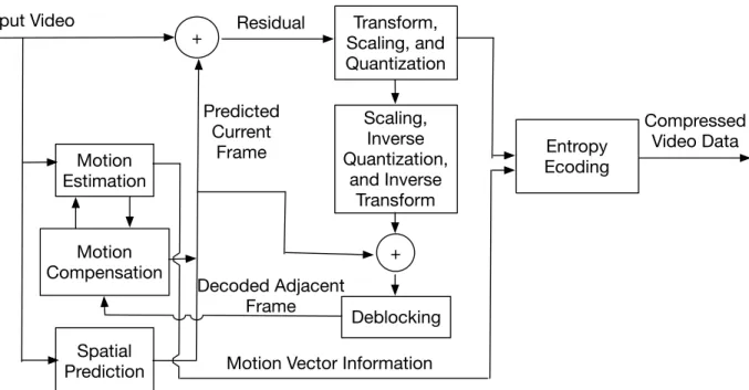
2.1 H.264 encoder and decoder as an example of prediction/residual framework. . . 15
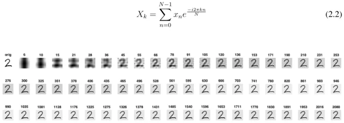
2.2 Sample hand-written digit image (4096 bytes) and the DCT-compressed version of the image with the compressed size in bytes. . . 16
2.3 A 2D PSF convolved with a sample image, generates a blurred image. . . 21
3.1 Analysis-preserving video compression process. . . 28
3.2 Analysis-aware video compression process. . . 30
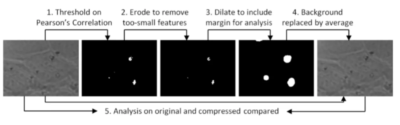
3.3 Mathematical morphology portions of the original algorithm: (a) a sub region of the first frame in the original video; (b) the correlation-based segmentation result without refinement; (c) the segmentation result after erosion refinement; (d) the segmentation result after erosion and dilation refinement. Some fore-ground regions in (d) are due to other beads that move into this region in later frames. . . 33
3.4 Plots of compressed file size comparing against original file size (in percentage) vs. correlation magnitude threshold on scores for four videos. Four subplots shows the result for four test videos respectively. Four plots share the same vertical axis. The horizontal flat line in every subplot indicates the compression result on that video with H.264 lossless technique. The curves become dashed when the analysis results on compressed videos differs from the analysis result on the original, indicating the limit compression without impacting analysis results. . . 34
3.5 Example frame from each of the videos tested, each named as in the description and tables. . . 35
3.6 Left to right: a) the starting position of a bead in a video and its moving trajectory; b) the resulting binary foreground/background map; c) illustration of the macroblocks that covers the frame; d) the resulting binary macroblock foreground/background labeling map. . . 37
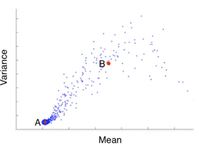
3.7 Mean vs. variation intensity plot with centers of the two-means cluster. . . 39
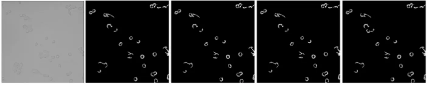
3.9 Left to right: first frame of the original video, edge detection results: original video, video with 3.5×compression, video with 4.6×compression, video with
6.8×compression. . . 45
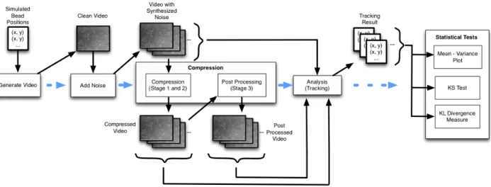
3.10 Flow chart of the experiment steps with synthetic data . . . 46
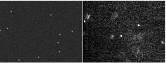
3.11 Sample video frames, left: synthetic video, right: real video . . . 47
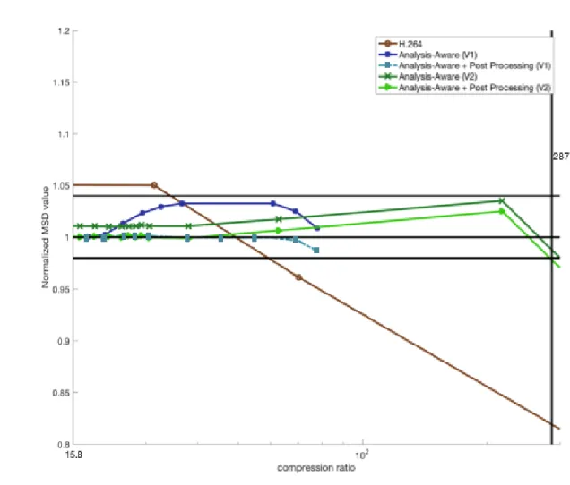
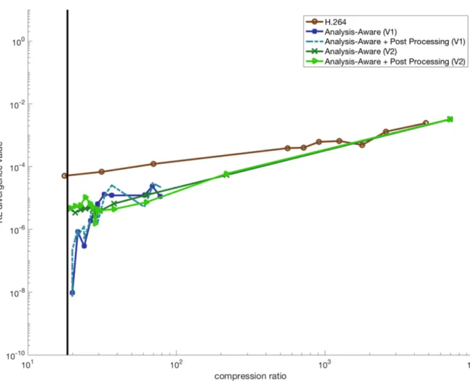
3.12 Scaled MSD values vs. compression ratio, for five groups of synthetic videos. . . 49
3.13 KS test p values vs. compression ratio. The horizontal line shows the KS test p score 0.95. The vertical line in every plot shows the compression ratio for the previous analysis-preserving method. . . 50
3.14 K-L divergence values vs. compression ratio, for five groups of synthetic videos. The vertical line in every plot shows the compression ratio for the previous analysis-preserving method. . . 52
3.15 Flow chart of the experiment steps with real data. . . 53
3.16 Scaled MSD values vs. compression ratio, for five groups of real videos. . . 54
3.17 KS test p values vs. compression ratio. The two horizontal lines showing the KS test p score 0.95 and 0.99, respectively. The vertical line in every plot shows the compression ratio for the previous analysis-preserving method. . . 55
3.18 K-L divergence values vs. compression ratio, for five groups of real videos. The vertical line in every plot shows the compression ratio for the previous analysis-preserving method. . . 56
4.1 An image beacon system. . . 59
4.2 The lifetime depends on packet transmission rate and signal strength. . . 69
4.3 A 64×64 resolution image compressed in high/low quality settings using JPEG/JPEG2000: (a) JPEG high quality, 1963 bytes (b) JPEG2000 high quality, 2026 bytes (c) JPEG lowest possible quality, 738 bytes (d) JPEG2000 lowest possible quality, 391 bytes. . . 70
4.4 Two types of 64×64 resolution image compressed in PNG (a) from natural scene, 12112 bytes (b) JPEG2000 high quality, 1012 bytes. PNG is good for handling images with large uniform color regions. . . 70
4.5 Beacon image processing pipeline. . . 71
4.7 (a) original image; (b) result from patches generated from single spiral image; (c) result image from patches generated from single spiral image after mor-phology refinement; (d) result image from patches generated from multiple spiral images and k-means; (e) result from patches generated from multiple
spiral images and k-means after morphology refinement. . . 74
4.8 Image processing stages. . . 77
4.9 Multiple views of a scene are used to estimate the depth map. Combined with standard image segmentation, this can identify the pixels of an image that may be of more interest than the rest, e.g. a foreground object. . . 78
4.10 Image compression details. . . 83
4.11 64×64 resolution building image compressed in high/low quality settings using my customized DCT/Wavelet/Triangle encoding: (a) Original image, (b) DCT 342 bytes, (c) Wavelet high 360 bytes, (d) DCT 1114 bytes, (e) Wavelet 1098 bytes, and (f) triangularization 366 bytes. For a similar compressed image size, DCT preserves less details than Wavelet method. But for low quality settings (about 350 bytes), Wavelet-encoded images have strange color block defects. Triangularization failed to preserves the information in the original image. . . 84
4.12 Original image and the triangularization-compressed image. . . 86
4.13 The process of Triangularization-based encoding. . . 87
4.14 Triangle texture averaging process. . . 88
4.15 Test images used in the empirical evaluation. . . 90
4.16 Image quality versus image size for different encoding methods. . . 91
4.17 Image quality versus beacon battery life for different images being approxi-mated. . . 91
4.18 Image quality versus device lifetime for various number of beacons. . . 92
4.19 Image quality versus lifetime for different patch generation methods. . . 93
4.20 Image quality versus device lifetime for various patch set sizes. Note that the patch set with sizek=16 is not simply a subset of the patch set of sizek=32. They are individualk-means clustering results with differentks. . . 94
4.21 Image quality versus device lifetime for various grid sizes per patch. . . 95
4.22 Test images used in the empirical evaluation. . . 96
4.23 Performance of IMU-guided view capture. . . 97
4.25 Image quality versus image size for different encoding methods. . . 98
4.26 Image quality versus beacon battery life for different image types. . . 100
4.27 Image quality versus device lifetime for various number of beacons. . . 100
4.28 Subjective and SSIM scores for each image. . . 102
4.29 Test images compressed in three quality levels. . . 103
4.30 Photos of the object used in the experiment. . . 104
4.31 Responses from user study. The dashed line shows 33 percent chance of randomly choosing. . . 104
4.32 Map of second and third floors showing the navigation path. . . 105
4.33 Images stored at the six locations. . . 106
4.34 Subjective scores for each image. . . 106
5.1 The two phases of MARBLE indoor augmented reality system: capture (once) and render (many times). . . 109
5.2 System in Action. (a): in capture phase, a person’s gesture and movement is captured. (b): in render phase, the virtual object avatar is rendered in the empty environment. (c): screenshot of the viewer’s screen in render phase. . . 113
5.3 A block diagram illustrating the work flow of MARBLE. . . 113
5.4 The process of feature filtering: hundreds of ORB features are extracted from a reference camera image in (a) and feature entropyθis computed. The resultant values are weighted by the 2D Gaussian function of (b). Four highest scored features are shown in a zoomed in region in (c). They are successfully matched with features extracted from a different image of the same scene even though some of the objects have been moved, as shown in (d). . . 117
5.5 The capture unit. . . 123
5.6 Run-time Analysis . . . 125
5.7 Energy Consumption of every stage of MARBLE. The data for the capture phase is colored in blue. The data for broadcasting phase is colored in green. The data for viewing phase is colored in orange. The power data next to the stage labels are the working power of each stage. The number next to the bar charts are the energy consumption for rendering a frame of the virtual object. . . 126
5.9 (a): the configuration of measurement points in the lab. (b): heat map showing
the number of cameras being considered in visual feature matching. . . 129
5.10 Heat Map of the errors in cm on location estimation in 16 different measure-ment points. From left to right: BLE Beacon based estimation, Camera based estimation and Sensor Fusion using two signals. . . 130
5.11 Heat Map of the errors in angle on pose estimation in 16 different measurement points. From left to right: IMU based estimation, Camera based estimation and Sensor Fusion using two signals. . . 130
5.12 Human Gesture Sampling Frequency Impact at (a) Low Speed (b) High Speed. . . 131
6.1 The proposed Deep Beacon system. . . 133
6.2 The data flow of Deep Beacon system. . . 137
6.3 VAE-GAN model structure. . . 137
6.4 The Deep Beacon data packet format. . . 141
6.5 Samples of training and test image dataset. First 4 rows from top row to bottom: hand-written digits, birds, traffic signs, and flowers. The last row contains sampled images compressed by Deep Beacon system. . . 143
6.6 Bar chart showing the average MS-SSIM of four types of image data with different embedding sizes. . . 144
6.7 MS-SSIM vs. Imgae size for 100 hand-written digit images (upper plot) and 100 traffic sign images (lower plot). Images are compressed using JPEG (red dots) and the encoder module in Deep Beacon system (blue dots). . . 145
6.8 Average MS-SSIM score vs. expected system lifetime plot. Four curves represent four types of testing data. Each curve represents one type of test image data. . . 146
6.9 Average MS-SSIM score vs. expected system lifetime plot. Three curves represent the experiment result with using one, two, and three beacons, respectively. . . 147
6.10 The traffic sign types used in user study. . . 148
6.11 The chance in percentage of a participant making a correct answer in recog-nizing hand-written digit images and traffic sign images compressed by Deep Beacon system. . . 148
LIST OF ABBREVIATIONS
AR Augmented Reality
ATT Low energy ATTribute protocol BLE Bluetooth Low Energy
CBA Customer Behavior Analysis
CISMM Computer Integrated Systems for Microscopy and Manipulation DCT Discrete Cosine Transform
DWT Discrete Wavelet Transform GAN Generative Adversarial Network GATT Generic ATTribute profile
GFSK Gaussian Frequency Shift Keying GPS Global Positioning System IMU Inertial Measurement Unit IoT Internet of Things
ISM band Industrial Scientific Medical band K-L KullbackLeibler
L2CAP Logical Link Control and Adaptation Protocol
LZ Lempel-Ziv
MARBLE Mobile Augmented Reality with Bluetooth Low Energy MSD Mean Square Displacement
ORB Oriented FAST and rotated BRIEF PSF Point Spread Function
QP Quantization Parameter ROI Region Of Interest
SURF Speeded Up Robust Feature SSIM Structure SIMilarity
CHAPTER 1 INTRODUCTION
Data compression is a process to take input data and to generate a compact representation of the input data with a shorter bit length. It is critical for many multimedia systems. With efficient data compression, transmission and storage of digital multimedia data become more affordable. During decades of development in the multimedia data compression field, a variety of popular multimedia compression methods including image and video compression methods have been standardized into CODEC specifications. Examples of the specifications are PNG, JPEG, and H.264. A multimedia compression specification typically includes a generic data compression component. They sometimes also include a smarter sampling strategy, a region of interest (ROI) data streaming or multimedia data modeling/parameterization and synthesis (Xu et al., 2014; Zhang and Bull, 2011; Balle et al., 2011).
New types of multimedia systems with specific purposes are constantly being built. Examples in recent years of the new systems include virtual reality headset (Oculus, 2015), augmented reality system (hol, 2017), high-throughput camera array system (Cribb et al., 2015), and low-power mobile data broadcasting “beacon” (ble, 2018). These new multimedia systems integrate advanced hardware such as a high-resolution display, low-power consumption chips and all types of sensors, along with new algorithms including high-accuracy object recognition and real-time scene understanding.
efficiently on these new systems. For example, a set of microscopy videos produced by an automatic microscope array system is only used by an analysis program in a cell-mechanics experiment pipeline. Most of the pixels in the video are never touched by the analysis program, but a generic video compression technique such as H.264 cannot accurately separate the useful information from noise in the microscopy videos. Another example is the designing of an “image beacon” system, where image data needs to be transmitted over Bluetooth low energy (BLE) broadcasting channel. The BLE broadcasting channel only has 30 bytes of payload size. However, the standard JPEG compression rarely compresses a 64×64 image smaller than 200 bytes.
During my Ph.D. work, I design compression techniques that are used for new types of multimedia systems. I will show that, prioritizing content of interest is one useful approach in creating new compression methods for these multimedia systems (Figure 1.1). This dissertation describes several examples of new multimedia systems and their challenges in data compression, followed by my solution to the problem.
1.1 Research Questions
In this section, I list the important questions I addressed in this dissertation.
1.1.1 How to Better Compress Digital Videos with Specific Usages?
We observe the increase of generated videos that have specific usages, especially videos that are analyzed by algorithms. Examples are surveillance videos and microscopy videos generated by analytical experiment pipelines. In some use cases such as a high-throughput screening (hig, 2017), there is a requirement to compress the video data to accommodate the limited storage. Standard video compression methods that assign equal importance to every pixel in the frame have difficulties in achieving small enough compressed video size. The question of how to identify the analysis-critical component in a microscopy video and how to generalize the analysis-critical component identification method are addressed in this dissertation.
1.1.2 How to Better Compress Digital Images that Transmitted Through a Bandwidth Con-strained System?
extreme compression method to compress a sufficiently large image (no less than 64×64 in size) into less than 200 bytes, so that the data can be carried by one a BLE 5.0 broadcasting packet?
1.1.3 How to Compress Multiple Types of Application Data in a Bandwidth Constrained System?
Some bandwidth-limited systems handle multiple types of data. It is an open problem to design a mechanism to handle data with different properties in such a system. I explored applying new compression methods in a bandwidth constrained system in compressing multiple types of data.
1.1.4 How to Apply Generative Models in Extreme Compression?
Recently, deep network models have shown strength in generating realistic fake image data. This opens the door to applying such a model in extreme compression. I also explored this direction.
1.2 A Brief Outline of the Proposed Methods
Here I list the methods I proposed in this dissertation, to address the questions in the last section.
1.2.1 Content-Prioritizing Correlation-Based Microscopy Video Compression
1.2.2 Extreme Image Compression that Enables Image Beacons
In building a self-contained image data storage and broadcast system using the BLE broad-casting channel, standard image compression techniques such as JPEG and PNG cannot generate sufficiently small compressed images. I design two new image compression methods that enable 64×64 dimension image storage and broadcast via BLE broadcasting channel. The first method is a dictionary-based patch matching binary image compression method. The second method is a foreground-preserving color image compression method that uses depth information in identifying the foreground in the input image.
1.2.3 Feature Selection and Key Point Extraction that Enables Indoor Augmented Reality Data Transmission over BLE Broadcasting
I demonstrate a data reduction approach for indoor augmented reality systems, which addresses question 1.1.3. Using BLE beacons as the storage and transmission component in an indoor AR system brings many benefits, such as long battery-powered lifetime, easy content data update, internet-free, and low cost. To overcome the challenges of small data bandwidth of Bluetooth Low Energy (BLE) protocol, I designed a 3D object data compression, along with a new entropy and location-based visual feature selection method. They enable indoor vision-based positioning and 3D content broadcasting via BLE broadcasting channel.
1.2.4 Generative Image Compression
1.3 Thesis and Contributions
Thesis: Some multimedia systems handle image or video data that has the notion of content of interest. Identifying and prioritizing image and video’s content of interest in these systems
lead to new image and video compression algorithms including analysis-preserving microscopy
video compression, analysis-aware microscopy video compression, patch-based binary image
compression, and adaptive color image encoding that enable smaller compressed data size that
prediction-residual based generic methods cannot achieve. With the smaller data size, the image
or video data compressed by prioritizing content of interest can also have the same quality as the
data produced by generic methods, measured with a generic image or video quality metric such as
Structural Similarity (SSIM).
In the following paragraphs, I highlight the contributions of this dissertation. Each contribution is labeled by the corresponding chapter number in this dissertation.
• I propose the first video compression technique in the literature that is based on correlation-based segmentation. The segmentation method identifies regions in the video that contain information. The compression method can achieve up to 20x better compression than H.264. I invent a correlation-based video frame segmentation technique based on the point spread function (PSF). I integrate the segmentation technique into the compression process. The PSF is involved in the imaging processes of a wide variety of optical systems. Therefore this segmentation method can be generalized to many video modalities (Chapter 3).
• I propose a new method to evaluate the quality of a microscopy video based on a statistical test. The method gives a video quality estimation based on the information loss of the analysis-critical part of the video. It takes the noise into consideration (Chapter 3).
• I develop and evaluate the first binary image beacon system. The evaluation compares the system performance under two instances of the binary image compression module trained with two different sets of data. The evaluation gives a deep insight of the system performance under different settings and proves its effectiveness in practice (Chapter 4).
• I propose a new color image compression method as a central component of a color image beacon system. This method takes the depth information of the object in the input image to generate an accurate segmentation for compressing the content of interest. It can generate less than 200 bytes of compressed image data. The method can be generalized into other use cases that require color image compression, and depth information of the image can be retrieved (Chapter 4).
• I develop and evaluate the first color image beacon system. The system supports storage and broadcast of color images of objects indoor and outdoors. My evaluation compares the system performance under different system settings and different types of input data. My user study with a real deployment of the system proves the system’s effectiveness in practice (Chapter 4).
• I develop and evaluate a new Internet-free beacon AR system that combines camera capture, IMU sensing input, and BLE signal strength in indoor positioning. The system provides a low-cost and extensible solution to indoor AR experience with common mobile devices (Chapter 5).
• I design and develop the first image beacon system that integrates variational autoencoder generative adversarial network (VAE-GAN). The system supports a wide range of binary and color images. It enables compression of a color 64×64 image into less than 20 bytes. I analyzed the system performance under different settings of the VAE-GAN model (Chapter 6).
1.4 Organization of the Rest of the Dissertation
CHAPTER 2 BACKGROUND
This chapter contains the background material related to my dissertation. Section 2.1 discusses Shannon’s Source Coding theorem, which builds the foundation of information theory. In Sec-tion 2.2, I highlight a set of lossless compression techniques. I give a brief introducSec-tion to each of them. Section 2.3 describes the prediction/residual framework that is used in many common multimedia compression systems. After that, in Section 2.4, I explain the important aspects of com-mon multimedia compression standards, including the two widely used signal transform methods. This is followed by a summary of existing domain-specific multimedia compression techniques in Section 2.5. I finish this chapter with Section 2.6. It includes several properties in multimedia systems that I used in building new compression methods and the background knowledge of new methodologies used in my compression algorithm design.
2.1 Shannon’s Source Coding Theorem
In 1948, Shannon formulated the source coding theorem (Shannon, 2001). The theorem gives a theoretical bound of the expected bit length of input codewords. The bound is a function of the entropy of the input symbols.
The mathematical version of the theorem is:
| 1
NHδ(X
N)−H|< (2.1)
HereHδ is the essential bit content, which is defined asHδ = log2|Sδ|, in which Sδ is the smallest subset that satisfiesP(x∈Sδ)≥1−δfor a givenδ.
A restatement of the theorem is that: having the input data asN independent and identically distributed (i.i.d.) random variables each with entropyH(X), it can be compressed into more than N H(X)bits with negligible risk of information loss, asN −→ ∞. On the other hand, if they are compressed into fewer thanN H(X)bits, it is virtually certain that information will be lost.
Shannon’s source coding theorem is tightly related to multiple lossless compression algorithms. However, it does not take the dependency between variables into consideration, which is widely used by many standard lossless compression algorithms such as contextual transform.
2.2 Lossless Compression
Lossless compression refers to the category of compression algorithms that generate compressed data that can be used to fully reconstruct the original data. In multimedia compression systems, lossless compression is usually used in an entropy coding stage, where the transformed multimedia data is losslessly encoded. In this section, I review three common lossless compression techniques: variable length coding (VLC), dictionary transform, and contextual transform. At the end of the section, I describe the two lossless compression methods that are customized for entropy encoding in video compression.
2.2.1 Variable Length Coding
The idea of variable length coding is to analyze the frequency of every codeword of the input data so that the symbols with shorter lengths are assigned to codewords that appear more frequently. Two most common examples are Huffman coding (Huffman, 1952) and arithmetic coding (Rissanen, 1976; McAnlis and Haecky, 2016). Both Huffman coding and arithmetic coding are used in the entropy coding stage of H.264 encoding process (Richardson, 2011).
The difference between Huffman coding and arithmetic coding is that Huffman coding uses symbols of integer length to represent each input codeword. Therefore, the symbol length may not exactly match the frequency of the corresponding codeword. Arithmetic coding addresses this problem by allowing floating number length of symbols. This is implemented by assigning intervals to each codeword at every encoding and decoding stage recursively. For example, we can assign symbolAto interval[0,0.7)and assign symbolBto interval[0.7,1]. Ais then represented by any floating number in interval[0,0.7). ABis represented by any floating number in interval [0.7∗0.7,1]. Compression is achieved from the shorter bit length for representing a floating number
comparing to the bit length of the original symbol sequence.
2.2.2 Dictionary Transform
A dictionary transform first builds a dictionary from the input data. It then uses the built dictionary to transform the data. The result is then sent to a statistical encoding routine such as VLC. Using dictionary transform as a pre-processing step before VLC makes the compression more effective. One example of dictionary transform is the Lempel-Ziv (LZ) transform (Ziv and Lempel, 1977).
To explain the LZ transform more precisely, I use an example: a current scanning buffer
TOBEORNOT, and the unscanned sequenceTOBET. So the entire input sequence of symbols in this example isTOBEORNOT|TOBET. The ‘|’ mark shows the current scanning position. The algorithm tries to match the longest sequence from the current scanning position in the current scanning buffer. The result isTOBE. This sequence is encoded as a pair of offset and length. In my example, it is(9,4). After this, the scanning buffer is shifted to the right by four steps. Now it is
ORNOTTOBE, and the current scanning position is also shifted to the right by four steps.
2.2.3 Contextual Transform
Contextual transform makes use of the contextual properties of the data. For example, in some types of data, adjacent codewords are more likely to have the same value. Hence, we can encode the sequence of repetitive codewords by a pair of a symbol and number of runs of that symbol. This transform is called run-length encoding. Run-length encoding is the most basic type of contextual transform. When the data tends to have successive increasing or decreasing values, starting from the second symbol, we can represent each symbol as the difference from the previous symbol. Then the result sequence of differences data will be more compactly represented by another pass of run-length encoding. This process is called delta-encoding.
I give an example of the process of the Burrows-Wheeler transform. I set the input sequence to be transformed asBANANA. The Burrows-Wheeler transform generates a list of sequences with length equal to the input sequence length by rotating the original sequence, and sorting by the first letter: ABANAN, ANABAN, ANANAB, BANANA, NABANA, NANABA. The transform output is the sequence of the last letter in the list:NNBAAA, and the index of the original sequence in the list: 3. This pair of items is sufficient for recovering the original input sequence. The Burrows-Wheeler
transform generates a sequence that is easier to compress because of the property that certain orders of a pair of tokens are more likely to appear in, as described in the last paragraph. Therefore, when the sequence of the first letter in the list is sorted, the corresponding sequence of the last letter is likely to have a repeating pattern.
2.2.4 Context Adaptive Variable Length Coding and Context Adaptive Variable Binary Arithmetic Coding
Context Adaptive Variable Length Coding (Karczewicz and Ridge, 2004) (CAVLC) and Context Adaptive Binary Arithmetic Coding (Marpe et al., 2003) (CABAC) are custom versions of VLCs for video compression. They are used in the entropy coding stage of H.264 and H.265 video compression standards. H.264 standard contains three types of profiles for different use cases. They are baseline profile, main profile, and high profile. In H.264, CAVLC is supported in all profiles. CABAC is only supported in main profile and high profile. CABAC can usually achieve a higher compression ratio. However, it requires more computation resource.
CABAC is similar to CAVLC because in both algorithms a probability model is selected among a set of candidates according to the current context. Differing from CAVLC, CABAC requires every input data to be binarized before compression. This is done by explicitly mapping every input symbol that is non-binary valued onto a sequence of binary decisions. It uses arithmetic coding rather than a look-up table.
2.3 Prediction/Residual Framework
We can extract a common pattern from the workflow from most multimedia compression systems. This pattern is named the Prediction/Residual Framework. The prediction/residual framework compresses data by making predictions on a subset of the data and use the prediction to produce a more compact representation of the data. A prediction can betemporalorspatial. A temporal prediction predicts a subset of the data based on other subsets of the data with a different timestamp. One example is that one frame in a video can be predicted from the previous frames. A spatial prediction predicts a sub-region in an image based other sub-regions in the same image.
Due to the complexity of the actual input data, a predicted result usually is not identical to the actual data. The difference between the predicted result and the actual data is calledresidual. In the framework, the residual is extracted, compressed, and encoded as part of the compressed data.
As a summary, the compressed data from a prediction/residual framework is the set of prediction parameters and the compressed residual. The data is sent to an entropy encoder to achieve a shorter bit length.
The contribution of my research work described in this dissertation includes tweaking the components of this framework to fulfill specific application needs. Therefore, it is useful to understand the general workflow of this framework.
Input Video Motion Estimation Motion Compensation Spatial Prediction
+ Scaling, and Transform, Quantization Entropy Ecoding Scaling, Inverse Quantization, and Inverse Transform Residual Deblocking Predicted Current Frame + Decoded Adjacent Frame
Motion Vector Information
Compressed Video Data
Figure 2.1: H.264 encoder and decoder as an example of prediction/residual framework.
the residual part of the compressed data. The residual data is further sent to the transform/scaling quantization module for compression. In the last step, the entropy coder encodes the data to produce compressed video bits. In H.264, an encoded frame is sent back to the previous motion estimation and motion compensation modules to encode other frames.
2.4 Multimedia Compression
I revisited some common image and video compression standards. The comparison between these standards is formulated in Table 2.1. The table contains each compression standard’s year of release, integrated transform algorithms, and the entropy coding algorithms.
JPEG JPEG2K PNG WebP H.264 H.265 VP9 Released Year 1992 2000 1996 2010 2003 2013 2012
Support Video? No No No No Yes Yes Yes
Transform DCT DWT Filtering Block Prediction + DCT DCT DCT/DST DCT/DST
In the rest of this section, I briefly explain the two most commonly used data transform algorithms. They are discrete cosine transform (DCT) and discrete wavelet transform (DWT).
2.4.1 Discrete Cosine Transform
Discrete Cosine Transform is widely used in image and video compression including JPEG (Wal-lace, 1992) and H.264 (Wiegand, 2003). 2D DCT transforms input 2D information into the frequency domain, where the low-frequency component coefficients and high-frequency component coeffi-cients are separated. In a lossy compression process, the high-frequency information is usually reduced by quantization. Eq. 2.2 gives the DCT formula, whereXkis thekth frequency coefficient. The sampled input size in spatial domain is denoted by N. The nth input in spatial domain is denoted byxnandkranges from0toN−1.
Figure 2.2 gives an example of a test binary image containing hand-written digit ‘2’ and the images compressed by DCT transform, reducing high-frequency component coefficients, and DCT inverse transform. The number on top of each image represents the image data size in bytes.
Xk = N−1
X
n=0 xne
−i2πkn
N (2.2)
2.4.2 Discrete Wavelet Transform
Discrete Wavelet Transform is a transform that recursively applies a filter to the input data at different scales. Usually, as a result of the process at each stage, the input data is separated into a low-frequency component and a high-frequency component. The low-frequency component is further passed into the next stage of filtering. Data reduction is achieved by lossy compression on the high-frequency components.
The most basic Discrete Wavelet Transform is the Haar transform, which was invented by Alfr´ed Haar in 1910. The Haar transform at each stage outputs the average and the difference between two adjacent values of the input. This is formulated as:
c(n) = 0.5×(2n) + 0.5×(2n+ 1) (2.3)
d(n) = 0.5×(2n)−0.5×(2n+ 1) (2.4)
In the 2D Haar wavelet transform, at each stage, instead of a pair of filtered outputs, a set of four outputs are produced: three high-pass filtered outputs in with different filter directions and one low-pass filtered output.
The major difference between DWT and DCT is that the high-frequency components of DCT gives a higher frequency resolution, but lower spatial resolution comparing to DWT. As a result, it is more difficult to recognize detailed spatial information in DCT-compressed images (Parmar and Scholar, 2014). Regarding DCT-based image compression standard (JPEG) and DWT-based image compression standard (JPEG2000), JPEG suffers from the blocking artifact due to the block DCT transform it uses.
2.5 Previous Work on Domain-Specific Video Multimedia Data Compression
optimized for high-resolution cameras, methods that are optimized for decoding time, and methods that are based on existing methods.
2.5.1 Region-Prioritizing Video Compression methods
My microscopy video compression approach is a region-prioritizing method. In this subsection, I present a survey on region-prioritizing video compression methods.
Domain-specific video compression techniques have been developed in many domains, such as video for plant phenotyping (Minervini and Tsaftaris, 2013), surveillance (Babu and Makur, 2006) and multi-view video (Martinian et al., 2006). Many of the video analysis routines in these domains belong to computer vision techniques. In applying computer vision methods, visual features in the data are extracted and fed into vision algorithms. Because of this, a good domain-specific compression of this type should do its best job in preserving visual features. Jianshu Chao has made many contributions in developing video compression techniques that preserve visual features in the video data (Chao et al., 2015a; Chao and Steinbach, 2011, 2012; Chao et al., 2013b,a, 2015b). The visual features include frame-based features (SIFT, Speeded Up Robust Features (SURF), Binary Robust Independent Elementary Features (BRIEF) and Oriented FAST and Rotated BRIEF (ORB)) and spatial-temporal features (Harris, Hessian, and Histogram of Gradients (HoG)/Histogram of Optical Flow (HoF)).
applied in quality measure in (Signoroni and Leonardi, 1998a,b). Another example is a compression of a stack of CT scan medical images, the surrounding region in each image that is not part of the tissue will not be used in the later diagnosis and can be highly lossy compressed (Str¨om and Cosman, 1997; Sanchez et al., 2010; Bai et al., 2004; Signoroni and Leonardi, 1998a,b). In some situations, a lossy compression that removes part of the unnecessary information in the video is even preferred. One example of this is video artifact removal of microscopy video data described in (Yin and Kanade, 2011). A paper that summarizes the post-processing techniques for artifact removal is (Shen and Kuo, 1998). My methods build on these and add a method for determining the region of interest that is independent of the type of analysis to be performed on the images.
2.5.2 Video Compression Methods That are Built on Existing Standards
In this subsection, I list a set of multimedia compression techniques that are built on existing well-known standards (Chu et al., 1997; Lampert, 2006; Ganesan et al., 2007).
Lampert (Lampert, 2006) presents a set of new video compression techniques that are based on existing XviD MPEG-4 compression. The new techniques are constructed by replacing the macroblock decision module in the existing encoder with a machine learning decision maker. Linear classifier, decision tree, and neural network classifier are used. Chu et al. (Chu et al., 1997) propose a new video compression system with a hybrid frame encoding. It is based on H.263 video compression. The new system divides input video frames into three classes: I frame, P frame, and O frame. The I and P frames are encoded using existing H.263 compression. The O frames are encoded with a segment-based method, where stationary background region in the frames are identified. The background information is represented by the content of the adjacent P frames. Ganesan et al. (Ganesan et al., 2007) discuss a high-performance H.264-based video compression system with the target application of HD video decoding. It integrates H.264 compression with a parallel data processing architecture eXtreme Processing Platform (XPP).
In the analysis-aware microscopy video compression method I invented, there are two variations. One of the two variations is based on existing block-based video transform.
2.6 Miscellaneous Topics in Modern Multimedia Compression
Some of the new compression techniques proposed in this dissertation rely on special properties of a multimedia system. This section describes the point spread function as the key factor in microscopy video compression and BLE broadcasting channel with the low data bandwidth as the major constraint in a BLE-based multimedia system.
My research projects also applied new methodologies in compressing data and evaluating compressed data quality. This section also briefly explains the related background on statistical tests.
2.6.1 Point Spread Function in Image and Video Acquisition Process
The PSF describes the response of an imaging system to a point source or point object. Another way to understand PSF is to consider it as the impulse response of a focused optical system. It can also be defined as the spatial domain version of the optical transfer function (OTF) of the imaging system. A sample PSF is shown in Figure 2.3
The PSF is a useful concept in optics, including Fourier optics, astronomical imaging, medi-cal imaging, electron microscopy and other imaging techniques such as confomedi-cal laser scanning microscopy and fluorescence microscopy (psf, 2018).
The degree of spreading (blurring) of the point object is a measure of the quality of an imaging system. The image of a complex object can then be seen as a convolution of the true object and the PSF. (Quammen et al., 2008) et al. developed a visualization system that simulates the effect of PSF in fluorescence microscopy imaging.
In the microscopy videos I use, the PSFs have size less than 2 pixels.
Figure 2.3: A 2D PSF convolved with a sample image, generates a blurred image.
2.6.2 Bandwidth Limited Transmission Channel: Bluetooth Low Energy Broadcasting Mode
Some of my research projects provide solutions to enabling internet-free multimedia data storage and broadcast using Bluetooth Low Energy broadcasting channel. This section gives an introduction to the BLE technology.
Bluetooth Low Energy is a wireless communication technology designed by the Bluetooth Special Interest Group. The aimed applications of BLE technologies fall in the healthcare, fitness, security, and home entertainment industries (ble, 2018). Differing from classic Bluetooth, BLE is designed to provide low power consumption and reduced cost while maintaining a similar communication range.
Besides connected communication, the BLE standard also defines an advertising mode, where the advertiser role and the scanner role are defined. The advertiser broadcasts 30-byte advertising packets through one of the three pre-defined advertising channels. The scanner detects the advertised packets via scanning. The advertising mode can be used for device discovery and communication before the connection. The adverting packet can also contain a resource locator such as an URL that directs the scanner to a resource on the Internet.
2.6.3 Multimedia Data Quality Evaluation Using Statistical Tests
Assumes Normal? Approach Considerations
KS test No
Quantifies differences between the empirical distribution functions
of two samples
Sensitive to differences in both location and shape of the empirical
cumulative distribution function
Mean test No
Quantifies differences between the means of two samples
Assumes the distributions on means of different samples
are normally distributed
Variance F-test Yes
Compute the ratio between two empirical variances
Only compares variances, does not make assumptions on
the equal means
Van der Waerden test No
Compute the normal scores of two probability distribution functions, make a
decision based on the mean and variances of normal scores
Can takek(k >2)population distribution function at once.
TOST No
Quantifies the difference between two equal means, test if it’s in between the upper and
lower equivalence bound N/A
B-test No
Test whether distributions P and Q are different on the basis of samples
drawn from each of them, by finding a smooth function
which is large on the points drawn from P, and small (as negative as possible) on
the points from Q N/A
CHAPTER 3
VIDEO COMPRESSION TO PRESERVE ANALYSIS-CRITICAL INFORMATION
In this chapter, I present two video compression methods that preserve analysis-critical informa-tion. This is the first part of my research work on multimedia compression methods that prioritizes content of interest. My target the application in this part is microscopy video compression.
High-speed, high-resolution and high-content microscopy systems are increasing the rate and amount of video data being acquired more rapidly than the rate of increase in affordable data storage (Wollman and Stuurman, 2007). This forces the bench scientist either to be very selective in which data sets they store or to greatly compress their data (Oh and Besar, 2003). At the same time, funding agencies and journals are increasingly requiring all data from published experiments be retained to enable re-analysis by others. One example of high-resolution microscopy system is described in (Cribb et al., 2015).
of the original size, 25×smaller than the best lossless technique (which yields 20% for the same video). The second method, analysis-aware compression can achieve 1000x compression on certain test microscopy videos for the same error level in the analysis result. The compressed size scales with the video’s scientific data content. Further testing showed that existing lossy algorithms greatly impacted data analysis at similar compression sizes. For the analysis-aware compression method, I propose a new measurement of quality of a microscopy video based on the level of preservation of analysis results. I evaluated the method with a bead tracking analysis program.
3.1 Related Work
There are a number of lossless compression techniques available that reduce the size of a data set while enabling exact reconstruction of the original file (Christopoulos et al., 2000; Wiegand, 2003; Vatolin D, 2007; Burrows and Wheeler, 1994). Some have been developed specifically for use on images (Christopoulos et al., 2000) and video data (Wiegand, 2003; Vatolin D, 2007). Noise in the video images combines with the requirement that every pixel be exactly reproduced in every frame to limit compression rates for these techniques.
Several high-quality image compression techniques are tuned specifically for the human visual system to produce image artifacts that are not easily seen (they are “perceptually lossless”). They achieve far greater compression rates without visible quality loss (Christopoulos et al., 2000). Similarly, various video compression techniques have been invented and standardized in the past decades. Currently, several of the most widely used techniques are H.264, H265 and VP9 (Wiegand, 2003; Sullivan et al., 2012; Mukherjee et al., 2013). Each of these video compression techniques is designed to achieve acceptable compression performance on a wide range of videos while maintaining good visual quality for human observers, sometimes based on popular video quality metrics designed to measure this such as Peak Signal to Noise Ratio (PSNR).
techniques to estimate SNR for the images (Amer and Dubois, 2005; Nowak and Baraniuk, 1999). Their spatial downsampling approach reduced image resolution to match the frequency at which the spatial intensity contrast passed below the estimated noise floor in the images. Their intensity downsampling approach reduced the number of intensities per pixel to the number of distinguishable levels based on the noise floor. Their wavelet compression approach removed wavelet coefficients that were expected to represent only noise. They achieved compression ratios of between 3 and 9 without significant reduction in three quality tests. I seek compression ratios of up to 100 for 96-well experiments.
With the goal of decreasing the transmission bandwidth for time-series of confocal optical microscopy image transmission, Avinash looked at the impact of different quality levels of JPEG compression (compared to lossless compression) on the image intensity variance in single 2D images (Avinash, 1995). He compared this to estimates of image noise based on the variance in visually uniform background regions. He hypothesizes that adding only slight compression noise compared to the already-present background noise may not impede quantitative analysis (20% increase in noise). He compared time-averaged versions of the same region to simulate images with different noise levels. He found that at a JPEG quality setting of 75/100, the noise variance was much higher than the difference variance (22-32×greater); at this value, the compression ratio varied between around 3 (noisy image) and 5 (less-noisy image). The compression ratio was never more than 11, even for images with significant degradation.
information and blackness be two metrics as they better correlate with the qualities of these analysis results. These metrics differ from those required by scientific analysis algorithms (Korshunov and Ooi, 2011).
The video compression method described in this chapter can be characterized as Region-of-Interest (ROI) based methods. Previous ROI video encoding methods have been explored in (Van Leuven et al., 2008; Liu et al., 2008; Grois and Hadar, 2012). One application of ROI video coding to face detection and tracking is discussed in (Menser and Brunig, 2000). Application to aerial videos is introduced in (Meuel et al., 2011). Chao et al. discussed the ROI video coding for preserving computer vision visual features in (Chao and Steinbach, 2011, 2012; Chao et al., 2013b). To my knowledge, there is no work done in exploring the use of ROI video coding for microscopy video analysis.
3.2 Overview
3.2.1 Analysis-Preserving Compression
I describe a new method for microscopy video compression that achieves up to 100× com-pression, enabling high-throughput video-acquisition experiments to be stored in the same space as conventional experiments. The compression has no impact on analysis results. It achieves this by storing only the information in a video that analysis can use and averaging out noise in the background. It first separates every frame into foreground (pixels that carry information) and background (pixels that do not change throughout the video) and then losslessly compresses the foreground regions. This successfully keeps all relevant data while achieving a better compression ratio.
is detailed in Section 2.6.1 in the Background chapter. Making use of this property, I designed a correlation-based method that separates foreground from background. Figure 3.1 summarizes the steps, which are further detailed below and in the Methods section.
Figure 3.1: Analysis-preserving video compression process.
The method first generates a binary segmentation of each frame into foreground and background pixels by thresholding on the maximum magnitude of the Pearson’s correlation coefficient (Stigler, 1989) between each pixel and its eight neighbors. This coefficient is computed over all frames of the video, selecting pixels whose brightness changes are correlated with those of their neighbors.
Because even independent random variables have nonzero correlations with some probability, a number of pixels are falsely labeled as foreground. These pixels are likely to be spread evenly across the image, whereas true foreground pixels will be grouped into clusters that are at least as large as the main lobe of the PSF. To remove these false positives, the binary segmentation is refined by the mathematical morphology erosion operation.
Because analysis methods make use of pixels near the foreground pixels, the resulting set of foreground pixels is dilated to include pixels that are close enough to affect analysis (this radius depends on the parameters of the analysis algorithm, but not on the specific algorithm being used).
To verify that the compression had no impact on analysis, the compressed video is processed by the same analysis pipeline to make sure the results exactly match those of the original video.
I evaluated the method using Video Spot Tracker (CISMM, 2017) to track moving beads, which showed that my method can get at most 100x compression without any change to analysis results. In comparison, H.264 compression either yielded much smaller compression ratio (lossless) or changed the analysis results (lossy).
3.2.2 Analysis-Aware Compression
The last subsection describes the proposed analysis-preserving compression method that re-tained identical analysis results after compression. I extend the analysis-preserving method to enable even higher compression while still maintaining results that are statistically indistinguishable from samples of the original video. I observe that microscopy video analysis results are already altered by noise introduced in all stages of the microscopy video acquisition pipeline. The new method does not force the compressed video to have identical analysis result as the original video. Instead, it maintains the original information and replicates noise such that the error introduced by compression is statistically indistinguishable from that introduced by existing noise. This is verified by running multiple different statistical analyses on the original and compressed videos. The statistical analyses are explained in 3.2.3. For the case of analysis of bead-tracking results, this enables a reduction in the number of foreground pixels compared to the prior method, which enables even larger compression ratios without detectable changes in analysis.
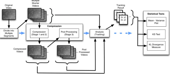
Figure 3.2: Analysis-aware video compression process.
3.2.3 Statistical Tests
Because I judge the quality of a compressed video by comparing its error with that introduced by noise in the original video, the relative distributions should be considered. To provide confidence values, a quantitative approach in preferred. In testing the performance of my methods, I applied two experiments: the two-sample Kolmogorov-Smirnov (KS) test and Kullback-Leibler (K-L) divergence computation.
KS test
confidence threshold in order to make the decision on whether the two MSD samples are from the same distribution.
K-L divergence
Computing a K-L divergence can also compare two samples of MSD values from two unknown distributions. K-L divergence is a concept in information theory that measures the difference between two probability distributions. It can be understood as the information lost when probability distributionsQis used to approximated probability distributionP.
In my experiment,P is the sampled population of the MSD values for the original video and Q is the sampled population of the MSD values for a compressed video. The measurement is
non-symmetric: KL-div(P, Q)is generally different fromKL-div(Q, P). Similar to the KS test, for this test, the scientist also must select a confidence threshold in order to make the decision on whether the two MSD samples are from the same distribution.
3.3 Methods
The basic form of my analysis-preserving method and analysis-aware method both apply a two-step approach.
In the first (segmentation) stage, the analysis-critical regions in every frame in the video are detected. The methods use an approach based on correlation and mathematical morphology to determine the important part of the video in a domain- and analysis-independent manner. Every pixel in every frame is labeled as either foreground or background. This result is stored in a binary map.
For this stage of the analysis-aware algorithm, I designed and evaluated two different variations. They are detailed in 3.3.2. After the compression is completed, the resulting compressed video has a much smaller size, and it is still useful for analysis.
The extended form of analysis-aware compression includes a third stage: The compression may still introduce changes into the analysis result. To address this problem, I designed a post-processing stage to refine the compressed video. The post-post-processing stage makes use of the noise statistics in the video and refines the video by reproducing the noise that matches the video system characteristics as explained in Subsection 3.3.3.
The central problem in the proposed methods is to find the separation between foreground pixels (which may carry information) and background pixels (which contain only noise) in microscopy video.
The background noise in the video can be well modeled by a Gaussian distribution plus a Poisson distribution:
N(0, σ) +P(λ) (3.1)
Importantly, neither of these terms depends on the values of neighboring pixels: they are identically randomly distributed among the pixels in the image (Sheppard et al., 2006).
3.3.1 Segmentation Stage
The goal of segmentation is to accurately detect the regions of pixels in a microscopy video frame that might affect analysis. The analysis-independent method for this task made use of the PSF to remove regions containing only noise as detailed in Subsection 2.6.1.
Figure 3.3: Mathematical morphology portions of the original algorithm: (a) a sub region of the first frame in the original video; (b) the correlation-based segmentation result without refinement; (c) the segmentation result after erosion refinement; (d) the segmentation result after erosion and dilation refinement. Some foreground regions in (d) are due to other beads that move into this region in later frames.
The correlation-based segmentation for detecting moving objects in microscopy video is the same in both analysis-preserving and analysis-aware method. Because of the PSF, every pixel is blended slightly with its neighboring pixels. This means that any moving image feature will have a correlated impact on a region of pixels rather than only a single pixel. This does not hold for shot noise and electronic noise, which scale with image brightness but are uncorrelated between pixels. To get a foreground score for every pixel, the method computes the Pearson’s correlation score between it and its neighbors:
Ri =|
Pk
j=1(xj−x)(y¯ ij −y¯i) kσxσyi
| (3.2)
The method computes this value for all eight neighboring pixels for each pixel. It then computes the maximum of all neighbor scores and use a threshold on this to determine which pixels are in the foreground. The threshold was determined by running multiple passes of bead tracking on the compressed video having the same tracking result as the uncompressed video but it can also be determined for a system with known sensor characteristics based on a likelihood threshold based on the system’s noise characteristics. Once determined, this threshold can be transferred to videos taken with similar experiment setups. After every pixel has a score assigned to it, all pixels whose score are above the threshold and are marked as potential foreground pixels in a binary map.
Figure 3.4 shows the impact on compression size as this threshold is increased; fewer pixels are selected as foreground and the compression ratio improves. However, at some point this causes foreground pixels in the image to be missed, which impacts the data analysis and the compression begins to change the results of analysis. Because there is no general solution to the question “how much change to analysis values is too much”, I stop at this level and I select the threshold that has the best compression without impacting analysis.
This threshold is set to a liberal value to avoid losing actual features, with the result that the map contains many small false-positive pixel groups whose size is smaller than the PSF for a given microscope. The PSF would spread actual features over larger areas, so the method removes these false positives using the mathematical morphology erosion operation (Serra, 1982). Figure 3.3 shows one example of the test video frame image and the result binary map cleaned up by erosion. The resulting cleaned binary map guides compression.
Figure 3.5: Example frame from each of the videos tested, each named as in the description and tables.
In the analysis-preserving method, I perform the dilation size that is equivalent to the erosion size plus additional dilation to expand foreground region in the correlation-based segmentation result. This increased dilation (shown in Figure 3.3) provided a conservative estimation of foreground regions to provide an (analysis-method-dependent) region increase to ensure identical results. In the analysis-aware method, the expanded region is not required, so the additional dilation size is not applied - resulting in a much smaller foreground region and greater compression.
My collaborators evaluate their data using the CISMM Video Spot Tracker (CISMM, 2017). An example of a binary map before refinement and after refinement is given in Figure 3.1.
3.3.2 Compression Stage
The first approach processes the video frames by averaging background pixel values over time and then losslessly compressing the processed video frames using a standard algorithm. The pre-processed video has many pixel locations with constant value over time, which can be efficiently encoded to provide high compression. Tests were done to compare four standard compression techniques and software: bzip2, jpeg2000, H.264 and H.265. The result showed that the three modern compression routines all give a similar good compression with the processed video frames. From these four methods, H.265 and H.264 achieve the smallest two compressed video file size based on my data set. H.265 is 4% smaller compressed video size than H.264 but the encoding speed of H.265 was much slower than other three techniques. Therefore I choose to use H.264 in my algorithm implementations and experiments. The results should apply to any lossless video compressor.