Principal component analyses for tree structured objects

(1)

Principal Component Analyses For Tree Structured Objects

Burcu Aydın

A dissertation submitted to the faculty of the University of North Carolina at Chapel Hill in partial fulfillment of the requirements for the degree of Doctor of Philosophy in the Department of Statistics and Operations Research.

Chapel Hill 2009

Approved by,

Elizabeth Bullitt

Shu Lu

J.S. Marron

Andrew Nobel

Gabor Pataki

(2)

(3)

Abstract

BURCU AYDIN: Principal Component Analyses For Tree Structured Objects (Under the direction of Gabor Pataki and J.S. Marron)

This study is in the relatively new statistical area of Object Oriented Data Analysis, which considers

general data objects (3D images, movies, etc) as the atoms of interest. The focus is on populations of

tree-structured objects. Due to the highly non-Euclidean properties of the binary tree space, replacing

classical analysis ideas with their counterparts in this new environment is a challenging task.

Ideas analogous to Principal Component Analysis (PCA) for trees have been previously developed

based ontree-lines. In this work, numerically fast (linear time) algorithms are developed for PCA based

tree-lines which enable the first large scale data analysis of trees. Our analysis of tree-line PCA has lead

to the invention of improved Principal Component Analyses, based on the new concepts ofk-tree-lines

andtree-curves.

The tree-line analysis results give promising results. However, many tree-lines are required to

ex-plain most of the variation in the data.

The idea of tree-curves directly targets the drawback of tree-lines. However, no polynomial-time

optimal algorithm to find the optimal tree-curves exists. The heuristics developed give results that

explain more variation than was observed previously.

The k-tree-line study is proposed as a bridge between tree-line and tree-curve ideas. Polynomial

time algorithms are sought for this group of problems.

These three different proposed PCA methods are used to conduct a study to compare the three

existing data sets and measure the age effect on each subpopulation within the sets. The advantages and

shortcomings of each method with respect to each other are also discussed in the context of the data

analysis.

The motivating data set of this study is a collection of the brain vessel structures of105subjects.

Due to the inaccuracies in scanning and tracking of these vessels, this data set is known to include a

high amount of noise. A detailed visualization method is proposed in this work to spot the instances that

(4)

List of Tables

2.1 Slope p-values . . . 22

2.2 Slope p-values of 1-lines . . . 30

3.1 The slope p-values for tree-curves . . . 37

4.1 Node explained comparisons . . . 52

4.2 Slope p-value comparisons . . . 55

5.1 Marked instances for correction . . . 61

5.2 Instances modified . . . 62

(7)

List of Figures

1.1 Example MRA Image . . . 2

1.2 3-D image of brain arteries. . . 3

1.3 1st PC or a data set . . . 8

1.4 Subspace of first two PC’s . . . 8

2.1 Toy data set example . . . 10

2.2 Toy tree-line example . . . 12

2.3 Weighted support tree illustrating Theorem 2.1.1 . . . 15

2.4 Support trees of Data Set 1 . . . 17

2.5 Best fitting tree-lines . . . 19

2.6 Scores Scatterplot 1 . . . 20

2.7 Cumulative Scores Scatterplot 1 . . . 21

2.8 Scatterplot of PC1 score versus age. . . 23

2.9 Total number of nodes explained . . . 24

2.10 First two PC’s of Set 3 . . . 26

2.11 Scores Scatterplot Set 3 . . . 27

2.12 Cumulative Scores Scatterplot Set 3 . . . 28

2.13 Projection size vs Age . . . 29

3.1 A toy example curve consisting of10points.. . . 33

3.2 Slope p-values in tree-curves . . . 36

4.1 BB progress . . . 51

4.2 1-line vs. 2-line comparison, Back . . . 53

4.3 1-line vs. 2-line comparison, Left. . . 53

4.4 1-line vs. 2-line comparison, Right . . . 53

4.5 1-line vs. 2-line comparison, Front . . . 54

(8)

5.2 Back tree of subject 55 . . . 59

5.3 Right tree of subject 28 . . . 60

5.4 Back tree of subject 24 . . . 61

5.5 Back subtree of subject 55, corrected . . . 63

5.6 Right subtree of subject 28, corrected . . . 64

(9)

CHAPTER 1

Introduction

1.1 Motivation: The Blood Vessels Problem

The first motivating example for this study comes from a study of Magnetic Resonance Angiography

(MRA) brain images of a set of73human subjects of both sexes, ranging in age from18to72, collected

by Dr. E. Bullitt of the CASILAB (casilab.med.unc.edu). More recently, an improved version of this set

had become available with an addition of34more subjects.

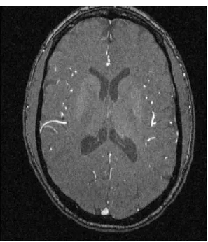
One slice of an MRA image is shown in Figure 1.1. As a distinction from more widely known

MRI, this mode of imaging indicates strong blood flow as white. These white regions are tracked in3

(10)

Figure 1.1: Example MRA Image

Single Slice from a Magnetic Resonance Angiography image for one subject. Bright regions indicate

blood flow.

The set of trees developed from the image of which Figure 1.1 is one slice is shown in Figure

1.2. These figures can be found at (1). Trees are colored according to the regions of the brain. Each

region is studied separately, where each tree is one data point in the data set of its region. The goal

of the present OODA (Object Oriented Data Analysis) is to understand the population structure of107

subjects through4data sets extracted from them. For every subject, the brain vessel structure mainly

consists of four systems that feed the four main areas (back, left, right and back) of the brain. Each of

these systems needs to be analyzed separately. Therefore the vessel data from each subject is divided

into four parts, constituting the four data sets mentioned. These sets are the back data set (gold trees),

(11)

Figure 1.2: Reconstructed set of trees of brain arteries for the same subject as shown in Figure1.1. The colors indicate regions of the brain: Gold (back), Right (blue), Front (red), Left (cyan).

The stored information for each of these trees is quite rich (enabling the detailed view shown in

Figure1.2). Each colored tree consists of a set of branch segments. Each branch segment consists of a

sequence of spheres fit to the white regions in the MRA image (of which Figure1.1was one slice), as

described in Aylward and Bullitt (2002). Each sphere has a center (withx,y,zcoordinates, indicating

location of a point on the center line of the artery), and a radius (indicating arterial thickness).

These reconstructed sets of trees of brain arteries for all subjects are available at Handle(2008).

1.2 Modeling The Data

One big challenge with this data is that it contains too much information to handle at once. One

needs to simplify the structure for meaningful analysis results. The approach taken here is to start out

with considering only variation in thetopologyof the trees, i.e. the branching structure. Other aspects of

the data, such as location, thickness and curvature of each branch are initially ignored. With the removal

of all information other than branching structure, the data turns into four subpopulations ofbinary trees.

The way the binary trees are extracted is as follows: For each of the instances (brain scans), the

back, left, right and front regions are handled separately. Each of these subsystems usually consist of

one main (root) vessel entering the brain from below, and splitting into smaller branches to feed that

region of the brain. The portion of the root vessel until a branch splits off is taken as the root node, and

(12)

procedure is applied at each juncture point. In the end, a binary tree where each vessel trunk between

two split points in the original structure correspond to a node is obtained.

One question at this point is, can a vessel split into three or more branches at a single point? In

this data set splitting into more than two branches is very rare, and these occurrences do not carry

any important implications on structure. Therefore keeping the simple binary structure seems more

important than capturing these rare occurrences. In the cases that this happens, one of the child vessels

is randomly selected as the first one to split off, and the binary tree is created accordingly.

In some of the instances, there can be two root vessels feeding one region and the explained

pro-cedure yields two binary trees. In these cases, for simplicity, one phantom root node is added and the

roots of these two trees are connected to the phantom root node as children, so that a single binary tree

is obtained for each instance in the subpopulations.

There is one set of ambiguities in the construction of the binary trees. That is the choice, made for

each adult branch, of which child branch is put on the left, and which is put on the right. As mentioned

in , the following two ways of resolving this ambiguity are considered here. Using standard terminology

from image analysis, the wordcorrespondenceis used to refer to this choice.

• Thickness Correspondence:Put the node that corresponds to the child with larger median radius

(of the sequence of spheres fit to the MRA image) on the left. Since it is expected that the fatter

child vessel will transport the most blood, this should be a reasonable notion ofdominant branch.

• Descendant Correspondence:Put the node that corresponds to the child with the larger number

of descendants to the left.

These correspondences are compared in Subsection2.2using tree-line analysis methods.

Other types of correspondence, that have not yet been studied, are also possible. An alternative

approach, suggested by Marc Niethammer, is to use location information of the children in this choice.

E.g. in the back tree, one could choose the child which is physically more on the left side (or perhaps

the child whose descendants are more on average to the left) as the left node in this representation. This

would give a representation that is physically closer to the actual data, which may be more natural for

addressing certain types of anatomical issues.

It should be noted that although the size of a data tree remains the same, the inner structure may

(13)

results may differ from one choice to another. Therefore it is important to make a careful decision when

choosing correspondence, and pick the option which captures most of the important aspects of data.

Throughout this study, more that one data set of brain vessels have been available. These can be

listed as follows:

• Data Set1:This is the first set that had been available for analysis. It consists of73subjects. The

back, left and right vessel subpopulations of this data set are used in analysis. This is because the

source of flow for the front trees is variable, causing confusion in separating the sub-populations.

Due to this problem, the front subpopulation of this set is not studied.

• Data Set 2: Through a careful study by Dr. Alim Ladha, many of the flow identification and

starting point problems present in Data Set1 are solved and34more subjects are added to the

study, constituting Data Set2. The front subpopulation is included in analyses run on this set.

• Data Set 3: It is known that there are still many discrepancies exist in Data Set 2. The data

cleaning methods proposed in Section5.4aim to reduce these problems. The further cleansed set

that is obtained by the methods described in Section5.4is labeled as Data Set3. The final data

analyses are run on this set.

The raw data (as in Figure 1.2) belonging to all subjects is publicly available at the website

Han-dle(2008).

1.3 Background and Related Work

1.3.1 Tree Structure Studies In Literature

Phylogenetics is the study of evolutionary relations among species. To study these relations,

phylo-genetic treesare constructed which represent the evolutionary steps occurred in time. The branches on

these trees are constructed according to the likeliness (common genes, etc) between species. See Li et.

al. (2000) and Holmes (1999) for examples of use of trees in phylogenetics.

Cluster analysis is another important area to be listed. Here, trees are formed to again decide which

objects are closer to each other and thus may be grouped together. Here, each object is a leaf node in

(14)

However, these interior nodes do not have a physical meaning. The studies in cluster analysis are usually

based on forming different cluster trees through different methods and then seeking to do inference. See

Everitt et. al. (2001) and Breiman (1996) for examples.

In the classification and regression tree (CART) analysis, data objects are categorized through a

decision tree. The set of all objects constitute the root node. For each decision rule, (questions asked to

patients, etc.) the set is partitioned into further groups (child nodes) according to the responses to that

decision rule. See Breiman et. al. (1984) for a detailed study of this group of trees.

These areas listed are interested in building a particular tree to explain relations between various

objects. They do not focus on the population analysis of a set of trees. Another area, in which

statis-tical analysis of such populations are of interest is medical imaging. Shape analysis of various objects

obtained through medical scanning images is a prominent area on OODA research.

An important shape representation class ism-reps. M-reps capture shape by dividing it into coarse

or fine parts, each of them containing various information (location, radius and angles) in the form of

feature vectors. M-reps provide a good shape representation for shapes that are not far from convex. For

more information on the method, see Pizer et. al. (1999) and the MIDAG web-site.

When the objects to be analyzed are close to convex, carrying the differences into feature vectors and

run a comparative analysis of these vectors (as in M-reps) is a powerful approach. Same methods will

work when objects are further from convexity, but the members of the population have an underlying

common structure. An example to this is a population of human hands (See Haonan Wang’s 2003

dissertation for the details of this example). Although the shape of a hand is very far from convex, all

hands have a common structure consisting of a palm and the five fingers. Each of these components can

e represented by an m-rep and the results can be collected in one vector, enabling the classical statistical

methods to be run on the data.

When the data present different structures from instance to instance, this approach will not be useful.

In our motivating example, the brain vessel trees do not necessarily have same number of vessel trunks.

It is not possible to match one vessel in one instance with another vessel in another subject’s brain as

the corresponding vessel, and make a comparison. Although all parts of the brain are fed with similar

systems for each instance, the exact branching structure that achieves this changes from person to person.

Therefore, an approach which focuses on underlying graph-theory based structures is needed instead of

(15)

Another approach in analyzing tree structured populations is kernel methods, widely used in pattern

analysis. This approach is based on mapping complex structured objects into a high dimensional feature

space, which is Euclidean. Usually finding the exact corresponding point on the feature space for each

data point is hard, so, the idea ofkernel functions is used instead. This function computes the inner

products of each pair of data points in the feature space instead of finding the coordinates themselves,

and statistical analysis is run through these inner products. For more information on these methods, see

Shawe-Taylor and Christianini (2000).

1.3.2 Principal Component Analysis

One of the most common methods used to analyze high dimensional data sets is Principal

Compo-nent Analysis. In its most general sense, Principal CompoCompo-nents are directions that explain structure in

data. In this research, finding the analogues of classical Principal Component Analysis (PCA) plays an

important role, so the main ideas will be explained before going into its counterparts in this research.

PC analysis is introduced by K. Pearson in his1901paper, in which he aimed to find lines and planes

that best fit a set of points inp-dimensional space. The next important work given on the subject was

Hotelling (1933), in which Hotelling aimed to find a smaller (< p) fundamental set of independent

vari-ables that maximize their successive contributions to the total of the variances of the original varivari-ables.

He also introduced the term ”Principal Components”. To further follow the historical development of

PCA ideas, see Girshick (1936,1939), Rao (1964), Gower (1966), Jeffers(1967) and Preisendorfer et.

al. (1988).

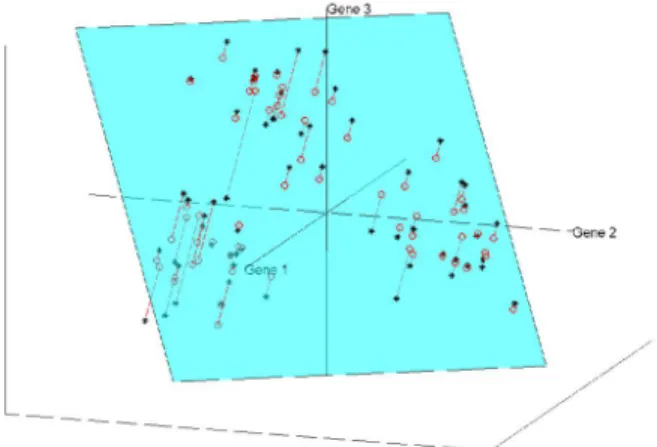
PCA seeks a basis of the space, where the data reside, such that the vectors of the basis explain a

maximal amount of variation in the data. As a first step, a direction vector, where the greatest variation

is achieved when the data points are projected onto it, is calculated. This direction is called the First

Principal Component, and it explains the maximum amount of variation possible in one dimension. An

example can be seen in Figure1.3. Both Figures1.3and1.4can be found in lecture notes web site (34)

(16)

Figure 1.3: First Principal Component of a three dimensional data set, with data points projected onto it.

On second and subsequent steps, the most important directions of variation are sought again, but the

vectors defining them are required to be orthogonal to those identified previously. The result at thekth

step is called thekthPrincipal Component. The Second Principal Component of the previous example

is illustrated in Figure1.4.

(17)

Let d denote the dimension of the original space the data is in. By taking the first k Principal

Components (k < d) and projecting the data set onto the subspace defined by them, one can obtain a

simplified picture of the data where the most important aspects of the variation are kept and some of the

noise is eliminated. Moreover, conducting an analysis of the correlation between each mode of variation

and external parameters becomes possible.

The method to find these directions for data in Euclidean space is very well-known: See Jolliffe

(2002) and Muirhead (1982). The job of carrying the ideas defined in Euclidean space onto the binary

tree space and coming up with an analogous method was first tackled by Wang and Marron (2007). Their

work includes defining the binary tree space mentioned and an appropriate metric for it, and coming up

with useful definitions of atree−line, which is an analog of a line in Euclidean space. They also gave

formal definitions of Principal Component lines in binary tree space, but due to the lack of a solution to

the resulting optimization problems, only limited toy examples (three and four node trees, which thus

allowed manual solutions) were used to illustrate the main ideas proposed. These definitions are given

in Section2.2.3.

1.4 Organization

In this research, through a detailed analysis of the underlying optimization problems of tree-lines,

linear time computational methods to solve them are developed. This advancement allowed the first

actual Object Oriented Data Analysis of a production scale data set of a population of tree structured

objects. The results of this analysis are elaborated in Section2.2.

The analysis results for tree-lines gave important insights into the data, however, they also led the to

the understanding that each of the tree-lines found explains too little variation, and one needs to come

up with richer structures to project the data sets on. Ideas related to the research for this purpose are

tree−curvesandk−tree−lines, which are handled in Sections3.3and4.4.2respectively.

Finally, Section5.4 is dedicated to developing a visualization method that will help the reduction

of noise in the motivating data set, the brain vessel structures of105subjects. Due to the inaccuracies

in scanning and tracking of these vessels, this data set is known to include a high amount of noise.

A detailed visualization method is established in this work to spot the instances that require manual

(18)

CHAPTER 2

Tree-lines

2.1 Definitions And Examples

This section starts with the formal definition of a binary tree:

Definition 2.1.1. Abinary treeis a set of nodes that are connected by edges in a directed fashion, which

starts with one node designated asroot, where each node has at most two children.

Using the notationtifor a single tree, let

T ={t1, ..., tn} (2.1.1)

denote a data set ofnsuch trees. A toy example of a set of3trees is given in Figure2.1.

Figure 2.1: Toy example of a data set of trees, T, withn = 3. This will be used to illustrate several issues below.

To identify the nodes within each tree more easily, the level-order indexing method from Wang and

Marron (2007) is used. The root node has index1. For the remaining nodes, if a node has indexω, then

the index of its left child is2ωand of its right child is2ω+ 1.

(19)

The basis of the analysis is an appropriate metric, i.e. distance, on tree space. The common notion

of Hamming distance is used for this purpose:

Definition 2.1.2. Given two treest1andt2, theirdistanceis

d(t1, t2) =|t1\t2|+|t2\t1|,

where\denotes set difference.

It should be noted that the trees are treated as sets of nodes in this definition. This distance function

is shown to bepseudo-metricin Wang (2003).

In literature, there are various functions defined to measure the distance between two trees. It is

possible to go over all subtrees within two trees and take the total count of un-common subtrees as a

distance measure. (See Shawe-Taylor and Cristianini (2000).) For other examples and further references

on tree distance metrics, see M¨uller-Molina et. al. (2009).

One possible shortfall of the distance function defined above is that, all the nodes in data trees have

the same impact on total distance. One can imagine situations where certain nodes (the ones closer to

the root node, or thicker ones, etc.) carry more importance. One possibility is to assign non-negative

weights to each node on the data trees that signify their relative importance. In this case, the distance

function would sum the weights of the nodes that are not in the intersection of the two data trees instead

of simply counting them. Although this possibility was not deeply investigated within the scope of this

work, it was established that this function also is a metric, and Theorem2.1.1will continue to hold with

this metric.

Two more basic concepts are defined below; the notion of support tree has already been shown in

Figure2.1(as the thin blue lines).

Definition 2.1.3. For a data set T, given as in (2.1.1), the support tree, and the intersection tree are

defined as

Supp(T) = ∪n_i₌₁ti

Int(T) = ∩n_i₌₁ti.

(20)

corresponding intersection trees.

The main idea of a tree-line (notion used for one dimensional representation in tree space) is that it

is constructed by adding a sequence of single nodes, where each new node is a child of the most recent

child:

Definition 2.1.4. Atree-line,L ={`₀,· · ·, `m}, is a sequence of trees where`0 is called the starting

tree, and`i comes from`i−1 by the addition of a single node, labeledvi. In addition eachvi+1 is a

child ofvi.

Figure 2.2: Toy example of a tree-line. Each point is obtained by adding one node to the previous point. Starting point (`0) is the intersection tree of the toy data set of Figure2.1.

An example of a tree-line is given in Figure2.2. Insight as to how well a given tree-line fits a data

set is based upon the concept of projection:

Definition 2.1.5. Given a data treet, itsprojectiononto the tree-lineLis

PL(t) = arg min `∈L

{d(t, `)}.

Wang and Marron (2007) show that this projection is always unique. This will also follow from

ClaimA.1.1in SectionA.1, whose characterization of the projection will be the key in computing the

principal component tree-lines, defined shortly.

The above toy examples provide an illustration. Lett1 be the first tree shown in Figure2.1. Name

the trees in the tree-line, L, shown in Figure2.2, as`0,`1,`2,`3. The set of distances fromt1 to each

each tree inLis tabulated as

j 0 1 2 3

d(t1, `j) 7 6 5 4

(21)

Next, an analog of the first principal component (P C1) is developed, by finding the tree-line that

best fits the data.

Definition 2.1.6. For a data set T and a starting point `0, the first principal component tree-line

starting from this point, i.e.P C1, is

L∗₁ = arg min L

X

ti∈T

d(ti, PL(ti))

The Principal Components we defined in binary tree space start from a fixed starting point tree.

Unlike the Euclidean space, the nature of binary tree space requires the first point not to be completely

arbitrary, but a sufficiently small tree that the line growing from it can cover enough variation. The first

natural approach may be using the root node as the starting point, and this is the first approach taken

in this study. However, it was observed that in this case the first principal component follows the path

of leftmost nodes, which are common to all data trees, and thus does not provide any information on

variation. The second approach is to take theintersection treeas the starting point. The nodes in the

intersection tree exist in all of the data trees, and therefore does not contain any variation, and thus seem

to be an ideal starting point. Indeed when this approach was taken, as will be seen in Section2.2, the

1stPC explains the age correlation the best in most cases, as expected.

Another suggestion on this issue is tonotassume the starting point as a fixed tree, but to incorporate

it into the optimization problem. This approach is not taken in this study, but it may lead to some

interesting results. Although a detailed study is not done for this new problem, it is conjectured that

the optimal solution in this case will use themedian treeas the starting point. See Wang(2003) for a

detailed discussion of the median tree.

In this problem the last point on the first PC does not have any restrictions as the first point does.

However, extending it beyond the nodes in support tree will not result in any gain in the objective

function, but it will not cause any loss either. Therefore, in theory, there are infinitely many optimal

tree-lines for this problem that extend beyond the support tree, but these are useless in practice, so we

take the smallest of these (the one contained in support tree) and use it for our analyses.

In conventional Euclidean PCA, additional components are restricted to lie in the subspace

orthog-onal to existing components, and subject to that restriction, to fit the data as well as possible. For an

(22)

to be defined.

Definition 2.1.7. Given tree-lines L1 = {`1,0, `1,1, . . . , `1,p1}, . . . , Lq = {`q,0, `q,1, . . . , `q,pq}, their

unionis the set of all possible unions of members ofL1throughLq:

L1∪ · · · ∪Lq = {`1,i1 ∪ · · · ∪`q,iq|i1∈ {0, . . . , p1}, . . . , iq∈ {0, . . . , pq}.}

Given a data treet, the projection oftontoL1∪ · · · ∪Lqis

PL1∪···∪Lq(t) = arg min

`∈L1∪···∪Lq

{d(t, `)}. (2.1.2)

In the non-Euclidean tree space, at the present time there is no readily available notion of

orthogo-nality is present, so instead the2nd tree-line is just required that it fits as much of data as possible when

used in combination with the first, and so on.

Definition 2.1.8. Forj ≥1thejth principal component tree-line is defined recursively as

L∗_j = arg min L

X

ti∈T

d(ti, PL∗1∪···∪L∗j−1∪L(ti)), (2.1.3)

and it is abbreviated asP Cj.

For the concept of PC tree-lines to be useful, it is of crucial importance to be able to compute them

efficiently. Another notion to explain the computations will be needed:

Definition 2.1.9. Given a tree-line

L={`0, `1,· · ·, `m}

Define thepath ofLas

VL=`m\`0.

Intuitively, a tree-line that well fits the data “should grow in the direction that captures the most

information”. Furthermore, the jth PC tree-line should only aim to capture information that has not

been explained by the firstj−1PC tree-lines. This intuition is made precise in the following theorem,

(23)

Theorem 2.1.1. Letu0be an exogenously defined starting point,j ≥1, andL∗1, . . . , L∗j−1be the first

j−1PC tree-lines. Forv∈Supp(T)define

wj(v) =



 

 

0, ifv∈VL∗

1 ∪ · · · ∪VL∗j−1,

P

i=1..nδ(v, ti), otherwise

(2.1.4)

Then thejth PC tree-lineL∗_j is the tree-line whose path maximizes the sum ofwj weights in the support

tree, i.e.P

v∈V∗

Lj wj(v).

Here, thedeltafunctionδ(v, ti)is equal to1ifvis a node that exists in treeti, and0otherwise. The

proof of Theorem2.1.1is given in AppendixA.1.

This theorem also points out that, even when we are considering the tree-lines contained in support

tree only, the optimal tree-lines may not be unique. There may be more than one paths extending from

the starting point tree and have the same sum of weights. In this case the selection is made arbitrarily.

Figure2.3 is an illustration: the weight of a node is the number of times the node appears in the

trees of Figure2.1. The black edge is the intersection tree of the same data set. The maximum weight

path attached toInt(T)is the red path, which gives rise to the tree-line of Figure2.2, which is thus the

first principal component of the data set of Figure2.1.

Figure 2.3: Weighted support tree illustrating Theorem2.1.1

After setting the weights of the nodes on the red path to zero, the maximum weight path attached

to Int(T) becomes the green path, which by Theorem2.1.1gives rise toP C2. The usefulness of these

(24)

2.2 Data Analysis Results

This section describes an exploratory data analysis of the three data sets discussed above using the

tree-line ideas. The principal component tree-lines are computed as defined in Theorem 2.1.1. For

Data Set1only, both correspondence types, defined in Section1.2are considered and compared. The

data analysis methodology is explained in detail on Data Set1in Section2.2.1. Next, the comparative

results of all data sets are presented in Section2.2.2. Finally, data analysis conclusions are summarized

in Section2.2.3.

2.2.1 Data Set1

The different brain location types (shown as different colors in Figure1.2) are analyzed as separate

populations (i.e. the blue trees are first considered to be a population, then the gold trees, etc.), called

brain location sub-populations. Partitioning the vessel system in this way reveals some interesting

(25)

Figure 2.4: Support trees of Data Set1, for both types of correspondence (shown in the rows), and for three brain location tree types (shown in columns, corresponding to the colors in Figure1.2). Shows that the descendant correspondence gives a population with more compact variation than the thickness correspondence.

First, the two types of correspondence defined in Section1.2are compared using the concept of the

support tree. This is done by displaying the support trees for each type of correspondence, and for each

of the three tree location types (shown with different colors in Figure1.2), in Figure2.4. Note that all

of the support trees for the descendant correspondence (bottom) are much smaller than for the thickness

correspondence (top), indicating that the descendant correspondence results in a much more compact

population. This seems likely to make it easier for the PCA method to find an effective representation

of the descendant based population.

Figure2.4already reveals an aspect of the population that was previously unknown: there is not a

very strong correlation between median tree thickness of a branch, and the number of children.

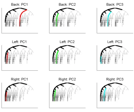
Figure 2.5 shows the first 3 PC tree-lines in Data Set 1, for the three sub-populations (shown as

rows), with the intersection tree as the starting tree, for the descendant correspondence.

(26)

immediately splits into two main trunks, supplying the back sides of the left and right hemispheres.

These two parts of the back circulation are expected to be approximately mirror-image symmetrical

with both sides containing one main vessel and other branches stemming from that. Consequently, for

each tree on the back data set, if a vertical axis that goes through the root node is imagined, the subtrees

on both sides of the axis are expected to be symmetrical with each other.

The results of this model for the back subpopulation are consistent with this expectation. The main

vessel of one of the hemispheres can be seen in the starting point (intersection tree) as the leftmost set

of nodes, while the other main vessel becomes the first principal component.

As for the left and right circulations (cyan and blue trees) of the brain, they are expected to be

close to mirror images of each other. Unlike the case of the back subpopulation, in each of these

circulations there is a single trunk from which smaller branches stem. For this reason the bilateral

symmetry observed within the back trees is not expected to be found here.

The fact thatP C1’s for left and right subpopulations are at later splits suggest that the earlier splits

tend to have relatively few descendants. The remainingP C2andP C3tree-lines do not contain much

additional information by themselves. However, when PC’s1,2and3are considered together and the

left and right subpopulations are compared, i.e. the second and third rows of Figure2.5, the structural

likeliness is quite visible.

It should also be noted that for both of the subpopulations all PC’s are on the left side of the root-axis,

(27)

Figure 2.5: Best fitting tree-lines for Data Set1, for different sub-populations (rows), and PC number (columns). Intersection trees are shown in black.

The tree-lines, and insights obtained from them, were essentially similar for the thickness

corre-spondence, so those graphics are not shown here.

Next comes is the study of the tree-line analog of the familiarscores plotfrom conventional PCA

(a commonly used high dimensional visualization device, sometimes called a draftsman’s plot or a

scatterplot matrix). In that case, the scores are the projection coefficients, which indicate the size of the

component of each data point in the given eigen-direction. Pairwise scatterplots of these often give a set

of useful two dimensional views of the data. In the present case, given a data point and a tree-line, the

correspondingscoreis just the length (i.e. the number of nodes) of the projection. Unlike conventional

(28)

Figure 2.6: Scores Scatterplot for the Descendant Correspondence, Left Side sub-population of Data Set1. Colors show age, symbols gender. No clear visual patterns are apparent.

Figure2.6shows the scores scatterplot for the set of left trees, based on the descendant

correspon-dence. The data points have been colored in Figure2.6, to indicate age, which is an important covariate,

as discussed in Bullitt et al (2008). The color scheme starts with purple for the youngest person (age

20) and extends through a rainbow type spectrum (blue-cyan-green-yellow-orange) to red for the oldest

(age72). An additional covariate, of possible interest, is sex, with females shown as circles, males as

plus signs, and two transgender cases indicated using asterisks.

It was hoped that this visualization would reveal some interesting structure with respect to age

(color), but it is not easy to see any such connection in Figure 2.6. One reason for this is that the

tree-lines only allow the very limited range of scores (projection lengths) as integers, where the score is

bounded by the depth of each tree. A simple way to generate a wider range of scores is to project not just

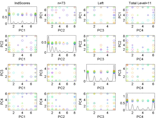
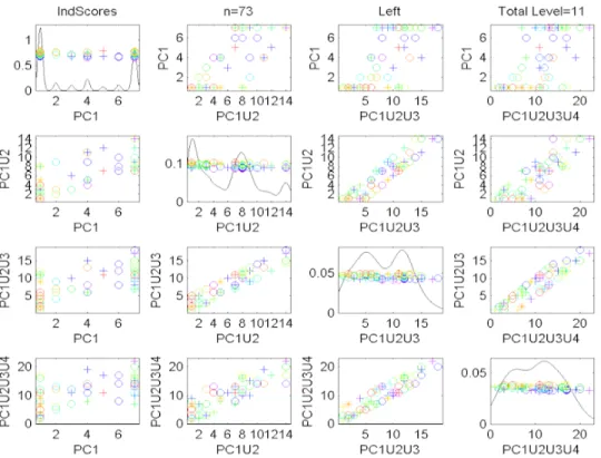
onto simple tree-lines, but instead onto their union, as defined in (2.1.2). Figure2.7shows a scatterplot

matrix, of several union PC scores, in particularP C1 vs. P C1∪2 (shorthand forP C1∪P C2) vs.

P C1∪2∪3vs.P C1∪2∪3∪4. This combined plot, called thecumulative scores scatterplot, shows

(29)

which again is an artifact that follows from each PC score individually having a very limited range of

possible values. This seems to be a serious limitation of the tree-line approach to analyzing population

structure.

As with Figure 2.6, there is unfortunately no readily apparent visual connection between age and

the visible population structure. However, visual impression of this type can be tricky, and in particular

it can be hard to see some subtle effects.

Figure 2.7: Cumulative Scores Scatterplot for the Descendant Correspondence, Left Side sub-population of Data Set1.

Figure 2.8 shows a view that more deeply scrutinizes the dependence of the P C1 score on age,

using a scatterplot, overlaid with the least squares regression fit line. Note that most of the lines slope

downwards, suggesting that older people tend to have a smallerP C1projection than younger people.

Statistical significance of this downward slope is tested by calculating the standard linear regression

p-value for the null hypothesis of 0 slope, which from this on will be calledslopep-value. For the

left tree, using the descendant correspondence, the slope p-value is 0.0025. This result is strongly

significant, indicating that this component is connected with age. This is consistent with the results

(30)

study’s result is the first location specific version of this.

Similar score versus age plots have been made, and hypothesis tests have been run, for other PC

components, and the resulting slopep-values, for the left tree using the descendent correspondence are

summarized in this table:

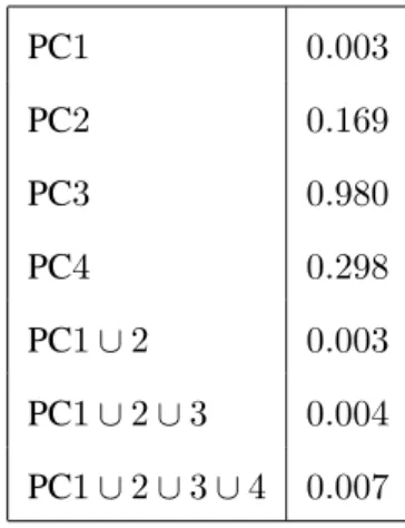
PC1 0.003

PC2 0.169

PC3 0.980

PC4 0.298

PC1∪2 0.003

PC1∪2∪3 0.004

PC1∪2∪3∪4 0.007

(31)

Figure 2.8: Scatterplot ofP C1score versus age in Data Set1. Least squares fit regression line suggests a downward trend in age. Trend is confirmed by the slopep-value of0.0025for Left subpopulation, descendant correspondence.

Note that for the individual PCs, onlyP C1gives a statistically significant result. For the cumulative

PCs, all are significant, but the significance diminishes as more components are added. This suggests

that it is reallyP C1which is the driver of all of these results.

To interpret these results, recall from Figure2.5, that for the left trees,P C1chooses the left child

for the first 3 splits, and the right child at the 4th split. This suggests that there is not a significant

difference between the ages in the tree levels closer to the root, however, the difference does show up

when one looks at the deeper tree structure, in particular after the4th split. This is consistent with the

above remark, that for the left brain sub-population, the first few splits did not seem to contain relevant

population information. Instead the effects of age only appear on splits after level4.

A similar analysis of the back and right brain location sub-populations is done, but none of these

found significant results, so they are not shown here. However, these can be found at the web site (33).

Parallel results for the thickness correspondence are also considered, which again did not yield

(32)

significant results, while thickness never did, is one more indication that descendant correspondence is

preferred. The analyses of the newer data sets (2and3) use descendant correspondence only.

Figure 2.9: Total number of nodes explained, as a function of Cumulative PC Number. Shows that the descendant correspondence allows PCA to explain a much higher proportion of the variation in the population than the thickness correspondence.

One more approach to the issue of correspondence choice is shown in Figure2.9. This shows the

amount of variation explained, as a function of the order of the Cumulative Union PC, for both the

thickness and the descendant correspondences, for the left brain location sub-population. Theamount

of variation explainedis defined to be the sum, over all trees in the sub-population of the lengths of the

projections. There are5023nodes in total for both correspondences. (The correspondence difference

affects the locations of nodes, total count remains the same.)

It is not surprising that these curves are concave, since the first PC is designed to explain the most

variation, which each succeeding component explaining a little bit less. But the important lesson from

Figure2.9is that the descendant correspondence allows PCA to explain much more population structure,

(33)

2.2.2 Comparisons Among Data Sets

Up to this point, using Data Set 1, the difference between the two correspondence types are

inves-tigated, and descendant correspondence is found to be a more compact representation of the data. The

visual structures of the first three principal components are examined and important results on

symme-try are observed. The scatterplots of principal component’s projection lengths are studied, but visual

patterns could not be found.

Similar properties also can be found in Data Sets2and3as shown in this section.

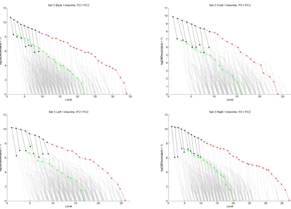
The first two principal components of all subpopulations of Data Set 3 are shown in Figure2.10.

The maximum depth of data trees in this set (37) is much larger than those in Data Set1(11), rendering

the visualization technique used in Section2.2.1impossible for this set. That technique requires the

locations of each possible node for the maximum depth to be allocated on the graph area. For Data

Set1,211points can be allocated beforehand, but for Data Sets2and3the requirement goes up to237

which is unmanageable. A new visualization, more appropriate for trees of greater depth, is developed

for these sets. On these graphs the coordinates of each node displays its number of descendants (vertical

axis) and its level on the binary tree (horizontal axis). For a compact summarization, the logarithm with

base2of the descendant count is the y-axis. Some fine details and refinements of this visualization will

(34)

Figure 2.10: The first two principal components in Data Set3. Grey nodes are support tree, black nodes the intersection tree, red nodes are PC1’s path and green nodes are PC2’s path.

The lines belonging to Data Set2are very similar to these so they are not given here.

A careful comparison of Figures2.5and2.10reveals that the same structural properties observed in

Data Set1, such as higher symmetry in the Back sub-population, also exist in Data Set3. An additional

insight obtained from the Data Set3plots is that the same symmetry property observed in the Back

sub-population also exists in the Front. This result is be expected since the Front sub-sub-population consists of

vessels feeding both the left and right hemispheres of the brain. However this was not be observed in

Data Set1because the Front sub-population data was too unreliable in that set.

The Right and Left sub-populations in Figure2.10lack axial symmetry, but they have the same first

and second principal component structure. These systems are expected to be roughly mirror images of

each other. The observed structure found by principal components is consistent with that expectation.

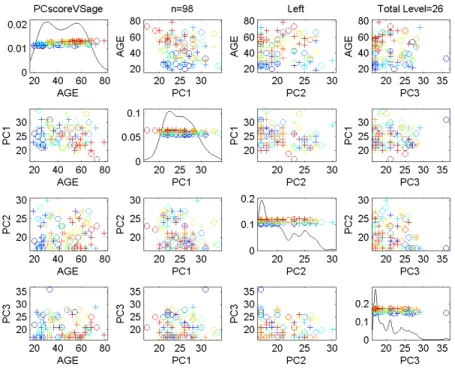
Next, the score scatter plots, similar to Figures2.6and2.7, for the Left sub-population of Data Set

3are given. The scatterplot representations of the results given in Figures2.11and2.12do not yield a

(35)

so they are not shown here.

(36)

Figure 2.12: Cumulative Scores Scatterplot for Left sub-population of Data Set3.

These three data sets come from the same ongoing study, where the last two are improved versions

of Data Set1. Therefore it should not be surprising that basic structural characteristics of the first set

do not change as improvements are made. However, the improvement in one key characteristic is worth

mentioning in detail. The age effect that was observed only in the Left sub-population now becomes

visible in all four sub-populations.

Figure2.13gives an example scatter plot of projection size versus age for the Back sub-population

of Data Set3, PC1. The significant slopep-value (0.016<0.05) is a new result that was not observed

(37)

Figure 2.13: Projection size on PC1 versus age for Back sub-population, Data Set3. Low slopep-value indicates strong dependence.

In fact, the slopep-value summary given in Table2.2demonstrates the major improvement achieved

(38)

Set 1 Set 3 Set 2

Back PC1 * 0.0156 0.0441

PC2 * * *

PC3 * * *

PC4 * * *

PC1U2 * * *

PC1U2U3 * * 0.0283

PC1U2U3U4 * 0.0005 0.0110

Front PC1 - * *

PC2 - * *

PC3 - * *

PC4 - 0.0232 0.0129

PC1U2 - * *

PC1U2U3 - * *

PC1U2U3U4 - 0.0282 0.0202

Right PC1 * 0.0186 0.0178

PC2 * 0.0164 0.0221

PC3 * * *

PC4 * * *

PC1U2 * 0.0002 0.0002

PC1U2U3 * 0.0004 0.0001

PC1U2U3U4 * 0.0002 0.0002

Left PC1 0.003 * *

PC2 * * 0.0490

PC3 * * *

PC4 * * 0.0422

PC1U2 0.003 * 0.0056

PC1U2U3 0.004 * *

(39)

2.2.3 Data Analysis Summary

In summary, there are several important conclusions of this chapter:

• In real data sets with branching structure, tree PCA can reveal interesting insights, such as

sym-metry.

• The descendant correspondence is clearly superior to the thickness correspondence, and is

rec-ommended as the default choice.

• As expected, the back sub-population is seen to have a more symmetric structure.

• The improved Data Sets2and3seem to contain more information because for all sub-populations

there is a statistically significant structural age effect. In particular, the projection size tends to

decrease with age which is consistent with the results of Bullitt (2008).

• There seems to be room for improvement of the tree-line idea for doing PCA on populations

of trees. Other data analytic approaches which allow a richer branching structure within each

(40)

CHAPTER 3

Tree-curves

3.1 Definitions

A tree-curve is a sequence of trees, such that, given a tree in the tree-curve, the next tree in the

sequence is obtained by adding one node. This node has to be a child of existing nodes in the previous

tree to satisfy connectivity requirement. The tree-curve idea is a generalization of the tree-line concept:

the constraint on the location of the next added node is removed from the tree-line definition to obtain

the tree-curve definition. In Euclidean space, all points on a line are required to lie on a single direction.

The constraint on the location of the next added node is considered to emulate this property in tree-lines.

By removing it, a structure considered to be the counter part of a curve in Euclidean space is obtained.

Definition 3.1.1. Atree-curve,C={c₀,· · · , cm}, is a sequence of trees wherec0is called the starting

tree, andcicomes fromci−1by the addition of a single node, labeledvi.

An example tree-curve can be seen in Figure3.1. Note that it starts from an initial tree of two nodes,

and ends at the support tree.

The projection of a data tree onto a tree-curve is the point on the tree-curve with smallest distance

to the data tree:

Definition 3.1.2. Given a data treet, itsprojectiononto the tree-curveCis

PC(t) = arg min c∈C

{d(t, c)}.

(41)

Figure 3.1: A toy example curve consisting of10points.

Definition 3.1.3. For a data setT, thefirst principal component tree-curveis

C₁∗ = arg min C

X

ti∈T

d(ti, PC(ti))

Definition 3.1.4. Forj ≥1thejth principal component tree-curveis defined recursively as:

C_j∗ = arg min C

X

ti∈T

d(ti, PC∗

1∪···∪Cj∗−1∪C(ti)) (3.1.1)

3.2 Heuristics

Unlike the case with lines, the sequence of nodes added to a starting point that define a

tree-curve can be a member of a data tree in any order, as long as connectivity requirement of the points

on the tree-curve is satisfied. So far, this prevented the development of an easy characterization of the

projection of a data tree onto a tree-curve. Moreover, the set of all possible tree-curves on a given

support tree has an order ofO(n!), where n is the number of nodes in the support tree.

As mentioned before, the problem of finding the optimal first principal component have not yet

been has been intractable so far. However, some heuristic methods that give promising results exist. All

heuristics mentioned below are known to give non-optimal results in some cases.

To test their effectiveness, a simulation with 30 randomly generated data sets, each containing 4

(42)

tree-curve can be quickly found using an exhaustive search. The performance of each heuristic is

mea-sured by comparing their resulting tree-curve,C, with the optimal tree-curveC∗ that is found through

exhaustive search. In particular, the performance of a tree-curveCon a data setT is measured with the

following function:

P erf ormance(C, T) = F(C

∗_{, T}₎

F(C, T) ∗100

,

Where F(C, T) is the objective function value that needs to be minimized to reach the optimal

tree-curve:

F(C, T) = X ti∈T

d(ti, PC(ti))

So far following algorithms have been considered:

3.2.1 Weight Order Algorithm (WO)

This algorithm starts from a given starting tree, and adds the nodes from the support tree in the

order of their weights (their number of occurrences in the data set). Ties are broken according to

parent-child relationship when possible: parents are added before their parent-children. This algorithm achieved a

performance measure of98.82.

3.2.2 Greedy Algorithm (G)

Starting from an initial point, at each step the children nodes of the existing nodes in current step are

gone over, and the improvement in objective function if that node is selected to be added is calculated.

The candidate with best contribution is appended to the current tree to obtain the next tree in the curve.

This algorithm gave a performance of89.76.

3.2.3 Switching Algorithm (S)

This method starts from an arbitrary tree-curve, and couples of nodes that bring improvement in the

(43)

The method is terminated when no such couples of nodes remain. This algorithm performed at94.02.

3.2.4 Weight Order + Switching Algorithm (WO+S)

This method combined two heuristics mentioned above, by running the Weight Order algorithm first

and feeding its result to Switching algorithm, to see if any improvement can be achieved over WO result

by simple switching. This has proved to be the best performing method in the simulation with a measure

of99.91, and is used to conduct the data analysis.

3.3 Data Analysis Results

The data analysis has been conducted by running the (WO+S) method, since this one seems to

consistently give the best results. Each data point is projected onto the resulting best fitting tree-curve.

Figure3.2 shows an example of the relation between the size of this projection with the age of each

subject. The red line is fitted to the data using linear regression. This plot is created for all of the

sub-populations available, but none of them seem to present a visual pattern that is different from the others.

Set2, Back sub-population is randomly selected to be shown in Figure3.2, and the rest is omitted from

(44)

Figure 3.2: Size of projection onto tree-curve compared with age for back sub-population. Significant slopep-value proves correlation.

The tree-curve tool yields significant slopep-values for most of the sub-populations available. These

(45)

Set 3 B 0.0285

L 0.0118

R 0.0246

F 0.0500

Set 2 B 0.0067

L 0.0059

R 0.0169

F *

Set 1 B 0.0058

L 0.0184

R *

Table 3.1: The slopep-values obtained by the first principal tree-curve for all data sets. Values more than0.05significance level are shown with *.

The strong significant results obtained using tree-curves prove that this mode of analysis is a

power-ful tool to explain variation in binary trees. In addition, as shown in Figure3.2, the very high projection

sizes obtained renders this tool of analysis an attractive option. Tree-curves seem to capture60%of the

nodes that exist in the data sets. This ratio well exceeds what was obtained in Section2.2by combining

the first 4tree-lines. However, note that for this tool, the length of the projection is not exactly equal

the number of nodes covered by the principal component, as was the case for tree-lines. Due to the

structural nature of tree-curves, some nodes that do not exist in a data tree may appear in its projection.

A major drawback of tree-curves is that, it is hard to visually express the resulting tree-curve of an

analysis run. Each tree-curve contains all the nodes that exist in the support tree, and what differentiates

one curve from another is the sequence of its nodes. Although it is possible to visually express a

sequence in some ways (one can use changing rainbow colors, etc.), visual inspection of those and

trying to infer a structural trend from them is extremely hard. For example, the structure properties

observed using tree-lines (symmetry) is very challenging to infer by using the tree-curve tool.

Another drawback of this method is that, we were unable to solve the resulting optimization

(46)

accuracy can be determined by comparing them to brute force method calculation results, the

(47)

CHAPTER 4

K-tree-lines

So far, the tree-line and tree-curve ideas have been examined in Chapters2.2.3and2.2.3,

respec-tively. The tree-line problem can be solved efficiently. However, the number of nodes that can be

explained by any tree-line of nodes of a data tree is limited to the depth of the data set as pointed out in

Section2.2. Therefore every tree-line explains only a limited amount of variation. Tree-curves seem to

overcome this limitation. The tree-curve considered in Chapter3.3includes60percent of the nodes in

Data Set1. A major drawback of the tree-curve approach is that, a method to find an optimal tree-curve

has not yet been discovered. The data analysis is currently run using heuristic methods. Although these

heuristics are known to give accurate results on small data sets, their performance in large data sets

cannot be accurately measured.

The idea ofk-tree-linesis developed as a bridge between the tree-line and tree-curve concepts. When

constructing a tree-line, each tree is obtained by adding a child to the last node of the previous tree. This

last node, whose children are candidates for addition, is called anactive node. In tree-curves, a child

of any node in the previous tree can be added to get the next element of the sequence. Therefore all

the nodes in the previous tree are active, provided they have un-added children. In a k-tree-line, at each

step, onlyknodes that were added last are active.

The organization of this Chapter is follows: In Section4.1, the definitions of main concepts are

ex-plained. The complexity of thek-tree-line problem is examined in Section4.2. Section4.3is dedicated

to the2-tree-line Branch&Bound Algorithm, which is used to obtain the numerical results elaborated in

(48)

4.1 Definitions

The formal definition of a k-tree-line is:

Definition 4.1.1. Ak-tree-line,K={`₀,· · · , `m}, is a sequence of trees where`0is called the starting

tree, and`icomes from`i−1by the addition of a single node, labeledvi. In addition eachvi+1is a child

of one of the nodes in{v_i−k+1,· · · , vi}, or in the case wherek > i, it is a child of one of the members

of {`0, v1,· · · , vi}. A k-tree-line of which the last k nodes are leaves of the support tree, that is, a

k-tree-line that cannot be further extended is called amaximalk-tree-line. All other lines are called

partialk-tree-lines.

It can be seen that the k-tree-line is a generalization of both problems. Whenk = 1, the tree-line

problem is obtained, whenk=∞, the structure becomes a tree-curve.

The limitation of tree-lines, that they cover too little for each line, can be overcome when larger

k’s are used. The advantage over the tree-curve idea is thatk-tree-lines can be easier to compute while

still yielding a relatively rich structure. It is conjectured that a4or5-tree-line will behave very much

like a tree-curve. While it does not seem to be possible to find an optimal solution to the tree-curve

problem in polynomial time, it may be possible to do so for ak-tree-line problem. The complexity issue

ofk-tree-lines will be discussed in Section4.2.

As before, the projection of a data tree onto a k-tree-line is the point on the k-tree-line with smallest

distance to the data tree:

Definition 4.1.2. Given a data treet, itsprojectiononto the k-tree-lineKis

PK(t) = arg min `∈K

{d(t, `)}.

Unlike the tree-line case, the projection of a data point does not have to be unique.

The principal components are also defined similarly:

Definition 4.1.3. For a data setT, thefirst principal component k-tree-lineis

K₁∗ = arg min K

X

ti∈T

(49)

Definition 4.1.4. Forj ≥1thejth principal component k-tree-lineis defined recursively as:

K_j∗= arg min K

X

ti∈T

d(ti, PK∗

1∪···∪Kj∗−1∪K(ti)) (4.1.1)

4.2 Complexity Of The

2 -Tree-Line Problem

The first step in solving the k-tree-line problem is to determine if a polynomial-time solution exists.

For simplicity, the2-tree-line problem will be handled only.

The approach taken here is to count all possible2-tree-lines on a given support tree. It should be

noted that for a given data set, the number of possible k-tree-lines depends on the size of its support tree

only, and not to the number of data trees in it. In this section, it will be assumed that the support tree is

a full tree, i.e. all levels of the support tree include all the nodes on those levels. Another simplification

is that we will assume the starting tree is the root node. This approach will give an upper bound on the

2-tree-line count, since arranging the same number of nodes in a full tree and starting from the root node

will give the highest number of possible2-tree-lines. These two assumptions will enable us to disregard

the structure of an arbitrary starting tree and the support tree. The exact count of all2-tree-lines would

depend on the structure of the support tree, which will vary from data set to data set, and also it is not

necessary. The aim is to check the problem’s tractability only, and a polynomial upper bound on the

number of possible solutions is sufficient for our purpose.

Lemma 4.2.1. For a data set with a full support tree ofmnodes, the number of all2-tree-lines has an

order ofO(m2.9).

The proof of Lemma4.2.1is in AppendixA.2. This result is used to obtain the following theorem:

Theorem 4.2.1. For a data set with a full support tree ofmnodes, the run time of the brute force method

of listing all possible2-tree-lines has an order ofO(m2.9logm).

Lemma 4.2.1already establishes the order for the total count of 2-tree-lines. To prove Theorem

4.2.1, we also need the maximum length of these2-tree-lines.

The full support tree withmnodes has a depthlog₂(m+ 1). And it is easy to see that the2-tree-line

with maximum number of nodes in it that can be defined on this support tree has1 + 2∗(log₂(m+ 1))

(50)

contain at most 2 nodes from each level, except the root level. Therefore, the maximum number of

nodes contained in each2-tree-line has an order ofO(logm). Combine this with Lemma4.2.1, and we

see that the order of all nodes contained in the list of all2-tree-lines isO(m2.9logm).

The last step needed to prove Theorem4.2.1is to show that the brute force method needs to account

every node on the2-tree-line list only once to form the list. For this, we refer to the Section4.3.2, where

the mechanism of brute force method is described on a small example.

Theorem4.2.1establishes that we have a polynomial time problem with order less than4th_.

How-ever, despite this initial optimistic result, a deeper look at our data sets shows that even the current order

is very hard to compute with the current input size being used in this research.

The smallest data set, Data Set1, has around500nodes on its support tree. This means that5003,

or125billion2-tree-lines need to be stored before searching for the optimal2-line, and this seems to

exceed the current computation capacity of regular personal computers. For that reason, a Branch &

Bound based algorithm is developed to find the optimal2-tree-lines. This algorithm will be elaborated

in the following section.

4.3 A Branch And Bound Algorithm For

2 -Tree-Lines

4.3.1 Background

The basic idea of this family of algorithms is as follows:

Consider the general optimization problemOP:

Minimize G=g(x) Subject to: x∈ F

Where F represents the set of all feasible solutions to the problem OP, and G∗ is the optimal

solution value being sought. Notice that the definition of OP is generic enough so that almost any

optimization problem can be written in this form.

Now suppose that the setF can be divided intonpartitions, where each partition is calledFi _with

i= 1. . . n. Therefore we have:F =F1_∪_{. . .}_{∪ F}n_{. Over these}_n_{pieces of the feasible region, we can}

(51)

Minimize Gi=g(x) Subject to: x∈ Fi

WhereG∗_i are the optimal solution values of the respective problems. Clearly, we can write:

G∗ = min i=1...n{G

∗

i}

The idea of partitioning a bigger problem into smaller portions is calledBranching.

At this stage, we have nsmaller problems to handle instead of the original problem, OP. If the

original problem is hard to solve to optimality, so will be the partition problemsOPi. However, suppose

that we have methods to:

1. Recognize if problemOPi_{has no feasible solution and thus}_Fi₌_∅_.

2. Find at least one feasible pointxi_{f eas}∈ Fi_if_Fi _{is nonempty.}

3. Solve arelaxed version of problemOPi_{, and obtain a point}_xi

rel. This point may or may not be inFi_.

For each of the subproblems with a nonempty feasible region, thexi_{f eas} andxi_relare found. Since

xi_{f eas}is any point inFi_{, we know that}_g(xi

f eas)≥g(xi

∗_{). Also it is clear that relaxation of a problem}

always achieves a smaller or equal objective function value than actual problem: g(xi∗) ≥ g(xi_rel).

Therefore, through these two methods we construct an interval in which the optimal objective function

value resides:g(xi∗)∈[g(xi_rel), g(xi_{f eas})].

Each iteration of the Branch And Bound Algorithm (B&B) starts with finding xi_{f eas} andxi_rel for

each subproblem, or identifying the subproblem to be infeasible. Such cases are excluded from

fur-ther branching. For each of the feasible partitions, the intervals [g(xi_rel), g(xi_{f eas})] are compared.

If one of the intervals is dominated by another, say, for subproblems i andj, [g(xi_rel), g(xi_{f eas})]∩

[g(xj_rel), g(xj_{f eas})] = ∅and g(x_{f eas}i ) < g(xj_rel), then subproblemj and its feasible region Fj _is

re-moved from consideration. This step of finding bounds for each subproblem is calledbounding, and the

removed infeasible or dominated subproblems (or branches) are called to becutorpruned.

At any point during the progress of the algorithm, the smallest lower bound of any of the partitions

(52)

overall upper bound. This bracket gives the interval for the overall optimal objective function value at

any time point.

After all possible cuts are performed, the remaining subproblems are further partitioned according to

a pre-defined method. The B&B terminates when a point inFgets singled out as the optimal solution,

or when a sufficiently small interval for the optimal solution is reached.

4.3.2 2-Tree-Lines Adaptation

Recall the objective function of the first2-tree-line problem:

K₁∗ = arg min K

X

ti∈T

d(ti, PK(ti))

That is, we are looking for a set of ordered nodes to be added to a starting point tree where each

node is a child of one of the two most recently added nodes, or, for the first two added nodes, child of

the starting tree.

Throughout this section, it will be assumed that the starting tree is the root node. The algorithm we

describe is easily adapted to the case where the starting tree is arbitrary, and the adaptation consists of

technical details rather than any enhancement in the theory.

Let us consider the process of listing all possible2-tree-lines. For simplicity, assume that the support

treeST is a full tree with4levels:

ST ={1,2,3,4,5,6,7,8,9,10,11,12,13,14,15}

The counting method developed in AppendixA.2 implies that there are208possible maximal

2-tree-lines on this support tree. To be able to list all of these2-tree-lines, we need to start from the root

node and run an iterative procedure.

Let the list of current partial2-tree-lines at stepibe calledLi. Clearly,L0 ={(1)}, the root node.

At the next step, we look for the nodes that can be used to extend the elements of current list by one

node. ForL1, either node2or node3can be appended to the root node to reach a next level2-tree-line,

Principal component analyses for tree structured objects