METHODS OF ENSEMBLE DATA ASSIMILATION ON ADAPTIVE MOVING MESHES
Colin Guider
A dissertation submitted to the faculty at the University of North Carolina at Chapel Hill in partial fulfillment of the requirements for the degree of Doctor of Philosophy in the Department of
Mathematics in the College of Arts and Sciences.
Chapel Hill 2019
Approved by:
Chris K. R. T. Jones
Amarjit Budhiraja
Alberto Carrassi
Katie Newhall
c 2019 Colin Guider
ABSTRACT
Colin Guider: Methods of Ensemble Data Assimilation on Adaptive Moving Meshes
(Under the direction of Chris K. R. T. Jones)
Numerical models solved on adaptive moving meshes have become increasingly prevalent in recent
years. In particular, neXtSIM is a 2D model of sea-ice that is numerically solved on a Lagrangian
mesh that does not conserve the number of mesh points. In this dissertation, we present two
novel approaches to the formulation of ensemble data assimilation for models with this underlying
computational structure. Specifically, we map ensemble members onto a common reference mesh,
where the Ensemble Kalman Filter (EnKF) can be performed. Numerical experiments are carried
out using 1D prototypical models: Burgers and Kuramoto-Sivashinsky equations, with both Eulerian
and Lagrangian synthetic observations assimilated. One of the approaches is very effective, while
the other is significantly less so.
We also present a novel approach in the formulation of the Local Ensemble Transform Kalman
Filter (LETKF) on a conservative moving mesh model. This is also achieved by mapping the
ensemble members onto a common reference mesh, but it done in a significantly different manner
than from the previous two approaches. Specifically, the common mesh is formed by taking an
equidistributing mesh for the previous output of the algorithm. The preliminary results of this
ACKNOWLEDGEMENTS
First, I would like to thank my advisor, Chris Jones. He took me on as a student at a time when
I was unsure of which direction I wanted to take in my research, and gave me a very interesting
problem that I think has real-world applicability. Chris stuck with me through my ups and downs,
and I really appreciate that.
I would also like to thank my collaborators: Alberto Carrassi, Ali Aydogdu, Matthias Rabatel,
and Pierre Rampal from the Nansen Center; Cassidy Krause and Erik Van Vleck at the University
of Kansas; Nikhil Shankar at the University of Michigan; and John Maclean and Christian Sampson
here at UNC - Chapel Hill. This work would not have been possible without them.
I would also like to acknowledge Colin Grudzien, Paul Cornwell, and Claire Kiers for great
advice given to me along the way.
I want to thank everyone at the Nansen Center in Bergen, Norway for the warm hospitality and
wonderful time I spent there. I would also like to thank everyone here in the math department here
at UNC.
I would like to thank Chris, Alberto, Amarjit, Katie, and Christian for serving on my committee.
TABLE OF CONTENTS
LIST OF FIGURES . . . . ix
LIST OF TABLES . . . . xi
CHAPTER 1: INTRODUCTION . . . . 1
1.1 The Field of Data Assimilation . . . 2
1.2 Adaptive Mesh Refinement . . . 2
1.3 The Problem at Hand . . . 4
CHAPTER 2: DATA ASSIMILATION . . . . 5
2.1 What is Data Assimilation? . . . 5
2.2 Filtering . . . 6
2.3 Derivation of the Kalman Filter . . . 7
2.4 The Ensemble Kalman Filter . . . 9
2.4.1 Stochastic Ensemble Kalman Filter . . . 10
2.4.2 Local Ensemble Transform Kalman Filter . . . 10
2.5 The Particle Filter . . . 11
2.5.1 A Basic Particle Filter . . . 12
2.5.2 A Particle Filter with Resampling . . . 12
2.6 Summary . . . 13
CHAPTER 3: PHYSICAL MODELS ON ADAPTIVE MOVING MESHES WITH REMESHING . . . . 14
3.1 Introduction . . . 14
3.1.1 Adaptive mesh models . . . 14
3.1.2 Data assimilation for adaptive mesh models: the issue . . . 14
3.1.4 Goal and Outline . . . 17
3.2 The physical model and its integration . . . 18
3.3 A one-dimensional, non-conservative, velocity-based adaptive moving mesh . . . 20
3.3.1 The mesh features and its setup . . . 20
3.3.2 The remeshing procedure . . . 22
3.4 The model state and its evolution . . . 23
3.5 The Numerical Models . . . 25
3.6 Summary . . . 27
CHAPTER 4: THE FIRST APPROACH TO THE ADAPTIVE MESH ENKF: INTERPOLATION . . . . 29
4.1 The ensemble Kalman filter for an adaptive moving mesh model . . . 29
4.1.1 Fixed reference meshes . . . 31
4.1.2 Mapping onto a fixed reference mesh . . . 32
4.1.3 Observation operator . . . 33
4.1.4 Analysis using the ensemble Kalman filter . . . 34
4.1.5 From a fixed reference mesh to an adaptive moving mesh . . . 36
4.2 Experimental setup . . . 38
4.3 Results . . . 39
4.3.1 Modified EnKF for adaptive moving mesh models - Burgers’ equation . . . . 39
4.3.2 Modified EnKF for adaptive moving mesh models - Kuramoto-Sivashinsky equation . . . 42
4.3.3 Impact of observation type: Eulerian versus Lagrangian . . . 46
4.4 Conclusions . . . 47
CHAPTER 5: THE SECOND APPROACH TO THE ADAPTIVE MESH ENKF: NO INTERPOLATION . . . . 50
5.1 Introduction . . . 50
5.2 The EnKF for an adaptive moving mesh model - second version . . . 51
5.2.1 The fixed reference mesh . . . 51
5.2.2 Projecting onto the high-resolution fixed reference mesh . . . 51
5.2.4 Analysis using the ensemble Kalman filter . . . 52
5.3 Experimental Setup . . . 55
5.4 Results . . . 55
5.5 Conclusions . . . 58
CHAPTER 6: ADAPTIVE MESH ENKF ON A MOVING REFERENCE MESH 60 6.1 Introduction . . . 60
6.2 Adaptive Mesh Movement in 1D . . . 61
6.3 The Local Ensemble Transform Kalman Filter (LETKF) for a Conservative Adaptive Moving Mesh Model . . . 62
6.3.1 The model state and its evolution . . . 63
6.3.2 Mapping onto a fixed reference mesh . . . 63
6.4 Experimental Setup . . . 64
6.5 Results . . . 65
6.6 Conclusions . . . 66
CHAPTER 7: SUMMARY OF RESULTS AND FUTURE DIRECTIONS . . . . 67
LIST OF FIGURES
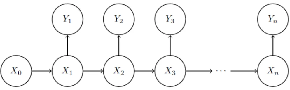
2.1 Dependency structure for nonlinear state space model . . . 7
3.1 A simple illustration of the remeshing process with δ1 = 0.2 and δ2 = 0.5: invalid mesh (a)remove z2(tk) which violatesδ1 (b) and insertz∗(tk) not to violate δ2 (c) 23 3.2 An illustration of adaptive moving mesh over time solving Burgers’ equation until t = 1 on a domain z=(0,1]. In this example, the remeshing criteria are based on δ1 = 0.02 andδ2 = 0.05. There are 40 initial adaptive moving mesh nodes and 27 at t= 1; these are shown in green and red, respectively. . . 24
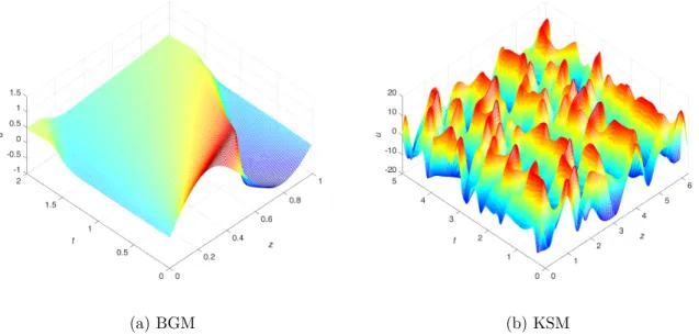
3.3 Solutions of Burgers’ and Kuramoto-Sivasinsky equations. These solutions on a uniform mesh represent the truth from which to sample the observations. Their implementations on an adaptive moving mesh are used as forecast models of the ensemble. . . 27
3.4 Observations sampled from the truth (Fig. 3.3a) in Eulerian(a) and Lagrangian(b) sense mimicking geo-stationary satellite and buoy measurements, respectively. . . 28
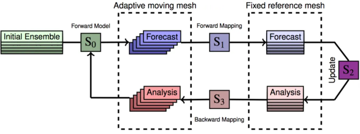
4.1 Illustration of the analysis cycle in the proposed EnKF method for adaptive moving mesh models. In S1, adaptive meshes are mapped onto the fixed reference mesh. The ensemble is updated on the fixed reference mesh at stepS2 (i.e. the analysis). Then, inS3, the updated ensemble members are mapped back to the corresponding adaptive moving meshes. The full process is illustrated in Figure 4.2 for one ensemble member. See text in Sect. 4.1 for full details on the individual process steps S0,S1, S2, and S3. . . 30
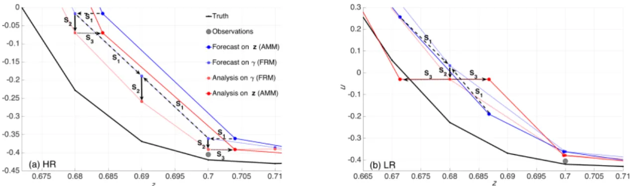
4.2 Schematic illustration of the DA cycle on the high resolution (a)and low resolution (b)fixed reference mesh where onlyuis updated. AMM and FRM stands for adaptive moving mesh and fixed reference mesh, respectively. Dark and pale blue/red lines are forecast/analysis on adaptive moving mesh and fixed reference mesh, respectively. Gray circles are the observations. Following the arrows: S1is the mapping the adaptive moving mesh on to the fixed reference mesh, S2 is the update of the ensemble member, S3 is the backward mapping on the adaptive moving mesh (see Fig. 4.1). . . 37
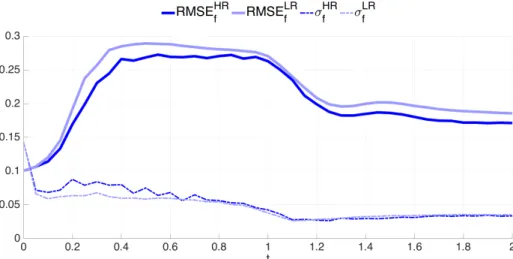
4.3 Time evolution of the forecast RMSE (solid line) and the spread (σ, dashed line) of DA-free ensemble run using BGM. Dark and light lines represent the HR and LR, respectively. . . 40
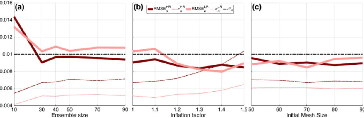
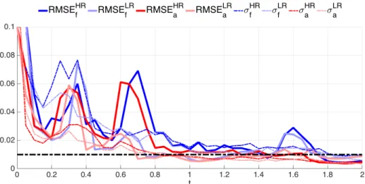
4.4 Time-mean of the RMSE of the analysis ensemble mean (solid line) and ensemble spread (σ, dashed line) of BGM for different ensemble sizeNe (a); inflation factor,α (b); and initial mesh size,N0 (c). Dark and light red show the HR and LR, respectively. 41 4.5 Time evolution of the RMSE (solid line) and spread (σ, dashed line) for BGM until t = 2. Dark and light lines represent the HR and LR, respectively. Blue and red show forecast and analysis, respectively. . . 43
4.6 Same as Figure 4.3 but using KSM. . . 44
4.7 Same as Figure 4.4 but using KSM. . . 44
4.8 Same as Figure 4.5 but using KSM. . . 45
5.1 Plot of forecast and analysis ensemble members at Time = 0.15, after three data assimilation steps. Forecast ensemble members are in green, analysis are in black. . . 55
5.2 Plot of forecast and analysis ensemble members at Time = 0.30, after the fourth data assimilation step. Forecast ensemble members are in green, analysis are in black. We can clearly see here how the analysis overestimates the state along the shock. . . 56
5.3 Plot of forecast and analysis ensemble members at Time = 0.45, after nine data assimilation steps. Forecast ensemble members are in green, analysis are in black. . . 57
5.4 Plot of forecast, analysis, and observation root mean square error. . . 58
6.1 Illustration of projection onto the common mesh for the data assimilation update. Two ensemble members are shown in blue; a common mesh is computed from their ensemble mean, which is shown in red. . . 64
LIST OF TABLES
4.1 Experimental setup parameters: ν is the viscosity, δ1 and δ2 are the remeshing criteria, N1 andN2 the number of nodes in the HR and LR fixed reference mesh,T
the duration of the experiments, ∆tthe analysis interval,dEU L anddLAG0 the number of Eulerian observations and the initial number of Lagrangian observations. . . 39
4.2 Ensemble size (Ne), inflation factor (α), and initial mesh size (N
0) chosen from
the sensitivity experiments in Figure 4.4 to perform the experiment in Figure 4.5. Resulting time mean of the RMSE and spread (σ) for the HR and LR using BGM betweent= 0 and 2 are also listed. . . 42
CHAPTER 1
Introduction
Physical models are ubiquitous in environmental science [1, 2, 3]. They are key in our
un-derstanding of the underlying physical processes; from basic models that can be easily analyzed
and understood, but are drastic simplifications of much more complicated physical phenomena, to
much more complex ones, such as global climate models, that attempt to capture all aspects of
the environment, but are much too large to fully understand. Of course, no matter how complex a
model is, no matter how many parameters it has or how many equations are involved, it will never
be able to perfectly represent the world we observe.
We then turn to the data for more information. With the the rise of big data in the past few
decades, it has become more important than ever to be able to make use of the vast quantity of
information available to us. This is a daunting endeavor: it is difficult to even comprehend the
amount of data available. How can we hope to find even basic patterns in all of this, to find a signal
in the noise? In many fields, like economics and political science, it is quite difficult to understand
the underlying processes. There is a vast amount of data available, but it can be extremely difficult
to find underlying trends.
The advantage in the physical sciences, particular in environmental science and climate, is that
the physics involved is fairly well-understood. This, combined with the wealth of observations of
various aspects of the atmosphere, suggests combining both of these approaches. We can begin
with a physical model, usually a system of partial differential equations, that approximates some
geophysical process like the greenhouse effect [2] or the evolution of a hurricane [4]. Of course, we
have observations of many aspects of these two situations. For example, we have centuries worth
of records of atmospheric carbon and global temperature measurements, and we can look back
at hundreds of past hurricanes to track their paths, precipitation, and wind-speed. Our goal is
to combine these data with our physical models to improve our knowledge of these phenomena.
in the future, whether to project the global average temperature given various emissions scenarios
or to make an informed decision as to which areas to evacuate given a hurricane’s current trajectory.
The field that combines physical models with observations is known asdata assimilation.
1.1 The Field of Data Assimilation
We give a more thorough description of the basic techniques of data assimilation in Chapter 2,
but we give a brief overview here. Generally, the goal is to estimate the value of somestate variable
x, that evolves over time. The problem is that the variablexis not observed, at least not directly. However, we do have some idea of how the state variable evolves over time. This is given by a
state evolution model, denoted by M, which can depend on time and is often represented by a computational solution of a partial differential equation (PDE) model.
While we do not observe x, we do observe a variable y, that has some relationship with x. This relationship is represented by
y=H(x), (1.1)
where His known as the observation operator; this can also depend on time.
A key assumption underlying most situations where data assimilation is applicable is the presence
of noise, both in the state model and observational model. Typically, this noise is taken to be
Gaussian with zero-mean. This is where uncertainty is introduced into the situation, and is what
makes the problem non-trivial. The variance in each of these noise terms is often unknown, but
can be approximated using an ensemble-based process. This is the approach we take throughout.
The problem of estimating the state given observations is fairly straightforward when the state and
observational model are linear; the state models we consider later are exclusively nonlinear. This
raises an issue we can also mitigate using ensemble-based methods.
In the next chapter, we detail the basic probabilistic data assimilation algorithms in use. In
particular, we derive the Kalman Filter, and the Ensemble Kalman Filter (EnKF), its ensemble-based
version. It is the the EnKF that is the basis for the algorithms developed in later chapters of this
work. We also include the particle filter and hybrid filter, for completeness.
1.2 Adaptive Mesh Refinement
Models of the atmosphere and of specific atmospheric processes are generally represented by
so there is no function we can find into which we can plug in the relevant state, location, and time
and which will output the desired quantity. We take a numerical approach to these models. Using
finite difference or finite element methods, we approximate solutions to these systems at various
points in our spatiotemporal domain. For example, Global Climate Models (GCMs) "grid up" the
atmosphere of the Earth into several million evenly distributed points, and the model equations are
solved numerically at these grid points.
Large models are extremely computationally expensive; they must be run on clusters of computers.
This is due to the number of mesh points on which the equations must be solved, in addition to
the quantity of variables and equations involved. It may be desirable to reduce the complexity of
the model in some way to reduce the computational cost needed to effectively run these models.
One approach is to simplify some of the underlying geophysical processes, which would reduce the
number of variables and equations in the model. Another approach, the one that is of interest to
us here, is to find a way to use fewer mesh points. In order to be successful in such a method, we
should strive to place more mesh points in regions of large variation and fewer points in other areas
of the domain. Since the regions of variation will change over time, this leads us to the idea ofmesh
adaptivity.
Some of the existing literature [5] examines the scenario in which the number of mesh points is
fixed in time. The mesh point advection is governed by a computational PDE that the mesh point
velocities must satisfy. However, mesh points are not removed or inserted. For our purposes, we
will refer to such meshes as conservative, in the sense that the number of mesh points is conserved
throughout time. The idea is that the density of mesh points is higher where there is more variation
in the variable(s) of interest, and the points move throughout the process to regions of higher
variation as needed. In the one-dimensional case (we do not consider higher dimensions here), this
is accomplished by equidistributing some function ρ(x), such that its integral between consecutive
mesh points is kept constant. This equidistribution condition can be reformulated as a partial
differential equation that the adaptive mesh points must satisfy.
We will also consider adaptive meshes where the number of mesh points is allowed to change
over time; we refer to such meshes asnon-conservative. In this scenario, the mesh points move over
time, but not according to an equidistribution condition as in the conservative mesh case. This lack
solving the relevant equations. To rectify this, a remeshing process is implemented in regions of
significant distortion in the mesh. In general, mesh points are removed when the distance between
mesh points becomes too small, and mesh points are added when the distance between them becomes
too large. This remeshing process does not preserve the total number of mesh points, a significant
deviation from the conservative case.
1.3 The Problem at Hand
The goal of this dissertation is to develop data assimilation algorithms suitable for adaptive
moving mesh models. Data assimilation in general is discussed at length in Chapter 2. Since
observations are becoming more and more ubiquitous in this age of big data, this is a problem
relevant to several scientific areas, particularly in the geosciences.
Two different situations are considered here. The first is that of a non-conservative adaptive
moving mesh model, such as that employed in neXtSIM. The framework for a non-conservative
mesh in one dimension is developed in Chapter 3. One approach for a data assimilation method is
employed in Chapter 4, and another in Chapter 5. The second is that of a conservative adaptive
moving mesh model. An application of the Local Ensemble Transform Kalman Filter in this scenario
is developed and analyzed in Chapter 6. The main ideas and future directions of this research are
CHAPTER 2
Data Assimilation
2.1 What is Data Assimilation?
The problem of data assimilation can be approached using variational methods or probabilistic
methods. Here, we take a probabilistic approach, since we prefer to construct approximate densities
using an ensemble-based method. In this approach, we will repeatedly apply Bayes’ Theorem to a
prior density for the model and likelihood function to get a posterior density for the model state.
We represent the true state and the observations by a sequence of random variables {(Xn, Yn)}Nn=0
that describe a two-component Markov chain. Thus, at time instant tn,Xnis the true state of the
system and Yn is the observation. We use lower case variables xn, ynto denote realizations of these
random variablesXn,Yn, respectively. Observations are only encountered as realizations of random
variables, so these will always be denoted in lower case. The underlying state process{Xn}Nn=0 is unobservable, so we must conduct all inference based on the observations{Yn}.
Because the state and observation are indexed by time, it is natural to pursue an "online" data
assimilation algorithm; i.e., one that updates the state estimate as new observations come along.
We achieve this using a Bayesian approach.
It will be helpful to simplify the notation. We denote the sets of state variables and observations by
X0:n={X0, X1, . . . , Xn}andY1:n={Y1, . . . , YN}, respectively. We similarly define the realizations of these random variables byx0:n and y1:n. Then an application of Bayes’ Theorem gives
p(x0:n|y1:n)∝p(y1:n|x0:n)p(x0:n). (2.1)
In accordance with the preferred nomenclature,p(x0:n|y1:n) is referred to as the posterior density,
p(y1:n|x0:n) as the likelihood density of the observtionsy1:n given the statex0:n, andp(x0:n) as the prior density.
assimilate the observationynfor eachn. We would also have to calculate the joint likelihood of every
observation Y1:n. Rather than working with joint densities, which would be overly cumbersome, we
formulate the filtering problem, in which natural assumptions regarding the structure of the model
and obserations allows us to rewrite (2.1) so that we can recursively update the probability density
function (pdf) for just the current state Xn at time instanttn, instead of updating the joint density
of X0:n. We then consider more specialized scenarios: we first describe the general Kalman filter,
and then a statistical method known as the Ensemble Kalman Filter (EnKF). Useful versions of the
EnKF include the Stochastic EnKF and the Local Ensemble Transform Kalman Filter (LETKF),
which are both used in the adaptive mesh scenarios discussed in later chapters. Then, we describe a
basic formulation of the Particle Filter.
2.2 Filtering
We make two key assumptions, which are both justified and significantly simplify things. First,
we assume that the distribution ofYngiven{Yk}nk=0−1 andXndepends only onXn. Second, we assume that the distribution of Xn given Xn−1 and {Yk}nk=0−1 depends only on Xn−1. This dependency
structure is shown in Figure 2.1. Given these assumptions, we can rewrite (2.1) as
p(xn|y1:n)∝p(yn|xn)p(xn|y1:n−1), (2.2)
where the forecast density is p(xn|y1:n−1) and the posterior density isp(xn|y1:n). The question of computing the posterior densityp(xn|y1:n) is the filtering problem, and methods that accomplish this task are called filtering methods or filters. In order to compute the forecast densityp(xn|y1:n−1),
one must integrate the posterior density p(xn−1|y1:n−1) from the previous time step, as follows:
p(xn|y1:n−1) = Z
p(xn|xn−1)p(xn−1|y1:n−1)dxn−1. (2.3)
This is the probabilistic analogue of a forecast model in the case of noiseless state dynamics. Once
the forecast density is computed, the posterior density is then:
Figure 2.1: Dependency structure for nonlinear state space model
One advantage the probabilistic approach gives is that a posterior density is obtained, rather than
simply a point estimate. Such estimates of what we term theanalysis xan can be given by the mean
(or other measures of centrality such as the median and mode, depending on the context) of the
posterior densityp(xn|y1:n).
In the general case, we will not be able to produce a closed form expression for the integral in
(2.4). Thus, we cannot obtain such expressions for the forecast and posterior distributions; this
is because the state space models and observation functions will usually be nonlinear. It will be
helpful to begin from a situation in which a closed-form expression can be derived, and from there
progress to more sophisticated scenarios. In the most basic setting we consider, the filter we derive
is known as the classicalKalman Filter.
2.3 Derivation of the Kalman Filter
Suppose that the state-observation Markov process had the dependence structure shown in
Figure 2.1. Further, we suppose that the state model is linear with Gaussian errors; this means we
can write it in the form
Xn∼N(Mnxn−1,Qn), (2.5)
where Xn, xn∈RM and Mn,Qn∈RM×M. In addition, we assume the observations are sampled
independently and with Gaussian errors from the linear observation operatorHn, with
Yn∼N(Hnxn,Rn), (2.6)
where Yn ∈ Rm, Hn ∈ Rm×M, and Rn ∈ Rm×m. Namely, the conditional distribution of
the conditional distribution of Yn given (X0:n, Y0:n−1) is normal with conditional mean HnXn and conditional varianceRn. We assume that the initial state is normally distributed with some background covariance; that is,X0 ∼N(0,B).
It is relatively straightforward to verify that the linear, Gaussian form of the model and
observations imply that the prior, likelihood, and posterior densities in (2.1) are all Gaussian. This
means that we can completely specify each of these distributions by their first and second moments,
i.e., their mean and covariance. To further simplify the notation, we denote the mean of the prior
density p(xn|yn−1) to be xn|n−1 and its covariance by Pn|n−1. Similarly, we denote the mean of
the posterior density p(xn|y1:n) byxn|n and its covariance by Pn|n. This notation refers back to the Bayesian formulation of the filtering problem. The first subscript represents the present time
step, and the second subscript represents the time step of the most recent observation on which
we condition. Using this notation in the model (2.5), we see that the forecast step in the data
assimilation algorithm consists of updating the mean by way of the equation
xn|n−1=Mnxn−1|n−1 (2.7)
and covariance
Pn|n−1 =MnPn−1|n−1MTn +Qn. (2.8)
One can use (2.5) - (2.8), along with Bayes’ Theorem, to determine that the posterior density is
also Gaussian. Its mean and covariance are given by
xn|n=Pn|n
HTnR−t1+Pn−|1n−1xn|n−1
,
Pn|n=HTnRt−1Hn+P−n|1n−1
−1 .
The mean can be rewritten as
xn|n=xn|n−1+Kn
yn−Hnxn|n−1
while the covariance can be written as
Pn|n= (I−KnHn)Pn|n−1, (2.10)
where I is the identity matrix and the matrixKn, known as the Kalman gain, is given by
Kn=Pn|n−1HTn
HnPn|n−1HTn+Rn
−1
. (2.11)
Equations (2.7) - (2.11) fully describe the forecast and analysis cycle for the Kalman filter at time
step n.
2.4 The Ensemble Kalman Filter
The tractability and simplicity of the Kalman Filter has led to its widespread use, even in
scenarios where the model conditions for its validity are not satisfied. One common example of such
a setting is where the linear state modelMnxand linear observation operator Hnx are replaced by general nonlinear functions mn(x) and hn(x), respectively.
One approach to attempt to bypass linearization of the function mn is what is known as the
Ensemble Kalman Filter (EnKF). In this case, one uses the full nonlinear state equation
xn=mn(xn−1) +τn (2.12)
to simulate state values that are used to approximate the forecast density. More specifically, having
obtained a Gaussian approximation for the posterior distribution at time stepn−1, one takesL
samples from this distribution, hereafter labeled as{Xn−1}Li=1. Using this andL realizations
τni
of the state noise, one uses the nonlinear state equation to produce the "forecast ensemble" Xni
according to the equation
Xni =mn
Xni−1
+τni, (2.13)
where i∈ {1, . . . , L}. Assuming a Gaussian forecast density (which may not be valid in the case of a nonlinear model), we can use our forecast ensemble to approximate the mean of the forecast
densitypfn by the sample mean
xn|n−1 =
1
L
L
X
i=1
We approximate the forecast covariance by the ensemble covariance, given by the formula
Pn|n−1
ij = 1
L−1 L
X
i=1
Xni −xn|n−1 Xni −xn|n−1 T
. (2.15)
The forecast distribution is used to produce a Gaussian posterior density by linearizing the observation
function hn and using a modified form of equations (2.9) - (2.10). An alternative to this is to use
an "observation operator-free" version of the EnKF; this will prove useful in Chapter 4.
2.4.1 Stochastic Ensemble Kalman Filter
It turns out that simply using the ensemble-analogues of the Kalman Filter equations for the
analysis step will result in the analysis covariance being underestimated by a factor of (I−KnHn)T. The stochastic Ensemble Kalman Filter provides an adjustment to avoid this difficulty. An instance
of the observational noise is inserted into the update step for each ensemble member. Thus, the
update equations become
Xni|n=Xni|n−1+Kn
yn+ein−HnXni|n−1
, (2.16)
where i∈ {1, . . . , L}. The Kalman gain takes on the expected form, while we have
ein∼N(0,Rn).
As mentioned, adding these noise terms ein ensures that the analysis distribution has the proper
spread. If these noise terms are not added, then the analysis ensemble spread will be too small. We
can then approximate the analysis covariance by
Pn|n= 1
L−1 L
X
i=1
Xni|n−xn|n Xni|n−xn|n
T
. (2.17)
2.4.2 Local Ensemble Transform Kalman Filter
In Chapter 6, we will make use of the Local Ensemble Transform Kalman Filter (LETKF),
introduced by [6]. The main characteristic of this algorithm is that it is a deterministic algorithm,
unlike the stochastic EnKF. Domain localization is used here to reduce the dimensionality of
sufficiently small neighborhoods, and is primarily driven by the dynamics of nearby regions. Using
this assumption, the analysis step is performed using different linear combinations of the ensemble
members in different regions. In this way, a lower-dimensional, less computationally-intensive
analysis can be used to explore a much higher-dimensional space.
The general idea is that the LETKF maps a background ensemble nXni|n−1oL
i=1 to an analysis
ensemble nXni|noL
i=1 by using local observations at time instanttn. We consider an observation of
this system as a triple (yn, hn,Rn), in whichyn is the observation,hn is the (non-linear) observation operator, andRn is the observation error covariance matrix. We assume observations have been truncated to only include those chosen for local analysis. We expect
yn=hn(xn) +n,
where n is a Gaussian random variable with distribution N(0,Rn).
The goal is to infer which state xn produced the observations, and take that as the analysis
mean xn|n. This can be rephrased as minimizing the following cost function
J(xn) =
h
xn−xfn
iT
Cnf−1hxn−xfn
i
+ [yn−hn(xn)]TRn−1[yn−hn(xn)], (2.18)
where Cnf−1 is the inverse restricted to the column space of Cnf, which in turn requires that
xn−xfn is an element of the column space [reference].
We use a modified version of the LETKF throughout our numerical experiments in Chapter 6.
The modifications are designed to produce a useful definition of the analysis mean and covariance,
given the utilization of adaptive mesh refinement.
2.5 The Particle Filter
To avoid relying on the linearity of the observation operator and/or of the state model, or to
avoid using a linearity approximation, we can instead turn to a particle-based method. Here, we
replace the high-dimensional integrals in (2.3) with suitable Monte-Carlo averages. Instead of using
probability densities to describe the distributions we use discrete probability measures supported on
finitely many points. These points and their wights will evolve in time to give the forecast measure
xan by computing an integral with respect to the measure Πn.
2.5.1 A Basic Particle Filter
Suppose that Πn−1 is presented as a discrete probability measure supported on the points n
Xn1−1, . . . , XnL−1owith corresponding weights np1n−1, . . . , pLn−1o. Here,L represents the number of
particles used in each step to approximate the distribution Πn−1. The two key steps in the data
assimilation algorithm proceed as follows:
1. (Prediction Step) We propagate each of the particles Xni−1 →Xˆni using the nonlinear state dynamics (2.12). This requires simulating Lnoise random varialbesτni,i= 1, . . . , L. Given
such random variables, the forecast ensemble members are defined by
ˆ
Xni =mn
Xni−1+τni. (2.19)
Thus, we now have the forecast probability distribution Πfn as a discrete probability measure
concentrated at Lpoints nXˆnioL
i=1 with weights
pin−1
L i=1.
2. (Filtering Step) We update the weights
pin−1 Li=1 using the observation yn at time tn by
setting pin=cpin−1Xˆni, Yn
, where
R(x, y) := exp
−1 2
yn−h
ˆ
XniTR−n1yn−h
ˆ
Xni
. (2.20)
The posterior distribution Πn is then defined as the discrete measure with support points
Xni Li=1 and weights pin .
2.5.2 A Particle Filter with Resampling
The main idea here is to periodically resample from the discrete distribution Πn, with replacement,
to obtain a uniform distribution of weights. Of course, resampling introduces extra noise the
approximating scheme, so it is important not to resample too frequently. We fix a resampling
lag indicator α ∈ N. This parameter specifies the number of time steps between successive resampling steps. Suppose that Πn−1 is given as a discrete probability measure supported on points n
Xn1−1, . . . , XnL−1 o
with corresponding weights np1n−1, . . . , pLn−1 o
. If α does not dividen, then the
probability measure Πn. To do this, we take a random sample of sizeLfrom the discrete distribution
n
Xn1, p1n, . . . ,XnL, pLno
and relabel the new points as
Xn1, . . . , XnL.
The posterior distribution is then given as the discrete distribution on the points nXn1, . . . , XnLo
with all of the weights set equal to 1/L.
2.6 Summary
In this chapter, we introduced the filtering problem and derived the forecast and analysis
distributions given the prior and likelihood distributions. We did this using Bayes’ theorem, which
is fitting due to the probabilistic framework we have chosen. Since the integrals present in these
distributions generally cannot be evaluated analytically, we turn to ensemble-based formulations of
the data assimilation algorithms. In particular, we looked at a basic particle filter with resampling
and two formulations of the Ensemble Kalman Filter: the stochastic EnKF and the LETKF.
One algorithm, not discussed in detail here, used by the author in work on inertial particle
DA is the hybrid particle-ensemble Kalman filter, developed in [7]. The idea here is that certain
models are both high dimensional and very nonlinear. The high dimensionality causes issues with a
standard particle filter, while the nonlinearity and non-Gaussian posterior distributions can lead
a standard EnKF to fail. A hybrid filter will take advantage of each of the individual methods
where appropriate, while avoiding many of the pitfalls. It is shown in [7] that the hybrid filter
performs much better than the EnKF, and about as well as the particle filter, with significantly
fewer particles.
The stochastic EnKF is what we turn to in Chapter 4 and Chapter 5, while we make use of
the LETKF in Chapter 6. These are the algorithms we modify to suit the adaptive moving mesh
problems of interest. However, we must first develop the theory behind adaptive moving meshes,
CHAPTER 3
Physical Models on Adaptive Moving Meshes with Remeshing
3.1 Introduction
3.1.1 Adaptive mesh models
The computational model of a physical phenomenon is typically based on solving a particular
partial differential equation (PDE) with a numerical scheme. Numerical techniques to solve PDEs
evolving in time are most often based on a discretization of the underlying spatial domain. The
resulting mesh is generally fixed in time, but the needs of a given application may require for the
mesh itself to change as the system evolves, adapting to the underlying physics [8]. We consider
here the impact of such a numerical approach on data assimilation.
Two reasons that may lead to the use of an adaptive mesh are: (1) for fluid problems, it is
sometimes preferable to pose the underlying PDEs in a Lagrangian, as opposed to Eulerian, frame,
or (2) the model produces a specific structure, such as a front, shock wave, or overflow that is
localized in space. In case (1), the Lagrangian solver will naturally move the mesh with the evolution
of the PDE [9]. For case (2), the idea is to improve computational accuracy by increasing the mesh
resolution in a neighborhood of the localized structure (see, e.g. [10]). This may be compensated by
the decrease in resolution elsewhere in the domain. Adapting the mesh can prove computationally
efficient in that an adaptive mesh generally requires fewer points than a fixed mesh to attain the
same level of accuracy [5]. Some important application areas where adaptive meshes have been used
are: groundwater equations [11], and thin film equations [12], as well as large geophysical systems
[13, 14].
3.1.2 Data assimilation for adaptive mesh models: the issue
Data assimilation (DA) is the process by which data from observations are assimilated into a
computational model of a physical system. There are numerous mathematical approaches, and
the collection of methods designed to obtain an estimate of the state and parameters of the system
of interest using noisy, usually unevenly distributed, data and an, inevitably approximate, model
of its evolution [16]. There had been considerable development of DA methods in the field of the
geosciences, particularly as a tool to estimate accurate initial conditions for numerical weather
prediction models; a review of the state-of-the-art DA for the geosciences can be found in [17].
Mesh adaptation brings significant challenges to DA. In particular a time-varying mesh may
introduce difficulties in the gradient calculation within variational DA [18]. In an ensemble DA
methodology [19, 20], the challenge arises from the need to compare different ensemble members
in the analysis step. With a moving mesh that depends on the initialization, different ensemble
members may be made up of physical quantities evaluated at a different set of spatial points.
There is another variation that is key to our considerations here, and that is relevant in both cases
described above. The issue is that the nodes in the mesh may become too close together, or too far
apart. Both situations can lead to problems with the computational solver. Some adjustment of
the mesh, based on some prescribed tolerance, may then be preferable, and even necessary. We
are particularly interested in the implications for DA when this adjustment involves the insertion
or deletion of nodes in the mesh. The size of the mesh may then change in time, which has the
consequence that the state vectors at different times may not have the same dimension. In other
words, the state space itself is changing in dimension with time. Consequently, individual ensemble
members, each of them representing a possible realization of the state vector, can even have different
dimensions. In this situation, it is not possible to compute the ensemble-based mean and error
covariances in a straightforward manner, a problem as these are at the core of the ensemble DA
methods [19]. Dealing with and overcoming this situation is the main aim of this chapter and the
following two chapters.
Two specific pieces of work can be viewed as precursors of our methodology. Bonan et al [21]
study an ice sheet that is moving and modeled by a Lagrangian evolution, but without remeshing.
The paper by Du et al. [22] develops DA on an unstructured adaptive mesh. Their mesh is adapted
to the underlying solution to better capture localized structures with a procedure that is akin to
the remeshing in neXtSIM. The challenge we address here is the development of a method that will
3.1.3 Motivation: the Lagrangian sea-ice model neXtSIM
This work is further motivated by a specific application, namely performing ensemble-based
DA for a new class of computational models of sea-ice [23]. In particular, the set-up we develop is
based on the specifications of neXtSIM, which is a stand-alone finite element model employing a
Maxwell elasto-brittle rheology [3, 24] to simulate the mechanical behavior of the sea ice. In this new
rheological framework, the heterogeneous and intermittent character of sea ice deformation [25, 26]
is simulated via a combination of the concepts of elastic memory, progressive damage mechanics, and
viscous-like relaxation of stresses. This model has been applied to simulate the long-term evolution
of the Arctic sea ice cover, with significant success when compared to satellite observations of sea ice
concentration, thickness, and drift [24]. It has also been recently shown how crucial this choice for
the ice rheology is in order to improve the model capabilities, e.g., to reproduce sea ice trajectories.
This makes neXtSIM a powerful research numerical tool, not only to study polar climate processes,
but also for operational applications; e.g., to assist search and rescue operations in ice-infested
waters in the polar regions [27].
neXtSIM is solved on a 2-dimensional unstructured triangular adaptive moving mesh based on
a Lagrangian solver that propagates the mesh of the model in time along with the motion of the
sea ice [28]. Moreover, a mesh adaptation technique, referred to asremeshing, is implemented. It
consists of a local mesh adaptation, a specific feature offered by the BAMG library that is included
in neXtSIM (http://www.ann.jussieu.fr/hecht/ftp/bamg/bamg.pdf). The advantages of a local
mesh modification is that it is efficient, introduces very low numerical dissipation [29], and also
allows local conservation [30]. The remshing algorithm operates on the edges of the triangular
elements to avoid tangling or distortion of the mesh, as well as inserting, or removing, nodes on
the mesh in case it is needed to prevent exceedingly sharp refinements resulting in an excessive
computational burden.
The specific DA methodology we develop for adaptive mesh problems is driven by the
consider-ations of neXtSIM. The remeshing in neXtSIM, and the consequent change in the state vector’s
dimension, is addressed in our assimilation scheme by the introduction of a reference mesh. The
latter represents a common mesh for forming the error covariance matrix from the ensemble members.
The question then arises as to whether this common mesh is used to propagate each individual
the reference mesh, common to all members, could throw away valuable physical information. In
fact, the use of a Lagrangian solver in neXtSIM assures that the mesh configurations are naturally
attuned to the physical evolution of the ice. For this reason, we make the critical methodological
decision to map back to the meshes of the individual ensemble members after the assimilation step.
The Lagrangian solver in the model is thus the primary determinant of the mesh configuration used
in each forecast step. The reference mesh is only used in a temporary capacity to afford a consistent
update at the assimilation step.
3.1.4 Goal and Outline
In this chapter, we proceed towards constructing a 1-dimensional setup designed to capture the
core issues that neXtSIM presents for the applications of an ensemble-based DA scheme. We perform
experiments using both Eulerian (where the observation locations are fixed) and Lagrangian (where
observation locations move with the flow) observations. We test the strategy for two well-known
PDEs: the viscous Burgers and Kuramoto-Sivashinsky equation, whose associated computational
models we refer to as BGM and KSM, respectively. The Burgers’ equation, which can be viewed as
modeling a one-dimensional fluid, is a canonical example for which a localized structure, in this
case a shockwave, develops and an adaptive moving mesh will get denser near the shock front. The
Kuramoto-Sivashinsky equation exhibits chaotic behavior and this provides a natural test-bed for
DA in a dynamical situation that is very common in physical science, and particularly in the DA
applications in the geosciences (see Section 5.2 of [17]).
Our core strategy is to introduce a fixed reference mesh onto which the meshes of the individual
ensemble members are mapped. A key decision is how refined the fixed reference mesh be made.
There are two natural choices here: (a) one that has at most one node of an adaptive moving mesh
in each of its cells, or (b) a reference mesh in which any adaptive moving mesh that may appear has
at least one node in each cell of the fixed reference mesh. We refer to the former as ahigh-resolution
fixed referenced mesh (HR) and the latter a low-resolution fixed reference mesh (LR). A natural
guess would be that the high-resolution mesh will behave more accurately. Although this turns out
to generally be ture, we will show that the low-resolution mesh may result in a better estimate
when the ensemble is appropriately tuned.
There have been other recent studies aimed at tackling the issue of DA on adaptive and/or
variational DA framework. [21] extended the study and provided a comparison between a three
dimensional variational assimilation (3D-Var) [] and an ensemble transform Kalman filter (ETKF)
[]. The mesh they use adapts itself to the flow of the ice-sheet but, in contrast to our case, the total
number of nodes on the mesh is conserved.
[22] approach the issue in an ensemble DA framework using a three dimensional unstructured
adaptive mesh model of geophysical flows [14, 32]. They adopt a fixed reference mesh on which
the analysis is carried out. Each ensemble member is interpolated on a fixed reference mesh
conservatively using a method called supermeshing developed in [33]. In [34], a similar methodology
is used for a tsunami application which exploits adaptive mesh refinement on a regular mesh. Instead
of using a fixed reference mesh, they use the union of meshes of all the ensemble members to perform
the analysis. In summary, [21] addresses the issues that arise with a Lagrangian solver without any
remeshing, whereas the approach in [22] is developed for a model that has the remeshing as part
of its numerical algorithm, but uses an otherwise static mesh. The numerical solver underlying
neXtSIM has both features and thus requires a methodology that differs from these two approaches.
This work thus goes beyond existent works in developing a scheme that addresses the case of a
moving mesh with non-conservative mesh adaptation.
In this chapter, we detail the problem of interest, describe the nature of the adaptive moving
mesh methodologies in one dimension, and describe a remeshing process that is implemented
intermittently. We also describe the model state and its evolution on the adaptive, non-conservative,
1D mesh. In Chapters 4 and 5, we introduce the EnKF using an adaptive moving mesh model in
two different ways.
3.2 The physical model and its integration
This and the following chapters focus on a physical model describing the evolution of a scalar
quantity u (e.g. the temperature, pressure, or one of the velocity components of a fluid) on a
one-dimensional (1D) periodic domain [0, L). We assume that a model of the temporal evolution of
u is available in the form of a partial differential equation
∂u
∂t =f u, ∂u ∂z, . . . ,
∂iu ∂zi, . . .
!
with initial and boundary conditions
u(t0, z) =u0(z), u(t,0) =u(t, L), (3.2)
and withf being, in general, a nonlinear function. Realistic models of geophysical fluids incorporate
(many) more variables, and expressed as a coupled system of PDEs. A notable example in the
field of geosciences, and fluid-dynamics in general, is the system of Navier-Stokes equations; the
fundamental physical equations in neXtSIM have the same form [24]. In this work, we consider the
simpler 1D framework as a proxy of the 2D one in neXtSIM but, as will be made clear below, we
formulate the 1D problem to capture many of the key numerical features of neXtSIM. Some of the
challenges and issues for the higher dimensional case are discussed later.
Solving (3.1) numerically, with initial and boundary conditions (3.2), would usually involve
the following steps: first, discretizing the original PDE in the spatial domain (e.g. using a central
finite difference scheme), and then integrating, forward in time, the resulting system of ordinary
differential equations (ODEs) using an ODE solver (e.g. an Euler or Runge Kutta method). The
standard approach to numerically solving a PDE is appropriate when it is cast in an Eulerian
frame. A key point about neXtSIM, however, is that it is solved in a Lagrangian frame. The use
of a Lagrangian solver is a particular case of a class of techniques that is known as velocity-based
methods in the adaptive mesh literature (see e.g. [9], and references therein). The dynamics of the
adaptive mesh are given, in this case, by usingu coming from the PDE (3.1) as the velocity field for
the mesh points. [5] gives a comprehensive and detailed treatment of the case of adaptive meshes.
A further key feature of neXtSIM as a computational model is that it incorporates a remeshing
procedure. As a result, it is different from the usual problems considered in the adaptive mesh
literature [? ]. In particular, it entails that, in general, no mapping exists from a fixed mesh to the
adaptive mesh that is continuous in time. We call such an adaptive meshnon-conservative as the
number of mesh points will change in time. It is this characteristic that we see as presenting the
greatest challenge to a formulation of DA for neXtSIM, and addressing it in a model situation as
the main contribution of this work, and one that makes it stand apart from previous work in the
3.3 A one-dimensional, non-conservative, velocity-based adaptive moving mesh 3.3.1 The mesh features and its setup
We build here a 1D periodic adaptive moving mesh that retains the key features of neXtSIM’s
2D mesh in being Lagrangian and including remeshing.
For a fixed time, a mesh is given by a set of points{z1, z2, . . . , zN} with eachzj ∈[0, L). Thezj are referred to as the mesh nodes, or points, and we assume they are ordered as follows:
0≤z1<· · ·< zj <· · ·< zN < L. (3.3)
To guide the remeshing, we define the notion of a valid mesh in which the mesh nodes are neither
too close nor too far apart. To this end, we define two parameters: 0 < δ1 < δ2 < L. A mesh
{z1, z2, . . . , zN} is a valid mesh if:
δ1 ≤ |zj+1−zj| ≤δ2 for all j∈N: 1≤j < N−1, and δ1≤ |1+L−zN| ≤δ2. (3.4)
It is further assumed thatδ2/δ1 ≥2 and thatδ2andδ1are both divisors ofL. The former hypothesis is related to the remeshing procedure and will be discussed in Section [], while the latter is useful in
our DA approach and will be discussed in Section []. When condition (3.4) does not hold, the mesh
is called an invalid mesh.
The mesh will evolve following the Lagrangian dynamics associated with the solution of the
PDE (3.1). Eachzj will therefore satisfy the equation
˙
zj =u(t, zj), (3.5)
where ˙=dtd, and u(t, zj) is the velocity. The physical model (3.1), together with the mesh model
(3.5), constitute a set of coupled equations that can be solved either simultaneously, or alternately
[5]. In the former case, the mesh and physical models are solved at the same time, which strongly
ties them together. A drawback of the simultaneous numerical integration is that the larger coupled
system of equations arising by joining the mesh and the physical models is often more difficult to
The neXtSIM model adopts an alternative strategy that bases the prediction of the mesh at
time t+ ∆t, where ∆t is the computational time step, on the mesh and the velocity field at the
current time, t, and then subsequently obtain the physical solution on the new mesh at timet+ ∆t.
As a consequence, the mesh is adjusted to the solution at one time-step earlier. This can cause
imbalance, especially for low-resolution time discretization and rapidly changing systems, but it
offers the advantage that the mesh generator can be coded as a separate module to be incorporated
alongside the main PDE solver for the physical model. This facilitates the possible addition of
conditions or constraints on the mesh adaptation and evolution. Having this ability is key to the
remeshing procedure in neXtSIM.
In neXtSIM, the coupled system, which includes the mesh and the physical model, is solved
in three successive steps: (1) The mesh solver is integrated to obtain the mesh points att+ ∆t
based on the mesh and the physical solution at timet; (2) It is then checked whether the new mesh
points satisfy the requisite condition and, if not, the remeshing procedure is implemented; (3) The
physical solution is then computed at timet+ ∆ton the (possibly remeshed) mesh att+ ∆t.
In the first step, the movement of the mesh nodes is determined by the behavior of the physical
model, which is a special case of the mesh being adaptive. In particular, the dynamics of the physical
model can lead to the emergence of sharp fronts or other localized structures. These features can
then be better resolved through the finer grid that now covers the relevant region, which is the usual
motivation behind the use of adaptive meshes in general. This may result, however, in the allocation
of a significant quantity of the total number of nodes to a small portion of the computational domain.
Such a convergence of multiple modes in a small area can lead to a reduction of the computational
accuracy in other areas of the model domain and to the increase of the computational cost as smaller
time steps will be required. In the case of a mesh made up of triangular elements, as in neXtSIM,
those may get too distorted, leading again to a reduction of the numerical accuracy of the finite
element solution [35].
Adaptive mesh methods often invoke a mesh density function in (3.5) to control the mesh
evolution [5]. In some cases, such as at a fluid-solid interface, large distortions may not be easily
handled by moving mesh techniques alone, nor addressed by a mesh density function [36]. In
these cases, a remeshing is performed (step (2) above) in order to distribute the nodes in the
analogous situation occurs due to the rheology that generates and propagates fractures or leads
breaking the sea ice. For computational efficiency, a local remeshing is performed in the vicinity of
a triangular element, called a cavity, when an element is too distorted. For example, [24] considers
a triangular element distorted if it has a node with internal angle less than or equal to 10deg.
The remeshing procedure involves adding new nodes and removing old ones if needed, as well as
triangulation in the cavity to generate a suitable new mesh.
In the 1D models described later, the former challenge appears due to the nature of the physical
system they describe. For instance, in Burgers’ equation, the formation of a sharp shock-like front
causes a convergence of mesh points. A suitable remeshing procedure is then applied.
We now view the mesh points zj = zj(t) as evolving in time according to (3.5), and the
computational time step ∆tis chosen small enough so that the ordering given in (3.3) is preserved;
the smallness of ∆thas thus afforded the use of a low-order, straightforward Euler scheme to evolve
the PDE forward in time. At each computational time step starting at, say, t=tk, i.e., at each
t=tk+i∆t, remeshing may be performed according to the procedure given below.
3.3.2 The remeshing procedure
When an invalid mesh is encountered as a result of the advection process, a new valid mesh
is created that preserves as many of these nodes as possible. A validity check is made at each
computational time step. The remeshing is accomplished by looping through the nodes zj at time
tk to check if the next nodezj+1 satisfies (3.4) based on the parametersδ1 and δ2. Recall that we
assume δ2≥2δ1.
For eachj, if the mesh nodezj+1 is too close tozj in that the left inequality in condition (3.4)
is violated, thenzj+1 is deleted. Similarly, if node zj+1 is too far fromzj, then a new node z∗ is
inserted in betweenzj andzj+1 atz∗ = zj+12+zj. Further, if z1+L−zN is either too large or too small, a similar procedure is implemented. We can understand now what motivates the choice of
setting δ2 ≥2δ1; if δ2 2δ1, then the insertion of a new node at the midpoint of the considered mesh points would create an invalid mesh.
The result of the remeshing will be a new mesh re-ordered according to (3.3) and the mesh
will be valid in that (3.4) is satisfied. Note that any newly introduced node in the last step of the
procedure may end up as either the first or last in the ordered set of mesh nodes. Further, a node
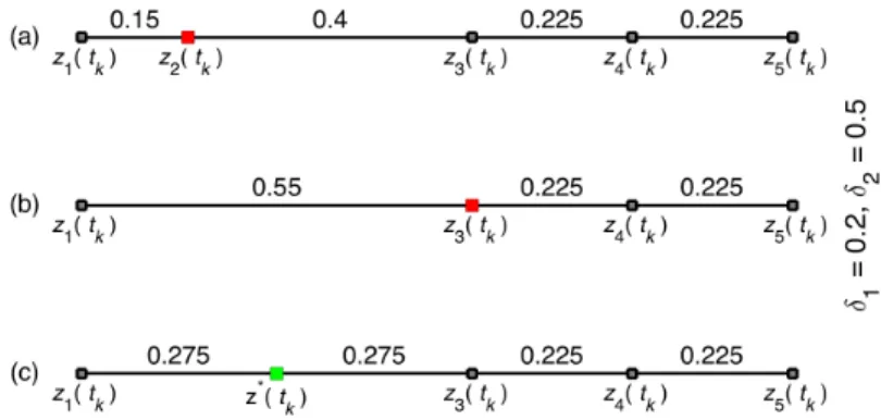
Figure 3.1: A simple illustration of the remeshing process withδ1= 0.2 andδ2 = 0.5: invalid mesh
(a)remove z2(tk) which violatesδ1 (b)and insert z∗(tk) not to violateδ2 (c)
old nodes. The number of nodes in a mesh may change after a remeshing. This has the implication
that the dimension of the state vector will not be constant in time. It is this feature that makes the
situation so different from standard DA and challenges us to create a new formulation.
The remeshing algorithm, withδ1/δ1 = 0.2/0.5, is illustrated in Figure 3.1, for the nodez1(tk)
at a particular timet=tk of the integration. The node z2(tk) has a distance of 0.15 fromz1(tk),
which is smaller than δ1: therefore,z2(tk) is removed (Figure 3.1(a)). The next node, nowz3(tk),
has distance 0.55 from z1(tk), which exceeds δ2 (Figure 3.1(b)): therefore a new node z∗(tk) is
introduced at the midpoint betweenz1(tk) and z3(tk) (Figure 3.1(c)).
Figure 3.2 shows and example of this remeshing procedure applied to a velocity-based adaptive
moving mesh using Burgers’ equation (see SECTION for details) as a physical model. We see how
the nodes, oriented along the horizontal axis, follow a moving front. In particular, the mesh, which
initially has 40 equally distributed nodes ends up having only 27 unevenly distributed nodes, as a
result of the remeshing procedure.
3.4 The model state and its evolution
Since both the physical value(s) representing the system and the mesh on which the PDE is
solved are evolved, we represent them both in the state vector The dimension of the state vector is
then 2N, where N is the number of mesh nodes:
x= (u1, u2, . . . , uN, z1, z2, . . . , zN)∈RN ×[0, L)N, (3.6)
where the zi are viewed as the mesh nodes and ui the values of the physical variableu atzi.
Figure 3.2: An illustration of adaptive moving mesh over time solving Burgers’ equation untilt= 1 on a domain z=(0,1]. In this example, the remeshing criteria are based on δ1 = 0.02 and δ2 = 0.05.
There are 40 initial adaptive moving mesh nodes and 27 at t= 1; these are shown in green and red, respectively.
advancement and remeshing. It will not be defined for every x ∈ RN ×[0, L)N. Indeed, the mesh nodes will need to satisfy (3.3). We therefore introduce VN ⊂[0, L)N by the condition that z= (z1, z2, . . . , zN)∈VN when (3.3) holds.
The model will be operating between observation times. If we sett=tk as an observation time
andt=tk+1 as the next time at which observations will be assimilated, the model will be integrated
with an adapting mesh, including Lagrangian evolution and possible multiple remeshings, fromtk
totk+1 If xk=x(tk), then we set this model evolution as a map
xk+1=M(xk). (3.7)
Note that if the original PDE (3.1) is nonautonomous, i.e.,f depends ont directly, thenMwill depend on kand we would write M=Mk. For convenience, we assumetk+1−tk is a multiple of the computational time step. Moreover, we begin and end each integration between observation
x∈RN ×V
N. Because of the tolerances ofδ1 and δ2 there are, however, constraints on N. Since
they are both divisors ofL, we can introduce N1 and N2 by
L=N1δ1 =N2δ2, (3.8)
and we can restrict N2 ≤N ≤N1. We can then viewMas acting on a larger space that puts all
of its possible domains together. To this end, we set XN =RN ×VN and, viewing eachXN as a distinct space, define
X=
N1
[
N=N2
XN, (3.9)
and cast M as a mapping from Xto itself, i.e., M:X→ X. We note again that N may change under this map, i.e.,N may be different for xk andxk+1. In other words, ifxk∈XNk, then we will
have for the next iterationxk+1 ∈XNk+1 with, in general, Nk6=Nk+1. 3.5 The Numerical Models
When testing the modified EnKF methodology described in the following chapters, we use two
numerical models and two types of synthetic observations: Eulerian and Lagrangian.
The first numerical model is the diffusive form of Burgers’ equation [1]
∂u ∂t +u
∂u ∂z =ν
∂2u
∂z2, z∈[0,1), t∈(0, T] (3.10)
with periodic boundary conditions u(0, t) =u(1, t). In our experiments, we set the viscosity ν =
0.08; the model (3.10) is hereafter referred to as BGM. Given that Burgers’ equation can be solved
analytically, it has been used in several DA studies (see, e.g. Cohn, 1993; [37], [38]).
As a second model, we use an implementation of the Kuramoto-Sivashinsky equation ([39])
∂u ∂t +ν
∂4u ∂z4 +
∂2u ∂z2 +u
∂u
∂z = 0, z∈[0,2π), t∈(0, T], (3.11)
which is also given periodic boundary conditions, and is referred to as KSM throughout this work.
Concentration waves, flame propagation, and free surface flows are among the problems for which this
equation is used. The higher order viscosity,ν, is chosen as 0.027 which makes (3.11) display chaotic
![Figure 3.2: An illustration of adaptive moving mesh over time solving Burgers’ equation until t = 1 on a domain z=(0,1]](https://thumb-us.123doks.com/thumbv2/123dok_us/8324919.2207246/35.918.309.603.119.443/figure-illustration-adaptive-moving-solving-burgers-equation-domain.webp)