ANALYSIS OF COMPLEX LIPID MIXTURES USING ULTRAHIGH-PRESSURE LIQUID CHROMATOGRAPHY-MASS SPECTROMETRY (UHPLC-MS)
Kelsey Elizabeth Miller
A dissertation submitted to the faculty at the University of North Carolina at Chapel Hill in partial fulfillment of the requirements for the degree of Doctor of Philosophy in the Department
of Chemistry.
Chapel Hill 2019
Approved by:
ii © 2019
iii ABSTRACT
Kelsey Elizabeth Miller: Analysis of Complex Lipid Mixtures Using Ultrahigh-Pressure Liquid Chromatography-Mass Spectrometry (UHPLC-MS)
(Under the direction of James W. Jorgenson)
This dissertation explores the method development of studying glycerophospholipids (GP), glycerolipids (GL), and sphingolipids (SP) using reverse-phase UHPLC-Mass Spectrometry (UHPLC-MS). Method development began with choosing between superficially porous particles (SPPs) and fully porous particles (FPPs) for the best stationary phase. Previous sonication column packing studies performed on C18 BEH FPPs were performed while packing SPP columns with the anticipation that the same effect of highly efficient columns could be achieved. When results could not be duplicated, C18 BEH FPPs were chosen for moving forward. Next, the solvent modifiers that provided the best ionization efficiency for lipid detection in positive and negative ion mode were explored. The combination of ammonium formate and formic acid provided the best results. In addition, other chromatographic and MS parameters were studied to understand what settings improved lipid detection. Preliminary testing on standards and a
iv
all these findings concludes with a final section that focuses on a non-targeted study that
compared the lipid profiles of inflammatory and anti-inflammatory macrophages and how nitric oxide influenced macrophage phenotype. Relative quantification and identification were
v
ACKNOWLEDGMENTS
There were many people who lent me a helping hand along the way and made my experience at UNC special. First, thank you to my advisor, JJ. Your intellect, patience, and humbleness are an inspiration, and I’m fortunate to have joined your lab before you retired. Thank you for your encouragement and guidance along every step of this journey. I’ll miss our discussions of everything ranging from science to current political events. You’ve taught me a lot about a variety of topics! In addition, thank you to my labmates. I appreciate the older graduate students, James Treadway, Stephanie Moore, Justin Godinho, and Dan Lunn for taking the time to teach me the inner workings of lab when I first joined. Thank you to Emily Imes for being a hard working undergraduate researcher and a fun presence in lab. Many thanks to Katie Simpson for being a wonderful labmate and confidant these past five years. Lab would have been very lonely without you. Plus, who would have been my treat buddy?
Thank you to Waters Corporation and Martin Gilar for their support of my research by sending consumables and giving advice. Thank you to Kathy Wood who has been such an encouraging person during my time at UNC. She truly believed in me and awarded me the Chancellor’s Doctoral Candidacy Award. Thank you to Brandie Ehrmann, CRiTCL’s Mass Spectrometry CORE Director, who is the reason this last chapter exists. When I was in desperate need of a mass spectrometer, so I could collect data for my last study she let me hook up my Frankenstein UHPLC to the MS core’s Orbitrap. She gave me as much time as I needed to run my analyses and helped me whenever a problem arose. She has such a generous soul.
vi
communicate to the Thermo Orbitrap, which is no small feat. James Taylor was also instrumental in this last chapter. James cultured all the macrophages for Chapter 5 and graciously taught me about his research. He also edited the last chapter and we talked at length about interpreting the results. I’m glad we were able to collaborate because it brought us closer together.
In addition to the people mentioned before, I’m so thankful to have made amazing and brilliant friends in graduate school. Rachael Kenney, I’ve enjoyed our many adventures together from the Bahamas to the West Coast and everything in between. Nicole Smiddy, I appreciate your equal enthusiasm about mermaids and Teen Mom. You two are always someone I can turn to for wisdom and support. Thank you for being considerate and kind.
Thank you to my parents, my sister (Courtney), brother-in-law (Daniel), boyfriend (Matt), and my dog (Raleigh). Your support has been invaluable during all these years of educational pursuit. Matt, I’m so glad we met; our relationship was the best result from grad school. I appreciate all the coding you wrote for my data in Chapter 5; you were a huge help. Thank you for always believing in me and being a calming force. You are my rock.
vii
TABLE OF CONTENTS
LIST OF TABLES ... xii
LIST OF FIGURES ... xiv
LIST OF ABBREVIATIONS ... xx
LIST OF SYMBOLS ... xxvi
CHAPTER 1 - Introduction to Lipidomics using Liquid Chromatography- Mass Spectrometry... 1
1.1 Introduction ... 1
1.2 Lipidomics ... 1
1.2.1 Lipid Classification and Nomenclature ... 2
1.2.2 Biological Role of Lipids ... 4
1.2.3 Analytical Challenges Inherent to Lipids ... 4
1.2.4 Analytical Techniques Used in Lipidomics ... 6
1.3 Chromatographic Theory ... 9
1.3.1 Separation Efficiency ... 9
1.3.2 van Deemter Theory ... 10
1.3.2.1 A-term ... 11
1.3.2.2 B-term ... 12
1.3.2.3 C-term ... 12
1.3.3 Ultra-High Pressure Liquid Chromatography-Mass Spectrometry UHPLC-MS) ... 12
viii
1.4 Scope of this Dissertation ... 14
1.5 Tables ... 16
1.6 Figures ... 17
REFERENCES ... 20
CHAPTER 2 – Selection of Stationary Phase Particles for Studying Lipids Using Reversed-Phase Chromatography ... 24
2.1 Introduction ... 24
2.1.1 Fully Porous Particles and Superficially Porous Particles ... 25
2.2 Column Packing and Efficiency ... 26
2.2.1 Previous Efforts with Packing BEH 1.9 μm Particles ... 26
2.2.2 Previous Efforts with Packing SPP ... 26
2.3 Parameters for Evaluating Packed Columns ... 26
2.3.1 Kinetic Plots ... 26
2.3.2 Flow Resistance and Permeability ... 28
2.3.3 Corrections for Interstitial Velocity ... 29
2.4 Materials and Methods ... 30
2.4.1 Chemicals and Materials ... 30
2.4.2 In-solution Optical Microscopy ... 31
2.4.3 Column Packing ... 31
2.4.4 Column Characterization ... 33
2.5 Results and Discussion ... 34
2.5.1 Effect of Solvent on Halo Peptide Particle Aggregation ... 34
2.5.2 Effect of Slurry Concentration on Column Performance ... 34
ix
2.6 Conclusions ... 38
2.7 Tables ... 39
2.8 Figures ... 46
REFERENCES ... 64
CHAPTER 3 – Method Development for Analyses of Lipids Using Reversed-phase Chromatography on Modified UHPLC-MS System ... 67
3.1 Introduction ... 67
3.2 Role of RPLC in Lipidomics ... 67
3.3 Phospholipids and Glycerolipids ... 68
3.4 Current State of Resolving Lipid Isomers ... 70
3.5 Materials and Methods ... 70
3.5.1 Chemicals and Materials ... 70
3.5.2 Sample Preparation for UHPLC-MS Analysis ... 71
3.5.3 Chromatographic and Mass Spectrometric Conditions ... 73
3.6 Results and Discussion ... 74
3.6.1 Optimal Mobile Phase Modifiers for Positive and Negative Ion Mode ... 74
3.6.2 Effect of Column Heater Temperature on Lipid Separation ... 76
3.6.3 Effect of MS Ion Source Temperature on Ionization Efficiency ... 77
3.6.4 Extraction of Lipids from Egg Yolk Compared to Standard ... 78
3.6.5 Separation of Lipid Isomers ... 78
3.7 Conclusions ... 80
3.8 Tables ... 81
3.9 Figures ... 90
x
CHAPTER 4 – Optimization of Microcapillary Column Length and Inner Diameter for Lipidomics Investigated with Gradient Analysis
by Ultrahigh-Pressure Liquid Chromatography-Mass Spectrometry ... 104
4.1 Introduction ... 104
4.1.1 Peak Capacity Theory ... 104
4.1.2 Precedent for Gradient Analysis Studies in Proteomics and Metabolomics ... 105
4.2 Materials and Methods ... 106
4.2.1 Chemicals and Materials ... 106
4.2.2 Preparation of UHPLC Capillary Columns ... 107
4.2.3 van Deemter Characterization of Columns ... 108
4.2.4 Sample Preparation for UHPLC-MS Analysis ... 108
4.2.5 Chromatographic and Mass Spectrometric Conditions ... 109
4.2.6 Peak Capacity Characterization ... 110
4.3 Results and Discussion ... 110
4.3.1 van Deemter Characterization of Columns ... 110
4.3.2 Gradient Analysis by UHPLC-MS ... 111
4.3.3 Comparison of Column Efficiency and Peak Capacity ... 112
4.4 Conclusions ... 113
4.5 Tables ... 115
4.6 Figures ... 119
REFERENCES ... 124
CHAPTER 5 – Nontargeted Phospholipid Profiling of Macrophage Phenotypes Influenced by Nitric Oxide Using Ultrahigh-Pressure Liquid Chromatography-Mass Spectrometry ... 126
xi
5.1.1 Implantable Biosensors ... 126
5.1.2 Macrophages ... 127
5.1.3 Nitric Oxide ... 128
5.1.4 Lipid Profiling Macrophage Phenotypes ... 129
5.2 Materials and Methods ... 131
5.2.1 Chemicals and Materials ... 131
5.2.2 Synthesis and Characterization of DETA/NO ... 132
5.2.3 Cell Culture and Treatment of DEX, LPS, and DETA/NO ... 133
5.2.4 Sample Preparation for UHPLC-MS Analysis ... 133
5.2.5 Chromatographic and Mass Spectrometric Conditions ... 134
5.2.6 Data Processing and Statistical Analysis of Phospholipid Profiles ... 135
5.3 Results and Discussion ... 136
5.3.1 Comparison of M(-) to M1 and M2 Macrophages... 136
5.3.2 Effect of M1 Treated with DETA/NO at Low and High Concentrations... 138
5.3.3 Effect of M2 Treated with DETA/NO at Low and High Concentrations... 140
5.4 Conclusions ... 142
5.5 Figures ... 143
REFERENCES ... 152
APPENDIX 5.1 LIST OF LIPIDS IDENTIFIED IN M-/M1/M2 COMPARISON ... 156
APPENDIX 5.2 LIST OF LIPIDS IDENTIFIED IN M1 AND NO COMPARISON ... 159
xii
LIST OF TABLES
Table 1.1. Classification of Lipids adapted from Liu, et al.8 ... 16 Table 2.1. Physical properties of BEH and Halo particles. ... 39 Table 2.2. Summary data of the efficiency of each column packed with
1.9 μm Waters BEH C18 particles in acetone. ... 40
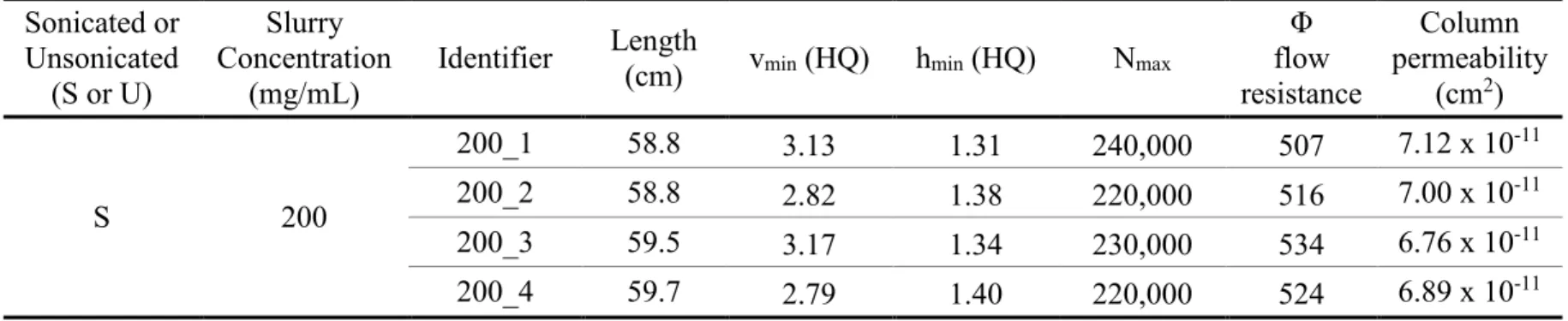
Table 2.3. Summary data of the efficiency of each column packed with
2.7 μm Halo particles in acetone at various slurry concentrations. ... 41 Table 2.4. Summary data of the efficiency of each column packed with
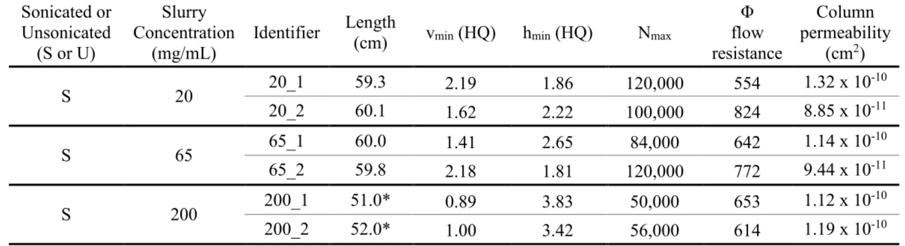
2.7 μm Halo particles in methanol at various slurry concentrations. ... 42 Table 2.5. Reduced van Deemter terms for each column packed in
acetone (BEH). ... 43 Table 2.6. Reduced van Deemter terms for each column packed in
acetone (Halo). ... 44 Table 2.7. Reduced van Deemter terms for each column packed in
methanol (Halo). ... 45 Table 3.1. Detection of different subclasses of phospholipids and
glycerolipids in positive and negative ion mode. An “X” means that
subclass can be detected in that ion mode. ... 81 Table 3.2. Ratios of signal intensity of each lipid compound detected
in positive ion mode in various mobile phase modifier conditions. The sample was a mixture of standards L-α-LysoPC and L-α-PC. Modifiers included 10 mM ammonium formate (AmF) + 0.1% formic
acid (FA), 0.1% formic acid, and 10 mM ammonium formate. ... 82 Table 3.3. Ratios of signal intensity of each lipid compound detected in
positive ion mode in various mobile phase modifier conditions. The sample was lipids extracted from chicken egg yolk. Modifiers included 10 mM ammonium formate (AmF) + 0.1% formic acid (FA),
0.1% formic acid, and 10 mM ammonium formate. ... 83 Table 3.4. Ratios of signal intensity of each lipid compound detected
in negative ion mode in various mobile phase modifier conditions. The sample was a mixture of standards L-α-LysoPC, L-α-PC, SM, L-α-PE, and L-α-PS. Modifiers included 10 mM ammonium formate (AmF) + 0.1% formic acid (FA), 10 mM ammonium acetate
(AmA) + 0.1% formic acid, and 10 mM ammonium acetate + 0.1%
xiii
Table 3.5. pH of mobile phase A and B with the modifiers used for positive ion mode. Modifiers included 10 mM ammonium formate (AmF) + 0.1% formic acid (FA), 0.1% formic acid,
and 10 mM ammonium formate. ... 85 Table 3.6. pH of mobile phase A and B with the modifiers used
for negative ion mode. Modifiers included 10 mM ammonium formate (AmF) + 0.1% formic acid (FA), 10 mM ammonium acetate (AmA) + 0.1% formic acid, and 10 mM ammonium
acetate + 0.1% acetic acid (AA). ... 86 Table 3.7. Combination of pressures and temperatures used to
achieve about 300 nL/min flow rate. ... 87 Table 3.8. Estimated lysoPC and PC identifications from
L-α-LysoPC and L-α-PC standards. ... 88 Table 3.9. Estimated PC identifications from lipids extracted
from chicken egg yolk. ... 89 Table 4.1. Peak capacity of each column at 2%, 4%, 8%, and
16% gradient rates... 115 Table 4.2. Reduced van Deemter terms for each column.
Test analyte is HQ in all cases. ... 116 Table 4.3. Peak capacity of each column at 2%, 4%, 8%,
and 16% gradient rates. ... 117 Table 4.4. Resolution of PC (Z 18:1/18:1) and PC (18:0/18:2) at
xiv
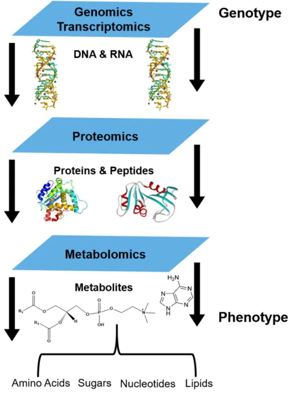
LIST OF FIGURES Figure 1.1 The omics platforms of a biological system adapted
from Courant, et al.3 ... 17 Figure 1.2 Example lipid PC18:0/18:1 (9Z) and its different types of
isomers. Changes are highlighted in red. A) sn position. B) Double bond
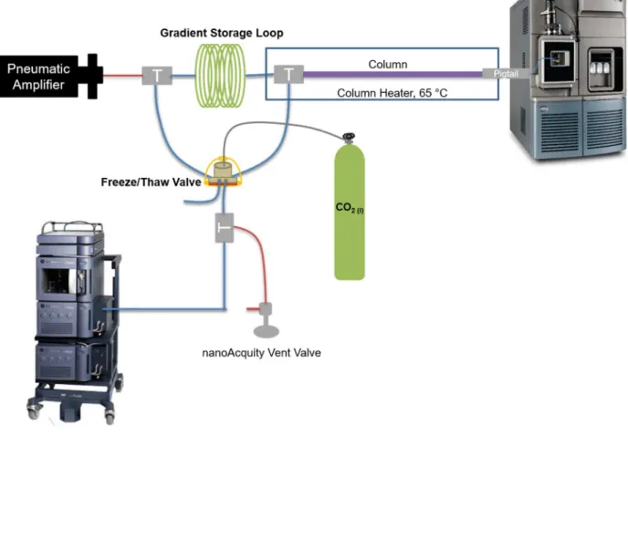
position. C) R/S chirality. D) cis/trans. ... 18 Figure 1.3 Schematic of the gradient UHPLC-MS system. Adapted
with permission from the dissertation of S. Moore.48 ... 19
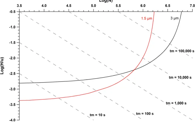
Figure 2.1 Example theoretical Poppe plots of 3 μm and 1.5 μm particles. Plots are constructed assuming pressure, ΔP = 1000 bar; viscosity,
η = 1 cP; interparticle porosity, εinterparticle = 0.49; analyte diffusion
coefficient, Dm = 6.14 x 10⁻⁶ cm2/s; reduced van Deemter coefficients
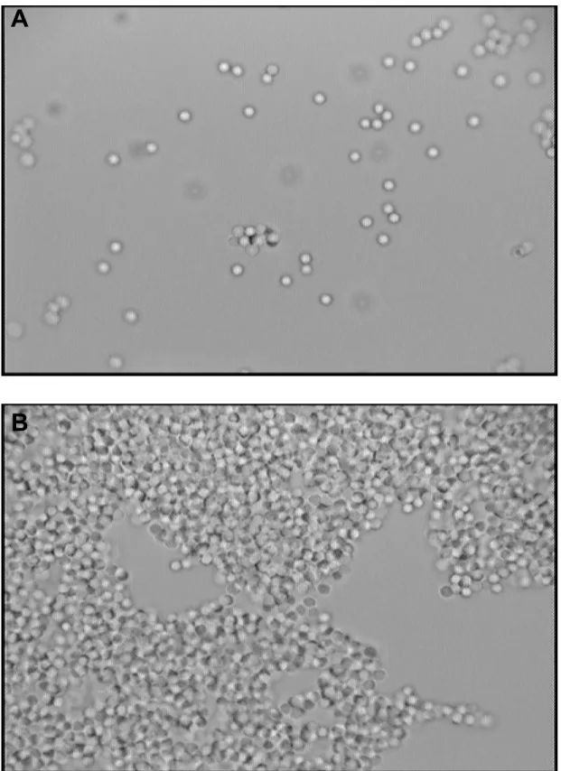
of a = 1.0, b = 1.0, and c = 0.1. ... 46 Figure 2.2 Images of 2.7 um Halo particles in acetone at varying
concentrations captured by in-solution microscopy. A) 3 mg/mL.
B) 25 mg/mL. ... 47 Figure 2.3 Images of 2.7 um Halo particles in methanol at varying
concentrations captured by in-solution microscopy. A) 3 mg/mL.
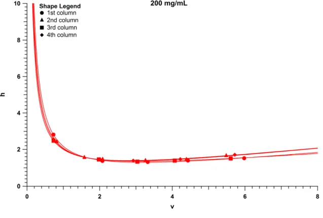
B) 25 mg/mL. ... 48 Figure 2.4 van Deemter curves of 60 cm 1.9 μm BEH capillary
columns packed at 200 mg/mL depicted in red. Test analyte is
Hydroquinone. ... 49 Figure 2.5 van Deemter curves of 60 cm 2.7 μm Halo capillary
columns packed in acetone at various slurry concentrations depicted
in black. Test analyte is Hydroquinone... 50 Figure 2.6 van Deemter curves of 60 cm* 2.7 μm Halo capillary
columns packed in methanol at various slurry concentrations depicted
in blue. Test analyte is Hydroquinone. ... 51 Figure 2.7 Comparison of van Deemter curves of BEH and Halo
capillary columns packed at 200 mg/mL and sonicated. BEH columns are red, Halo columns packed with acetone are black, and Halo columns
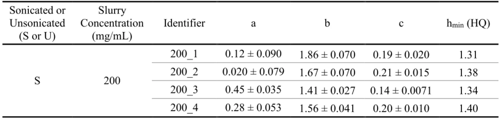
packed with methanol are blue. Test analyte is Hydroquinone. ... 52 Figure 2.8 Reduced minimum plate height (hmin) of each BEH column
packed in acetone at a slurry concentration of 200 mg/mL. Test analytes include A) Hydroquinone. B) Resorcinol. C) Catechol.
xv
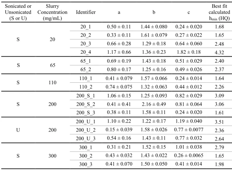
Figure 2.9 Reduced minimum plate height (hmin) of each Halo column
packed in acetone at various slurry concentrations. Test analytes include
A) Hydroquinone. B) Resorcinol. C) Catechol. D) 4-methyl catechol. ... 54 Figure 2.10 Reduced minimum plate height (hmin) of each Halo column
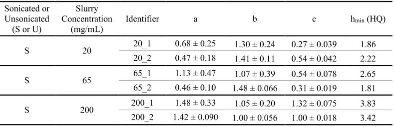
packed in methanol at various slurry concentrations. Test analytes include
A) Hydroquinone. B) Resorcinol. C) Catechol. D) 4-methyl catechol. ... 55 Figure 2.11 Flow resistance profiles for each BEH column packed in
acetone at 200 mg/mL slurry concentration illustrated in red. Theoretical flow resistance is displayed as a grey line. Corrections
for interstitial velocity were performed for each column. ... 56 Figure 2.12 Flow resistance profiles for each Halo column packed in
acetone at various slurry concentrations illustrated in black. Theoretical flow resistance is displayed as a light blue line. Corrections for
interstitial velocity were performed for each column. A) 20 mg/mL. B) 65 mg/mL. C) 110 mg/mL. D) 200 mg/mL sonicated.
E) 200 mg/mL unsonicated. F) 300 mg/mL... 57 Figure 2.13 Flow resistance profiles for each Halo column packed
in methanol at various slurry concentrations illustrated in blue. Theoretical flow resistance is displayed as a light blue line.
Corrections for interstitial velocity were performed for each column.
A) 20 mg/mL. B) 65 mg/mL. C) 200 mg/mL. ... 58 Figure 2.14 Averaged flow resistance profile for each BEH column
packed in acetone and each Halo column packed in acetone and methanol at 200 mg/mL slurry concentration sonicated. Experimental BEH flow resistance is red while experimental Halo in acetone is black and
experimental Halo in methanol is blue. Theoretical BEH flow resistance is displayed as a grey line and theoretical Halo flow resistance is illustrated as light blue. Corrections for interstitial velocity were performed for
each column. ... 59 Figure 2.15 Poppe plots of BEH capillary columns packed in acetone
at various slurry concentrations depicted in red. Theoretical Poppe plot of a BEH column is depicted as grey. Plots are constructed assuming pressure, ΔP = 1000 bar; viscosity, η = 1 cP; interparticle porosity, εinterparticle = 0.49; analyte diffusion coefficient, Dm = 6.14 x 10⁻⁶ cm2/s.
Theoretical Poppe plot uses reduced van Deemter coefficients of a = 1.0, b = 1.0, and c = 0.1. Experimental Poppe plots use reduced
van Deemter coefficients specific to that column given in Table 2.5. ... 60 Figure 2.16 Poppe plots of Halo capillary columns packed in acetone
xvi
assuming pressure, ΔP = 1000 bar; viscosity, η = 1 cP; interparticle porosity, εinterparticle = 0.39; analyte diffusion coefficient,
Dm = 6.14 x 10⁻⁶ cm2/s. Theoretical Poppe plot uses reduced van
Deemter coefficients of a = 1.0, b = 1.0, and c = 0.1. Experimental Poppe plots use reduced van Deemter coefficients specific to that
column given in Table 2.6. ... 61 Figure 2.17 Poppe plots of Halo capillary columns packed in
methanol at various slurry concentrations depicted in blue. Theoretical Poppe plot of a Halo column is depicted as light blue. Plots are
constructed assuming pressure, ΔP = 1000 bar; viscosity, η = 1 cP; interparticle porosity, εinterparticle = 0.39; analyte diffusion coefficient,
Dm = 6.14 x 10⁻⁶ cm2/s. Theoretical Poppe plot uses reduced van
Deemter coefficients of a = 1.0, b = 1.0, and c = 0.1. Experimental Poppe plots use reduced van Deemter coefficients specific to that
column given in Table 2.7. ... 62 Figure 2.18 Comparison of Poppe plots of BEH and Halo capillary
columns packed at 200 mg/mL and sonicated. BEH columns are red, Halo columns packed with acetone are black, and Halo columns packed with methanol are blue. Theoretical BEH Poppe plot is grey and theoretical Halo plot is light blue. Plots are constructed assuming pressure, ΔP = 1000 bar; viscosity, η = 1 cP; interparticle porosity, εinterparticle = 0.49 (BEH) and εinterparticle = 0.39 (Halo); analyte
diffusion coefficient, Dm = 6.14 x 10⁻⁶ cm2/s. Theoretical Poppe plot uses reduced van Deemter coefficients of a = 1.0, b = 1.0, and c = 0.1. Experimental Poppe plots use reduced van Deemter
coefficients specific to that column given in Tables 2.5-2.7. ... 63 Figure 3.1 General structure of glycerophospholipid and its subclasses. ... 90 Figure 3.2 Comparison of standards L-α-LysoPC and L-α-PC detected
in positive ion mode using different modifiers. From top to bottom chromatogram, 10 mM ammonium formate + 0.1% formic acid, 0.1% formic acid, and 10 mM ammonium formate. Numbered peaks are listed in Table 3.2. Peaks are as follows: 1) LysoPC (496.35 m/z), 2) LysoPC (524.38 m/z), 3) PC (758.59 m/z), 4) PC (810.62 m/z),
5) PC (760.56 m/z), 6) PC (786.61 m/z), 7) PC (788.62 m/z). ... 91 Figure 3.3 Comparison of lipids extracted from chicken egg yolk
detected in positive ion mode using different modifiers. From top to bottom chromatogram, 10 mM ammonium formate + 0.1% formic acid, 0.1% formic acid, and 10 mM ammonium formate. Numbered peaks are listed in Table 3.3. Peaks are as follows: 1) PC (806.56 m/z), 2) PC (782.54 m/z), 3) PC (758.52 m/z), 4) PC (808.56 m/z),
xvii
8) DG (601.52 m/z), 9) PC (788.60 m/z), 10) DG (603.54 m/z),
11) TG (874.78 m/z), 12) TG (876.82 m/z). ... 92 Figure 3.4 Comparison of standards L-α-LysoPC, L-α-PC, SM, L-α-PE,
and L-α-PS detected in negative ion mode using different modifiers. From top to bottom chromatogram, 10 mM ammonium
formate + 0.1% formic acid, 10 mM ammonium acetate + 0.1% formic acid, and 10 mM ammonium acetate + 0.1% acetic acid. Numbered peaks are listed in Table 3.4. Peaks are as follows: 1) LysoPC (480.30 m/z), 2) LysoPC (508.32 m/z),
3) LysoPC (681.31 m/z), 4) PS (780.50 m/z), 5) PS (782.50 m/z), 6) SM (747.54 m/z), 7) PC (802.54 m/z), 8) PE (714.51 m/z), 9) PC (804.55 m/z), 10) PC (830.57 m/z), 11) PE (716.51 m/z),
12) PE (742.54 m/z), 13) PC (832.58 m/z), 14) PE (744.54 m/z). ... 93 Figure 3.5 Comparison of L-α-LysoPC and L-α-PC standards analyzed
at various pressure and temperature combinations. The combination 60 °C, 25 kpsi was used as the control. Numbered peaks are listed in Table 3.2. Peaks are as follows: 1) LysoPC (496.35 m/z),
2) LysoPC (524.38 m/z), 3) PC (758.59 m/z), 4) PC (810.62 m/z),
5) PC (760.56 m/z), 6) PC (786.61 m/z), 7) PC (788.62 m/z). ... 94 Figure 3.6 Comparison of signal intensities of TG (54:3) and
TG (54:0) at various nanoESI source temperatures. ... 95 Figure 3.7 Comparison between a separation of A) L-α-PC standards,
a zoomed in chromatogram that does not show lysoPCs that eluted earlier, and B) lipids extracted from chicken egg yolk. Peaks are listed
in Table 3.8 and 3.9, respectively. ... 96 Figure 3.8 Attempt at resolving isomers PC (14:0/18:0) and
PC (18:0/14:0) on 60 cm in-house packed column. ... 97 Figure 3.9 Attempt at resolving isomers PC (16:0/18:1) and
PC (18:1/16:0) on 60 cm in-house packed column. ... 98 Figure 3.10 Attempt at resolving isomers PC (18:0/18:1) and
PC (18:1/18:0) on 60 cm in-house packed column. ... 99 Figure 3.11 Separation of PC (36:2) isomers using A) 25 cm
commercial column and B) 60 cm in-house packed column. ... 100 Figure 4.1 Selected van Deemter curves of columns 15_75_2,
30_75_3, 60_75_3, and 30_100_1. ... 119 Figure 4.2 Seven lipid standards were separated with a 2% gradient
rate on a 15.3 cm x 75 μm id column at 6.5 kpsi (black),
xviii
id column at 32 kpsi (red). Base peak (BPI) chromatograms of each
column are shown. ... 120 Figure 4.3 Peak capacity was calculated for each column at four gradient
rates (2%, 4%, 8%, and 16%). Three columns (circle, triangle, and square) were analyzed for each set of columns, which included 15 cm x 75 μm id columns (black), 30 cm x 75 μm id columns (blue), 60 cm x 75 μm id
columns (red), and 30 cm x 100 μm id columns (light blue). ... 121 Figure 4.4 Peak capacity is plotted against the square root of N. Three
columns (circle, triangle, and square) were analyzed for each set of columns, which included 15 cm x 75 μm id columns (black), 30 cm x 75 μm id columns (blue), 60 cm x 75 μm id columns (red), and 30 cm x 100 μm id columns (light blue). The linear trend calculated does not include 30 cm x 100 um id columns. A) 2% gradient.
B) 4% gradient. C) 8% gradient. D) 16% gradient. ... 122 Figure 4.5 Resolution of each lipid pair is plotted against the square
root of the reciprocal of each gradient rate. Three columns (circle, triangle, and square) were analyzed for each set of columns, which included 15 cm x 75 μm id columns (black), 30 cm x 75 μm id columns (blue), 60 cm x 75 μm id columns (red), and 30 cm x 100 μm id columns (light blue). A) PC (14:0/14:0) and (16:1/16:1). B) PC (Z 18:1/18:1) and (18:0/18:2). C) PC (18:0/18:2) and (E 18:1/18:1). D) PC (Z 18:1/18:1)
and (E 18:1/18:1). E) TG (18:1/18:1/18:1) and PC (18:0/18:0/18:0). ... 123 Figure 5.1 Variable importance in projection (VIP) plot of 25 lipids
(VIP scores Top 25) from unstimulated macrophage (M(-)) vs LPS
(M1) vs DEX (M2) comparison. ... 143 Figure 5.2 Heat map and dendrogram of 25 lipids (VIP scores Top 25)
from unstimulated macrophage (M(-)) vs LPS (M1) vs DEX (M2)
comparison. ... 144 Figure 5.3 Log2(fold change) heat map of 25 lipids
(VIP scores Top 25) from unstimulated macrophage (M(-)) vs
LPS (M1) vs DEX (M2) comparison. ... 145 Figure 5.4 Variable importance in projection (VIP) plot of 25 lipids
(VIP scores Top 25) from LPS (M1) vs LPS + non-NO releasing donor (5 μg/mL and 500 μg/mL) vs LPS + NO releasing donor
(5 μg/mL and 500 μg/mL) comparison. ... 146 Figure 5.5 Heat map and dendrogram of 25 lipids (VIP scores Top 25)
from LPS (M1) vs LPS + non-NO releasing donor (5 μg/mL and 500 μg/mL) vs LPS + NO releasing donor
xix Figure 5.6 Log2(fold change) heat map of 25 lipids
(VIP scores Top 25) from LPS (M1) vs LPS + non-NO releasing donor (5 μg/mL and 500 μg/mL) vs LPS + NO releasing donor
(5 μg/mL and 500 μg/mL) comparison. ... 148 Figure 5.7 Variable importance in projection (VIP) plot of 25
lipids (VIP scores Top 25) from DEX (M2) vs DEX + non-NO releasing donor (5 μg/mL and 500 μg/mL) vs DEX + NO releasing
donor (5 μg/mL and 500 μg/mL) comparison. ... 149 Figure 5.8 Heat map and dendrogram of 25 lipids
(VIP scores Top 25) from DEX (M2) vs DEX + non-NO releasing donor (5 μg/mL and 500 μg/mL) vs DEX + NO releasing donor
(5 μg/mL and 500 μg/mL) comparison. ... 150 Figure 5.9 Log2(fold change) heat map of 25 lipids
(VIP scores Top 25) from DEX (M2) vs DEX + non-NO releasing donor (5 μg/mL and 500 μg/mL) vs DEX + NO releasing donor
xx
LIST OF ABBREVIATIONS 2D-LC – Two-dimensional Liquid Chromatography
4MC – 4-methylcatechol AA – Acetic Acid
AA – Arachidonic Acid (ω-6, 20:4) AA – L-ascorbic acid
ACN – Acetonitrile Adrenic Acid (ω-6, 22:4)
ALA – α-linolenic acid (ω-3, 18:3) AmA – Ammonium Acetate AmF – Ammonium Formate BEH – Bridged-ethyl Hybrid BPI – Base Peak Intensity CAT – Catechol
CCL15 – Chemokine CC Ligand 15 CCL18 – Chemokine CC Ligand 18 CCL20 – Chemokine CC Ligand 20 CD86 – Cluster of Differentiation 86 CE – Collision Energy
Cer – Ceramide
CGM – Continuous Glucose Monitoring DB – Double Bond
xxi DCM – Dichloromethane
DETA – Diethylenetriamine DEX – Dexamethasone DG – Diacylglycerols
DGLA – Dihomo-γ-linolenic Acid (ω-6, 20:3) DHA – Docosahexaenoic Acid (ω-3, 22:6) DMEM – Dulbecco’s Modified Eagle Medium DPA – Docosapentaenoic Acid (ω-3, 22:5) ECN – Equivalent Carbon Number
EDA – Eicosadienoic Acid (ω-6, 20:2)
ELISA – Enzyme-Linked Immunosorbent Assay EPA – Eicosapentaenoic Acid (ω-3, 20:5)
ESI – Electrospray Ionization
ETE – Eicosatrienoic Acid (ω-3, 20:3), FA – Fatty Acyls
FA – Formic Acid
FBR – Foreign Body Response FPP – Fully Porous Particles GL – Glycerolipids
GP – Glycerophospholipids HCl -- Hydrochloric acid
xxii HQ – Hydroquinone
HRMS – High-resolution Mass Spectrometer i.d. – inner diameter
IL-27Rα – Interleukin-27 Receptor alpha IL-3 – Interleukin-3
IL-4 – Interleukin-4 IL-β – Interleukin-beta
iNOS – Inducible Nitric Oxide Synthase IPA – Isopropanol
LA – Linoleic Acid (ω-6, 18:2) LC – Liquid Chromatography
LIPID MAPS – LIPID Metabolites and Pathways Strategy LMSD – LIPID MAPS Structure Database
LPS – Lipopolysaccharide lysoPA – lysophosphatidic Acid lysoPC – lysophosphatidylcholine lysoPE – lysophosphatidylethanolamine lysoPG – lysophosphatidylglycerol lysoPI – lysophosphatidylinositol lysoPS – lysophosphatidylserine
L-α-LysoPC – L-α-Lysophosphatidylcholine L-α-PC – L-α-Phosphatidylcholine
xxiii L-α-PS – L-α-Phosphatidylserine
M(-) – Unstimulated Macrophage m/z – Mass-to-charge ratio
M1 – Pro-inflammatory Macrophage M2 – Anti-inflammatory Macrophage MeOH – Methanol
MG – Monoacylglycerol MS – Mass Spectrometry
MS/MS – Tandem Mass Spectrometry MSn – Sequential Mass Spectrometry
nanoESI – nanolectrospray ionization NLS – Neutral Loss Scanning
NMR – Nuclear Magnetic Resonance NO – Nitric Oxide
NOA – Nitric Oxide Analyzer o.d. – outer diameter
PA – Phosphatidic Acid
PBS – Phosphate Buffered Saline PC – Phosphatidylcholines
xxiv PIS – Precursor Ion Scanning
PK – Polyketides PL – Phospholipid PR – Prenol lipids PS – Phosphatidylserine
PUFA – Polyunsaturated Fatty Acid Q-Orbitrap – Quadrupole-Orbitrap QQQ – Triple Quadrupole
QTOF – Quadrupole-time-of-flight RES – Resorcinol
RF – Radio Frequency
RPLC – Reversed-phase Liquid Chromatography rpm – revolutions per minute
SEM – Scanning Electron Microscope SL – Saccharolipids
SL – Sphingolipids SP – Sphingolipids
SPP – Superficially Porous Particles SRM – Selected Reaction Monitoring ST – Sterol lipids
xxv TLC – Thin Layer Chromatography
TNF-α – Tumor Necrosis Factor-alpha
xxvi
LIST OF SYMBOLS %Δ/cv – % change per column volume
+ve – Positive ion mode a – reduced A-term
A-term – Eddy Diffusion b – reduced B-term
B-term – Longitudinal Diffusion c – reduced C-term
Cm – Mass transfer in the interparticle mobile phase
Cs – Mass transfer in the stationary phase
Csm – Mass transfer in the stagnant intraparticle mobile phase
C-term – Mass Transfer
DM – Analyte diffusion coefficient
dp – Particle size
H – Plate Height
h – reduced plate height
H/u – Plate time
K – Column permeability L – Column Length
N – Plate Number or Plate Count nc – Peak capacity
tg – Gradient time
xxvii tR – retention time
u – Linear Velocity
ui – Interstitial velocity
umeasured – Measured linear velocity
v – reduced velocity
-ve – Negative ion mode w – Peak width
γ – Obstruction factor ΔP – Pressure drop
ε – Interparticle volume of the mobile phase εinterparticle – Interparticle porosity
εintraparticle – Intraparticle porosity
εT – Total porosity
η – Viscosity
λ – Quality of the packed column bed σL – Spatial Variance
σt – temporal variance
Φ – Flow resistance
1
CHAPTER 1 - Introduction to Lipidomics using Liquid Chromatography-Mass Spectrometry
1.1 Introduction
Lipids are key components to sustaining life, as they contribute to membrane structure, provide energy storage, and participate in cell signaling. Despite their role as a building block for life, research concerning these molecules had not been widely explored until the early 2000s.1,2 Over the past two decades, the field of lipidomics has uncovered important functions and
pathways of lipids, which can be used to identify normal and diseased states. Given the extensive variability and multitude of these molecules, an analytical method is needed that provides
quantitative and qualitative data in a high throughput manner while maintaining high resolution. For these reasons, ultrahigh-pressure liquid chromatography—mass spectrometry (UHPLC-MS) has the potential to become the premier technique for separation of complex lipid mixtures and will be the focus of this dissertation.
1.2 Lipidomics
The omic studies used to characterize biological systems are genomics, transcriptomics, proteomics, and metabolomics.3 While genomics, transcriptomics, and proteomics reveal information about the flow of gene expression, metabolomics is the most downstream omic platform that can show changes in phenotype and function (refer to Figure 1.1). Since
2
as the comprehensive analysis of all low molecular weight compounds, usually less than 1500 Da, in a sample. Metabolites include lipids, sugars, nucleotides, and amino acids, among many other things. The subset of metabolomics that concentrates on the study of lipids is known as lipidomics, which aims to quantitatively or qualitatively characterize the lipidome of an organism.5 In 2003, the LIPID Metabolites and Pathways Strategy (MAPS) Lipidomics
Consortium was created to start several initiatives that would better develop the budding field of lipidomics and serve the international lipid research community.6 These initiatives included providing resources such as access to lipid nomenclature, databases, protocols, and standards, and establishing research cores that studied lipidomes.
1.2.1 Lipid Classification and Nomenclature
One LIPID MAPS initiative included creating the International Lipid Classification and Nomenclature Committee, which redefined lipids and developed standardized nomenclature.The outdated definition characterized lipids as soluble in organic solvents and insoluble in water.7
3
glycerolipids (GL), glycerophospholipids (GP), sphingolipids (SP), sterol lipids (ST), prenol lipids (PR), saccharolipids (SL), and polyketides (PK).
Since there are many structural components that describe a lipid, it is important to discuss the shorthand notation that will be used in this dissertation, which is fully outlined in “Shorthand notation for lipid structures derived from mass spectrometry” and based on LIPID MAPS
terminology.11 Glycerolipids, glycerophosphoslipids, and sphingolipids will be mentioned in this dissertation, so the following descriptions of shorthand notation that apply to these classes will be described. When stating a lipid, the lipid subclass abbreviation is followed by the total
number of fatty acyl (FA) carbon atoms and the total number of double bonds (DB) separated by a colon. For example, PC 34:1 describes a phosphatidyl choline (a subclass of GPs) that has 34 carbon atoms and one DB. When the FA chains connected to a glycerol backbone are known, they are notated with “_” when the sn-positions of the FA chains are unknown or with “/” when the sn-positions are known. PC 16:0_18:1 indicates that the sn-position of FA chains 16:0 and 18:1 are unknown. PC 16:0/18:1 indicates that 16:0 is in sn-1 position while 18:1 is in sn-2 position. GLs may have up to three FA chains, so the order would follow as sn-1, sn-2, sn-3 positions. In addition, subclasses can be prefaced with “lyso” when there is only one FA chain, and a missing FA chain can be notated as 0:0 (e.g. lysophosphatidylcholine (LPC) 16:0/0:0). Double bond configuration can be either trans/cis and are designated as E/Z. Double bond positions can be counted from the -COOH end or the -CH3 end of a FA chain. If counted from
the -COOH end, the double bond is notated with Δ. If counted from the -CH3 end, the double
4 1.2.2 Biological Role of Lipids
The diversity in lipid structure allows these molecules to serve numerous biological functions: provide the foundation for cellular membranes, act as a mechanism for energy storage, and cell signaling. The membrane is the most abundant cellular structure in all living matter, and the majority of eukaryotic membrane lipids are glycerophospholipids, sphingolipids, and
sterols.12 The self-assembled lipid bilayer is composed of two thin molecular sheets that construct the foundation of all biological membranes, as well as act as a permeable, protective barrier that compartmentalizes cells.13 For long term energy storage, triacylglycerols are
commonly used and are stored in muscle and adipose tissue cells.14 Finally, researchers have begun unraveling lipids’ role in cellular signaling. Membrane lipids can form precursors for second messengers and then activate intracellular processes.15 Some examples of signaling lipids include eicosanoids, phosphoinositides, sphingolipids and fatty acids. 16 These signaling lipids control cellular processes such as cell proliferation, apoptosis, metabolism and migration. As a result, any imbalance in the lipid signaling network can contribute to disease. Some examples of lipids’ contributions to disease include diabetes,17,18 heart disease,18,19 and Alzheimer’s
Disease.20,21 Given lipids’ role in disease progression, lipid profiling is a common technique to monitor changes between a healthy and a diseased host in the hopes that a biomarker can be discovered.
1.2.3 Analytical Challenges Inherent to Lipids
5
The number of lipid species found in biological systems has been estimated to be on the order of hundreds of thousands.22 This estimate is based on the fact that lipid structures can be arranged in many different ways. The lipid structure can vary in the FA chain length, the number of double bonds, the double bond position, and the cis/trans configuration of double bonds. As of May 2019, LIPID MAPS Structure Database (LMSD) contains 43,402 unique lipid structures for biologically relevant lipids from mammals, plants, bacteria, fungi, algae, and marine organism. Phospholipid species alone are estimated to contain 9,600 lipids and only about 8,000 of those compounds are cited in LMSD.7
Besides the sheer number of lipids that can exist in a sample, another challenge is the number of isomers that can exist at one molecular mass. The different types of isomerisms include sn isomerism, double bond position isomerism, R/S isomerism, and cis/trans isomerism. To illustrate this point, Figure 1.2 shows how PC 18:0/18:1 (9Z) with an exact mass of 787.609 m/z could be four other isomers with the same fatty acid chains and backbone. In Figure 1.2, the
6 1.2.4 Analytical Techniques Used in Lipidomics
Several analytical techniques are used in lipidomics research, such as separation technologies, spectroscopy, and mass spectrometry (MS). The classical technique for lipid analysis is thin layer chromatography (TLC) because this method is inexpensive and fast.5 However, TLC is limited for lipid identification and quantitation. Another commonly used fast technique is nuclear magnetic resonance (NMR). NMR can be used for quantitation over a wide dynamic range, but can suffer from low sensitivity. Two common analytical capabilities
employed in lipidomics research that offer better sensitivity and selectivity include shotgun techniques, like direct infusion mass spectrometry, and separation methods, like gas or liquid chromatography.4,23 While direct infusion mass spectrometry offers high throughput, the analysis
can suffer from matrix effects and ion suppression. In addition, without a separation technique beforehand, the distinction of isobars and isomers becomes a challenge. The use of front-end separation before the mass spectrometer decreases sample complexity, increases sensitivity, and adds additional qualitative information. As opposed to directly infusing lipid mixtures, the benefit of online separation is that lipids with low ionization efficiency can be separated from lipids with high ionization efficiency, which expands the potential of identifying other species.24 As a result, analyzing complex lipid mixtures or low abundant lipid species with a separation method in tandem with a mass spectrometer is preferred over direct infusion.
7
charge accumulation at the liquid surface at the tip of capillary. Then this charged liquid breaks into smaller and smaller droplets to form highly charged droplets. Finally, once the droplets become small enough, the electric field on their surface becomes large enough to desorb ions from the surface. The gas-phase ions enter the vacuum region of the interface that leads to the MS. In nanoelectrospray, smaller flow rates are used (<1000 nL/min), which allows for smaller sampling and low sample consumption.27 In addition, ionization efficiency, ion transmission, and sensitivity are improved. Furthermore, ESI is a soft ionization technique that produces minimal fragmentation, which allows for easier detection of molecules in a complex biological mixture.7
In lipidomics research, tandem mass spectrometry (MS/MS) is often used because it is advantageous for gathering structural details and subsequent characterization since different lipid classes and fatty acid chains typically have distinct fragment patterns characteristic to them. With each tandem spectrometer, different kinds of data acquisition modes can be utilized, such as MS/MS, MSE, and MSn.
The MS/MS scan modes include selected reaction monitoring (SRM), neutral loss (NLS), precursor ion (PIS), and product ion scanning. In SRM, the first and second mass analyzers monitor the selected precursor and product ions. In NLS, the first and second mass analyzer scan simultaneously, but with a constant mass offset chosen. In PIS, the first mass analyzer scans across a mass range and the second mass analyzer monitors a chosen product ion. In product ion scanning, a precursor ion is chosen for the first mass analyzer and the second mass analyzer scans all the fragments that are produced.
Unlike MS/MS, MSE is an unbiased acquisition mode. An MSE acquisition alternates between low-energy collision-induced dissociation and high-energy collision-induced
8
mass data, respectively.25,28 As opposed to other tandem MS acquisition modes, in one analytical run the analyzer obtains a full-scan accurate mass fragment, precursor ion and neutral loss information.29 In addition, no information is lost because no masses were preselected and the
analyzer can revisit the data in case any molecule was overlooked.
Unlike MS/MS and MSE, sequential mass spectrometry (MSn) functions allow product
ions to be isolated and trapped for multiple cycles of fragmentation. The notation ‘n’ represents the number of times the isolation-fragmentation-measurement cycle has been performed. This scan mode is useful for gleaning more fragmentation data, which can help with further structural elucidation.
Mass analyzers typically used in lipidomics include triple quadrupoles (QQQ),
quadrupole-time-of-flight (QTOF), and quadrupole-Orbitrap (Q-Orbitrap). Triple quadrupoles are often used for quantitative or shotgun methods and allow for all MS/MS scan modes to be used. MS/MS is suitable when surveying for specific lipid classes, so QQQ are used typically for targeted analyses and as such, offer high selectivity and sensitivity. However, QQQ suffer from low mass accuracy and cannot perform MSn scans.
High-resolution mass spectrometers (HRMS) include QTOF and Q-Orbitrap. QTOF analyzers have high scan rate and can acquire full product ion spectra quickly.5 In terms of acquisition, some MS/MS scan modes or MSE can be employed, but MSn cannot be performed.
MSE is beneficial for lipidomics due to the increased productivity and efficiency of data
collection. In addition, MSE is useful when analyzing an unknown lipid mixture or searching for
9
rates, especially the more scans that are performed. The research discussed in this dissertation uses a Waters Xevo QTOF and a Thermo Scientific Q Exactive HF-X Hybrid Quadrupole-Orbitrap.
1.3 Chromatographic Theory
Chromatography involves an analyte’s partitioning between two immiscible phases, the mobile phase and the stationary phase.31 Analytes in a mixture separate from one another due to each analyte’s different affinity for the mobile and stationary phase. Analytes with a higher affinity for the stationary phase will elute later than analytes with a lower affinity, and thus will have a longer retention time (tR). This dissertation concerns liquid chromatography (LC), in
which the mobile phase is liquid and the stationary phase is made of solid bonded particles. In order to understand the quality of columns packed and analyzed, an overview of
chromatographic terminology is given below. 1.3.1 Separation Efficiency
Column efficiency measures the quality of the separation and determines the resolution of a separation. It can be exemplified by the column’s plate number (N) and takes into account peak dispersion.32 Plate count is a dimensionless parameter that can be described by its relationship with retention time (tR) and temporal variance (σt2) or with column length (L) and spatial
variance (σL2):
= = (1-1)
The number of plates in a column can be used to calculate plate height (H), also known as the height equivalent to a theoretical plate (HETP):33
10
The variance of the peak (σL2) increases linearly with distance (L) that it has traveled. In
other words, an analyte injected onto the inlet of the column will begin as a narrow band, but this band will broaden as the analyte migrates through the column. The van Deemter theory describes the contributions to the band broadening process in more depth.
1.3.2 van Deemter Theory
The column plate height can be elaborated further by the van Deemter equation, which relates the theoretical plate height to linear velocity (u) and three broadening terms:34
= + + (1-3)
The A-term represents eddy diffusion or the analyte’s random flow path through a packed column bed, the B-term accounts for longitudinal diffusion in the mobile phase, and the C-term explains the resistance to mass transfer in the mobile phases. Each broadening term can be expanded further and the van Deemter equation can be written as:
= + + (1-4)
Where H is described by quality of the packed bed (λ), particle size of column packing material (dp), obstruction factor (γ), mass-transfer coefficient (χ), and analyte diffusion coefficient (DM).
By minimizing H, plate count will increase, and thus, column efficiency will improve. One way to reduce H is to pack columns with smaller particles since plate height is proportional to particle diameter. However, in order to compare columns packed and operated under varying conditions, velocity and plate height must be reduced to v and h, respectively. Reduced
11
≡ (1-5)
ℎ ≡ (1-6)
From here, the van Deemter can be written in reduced terms:
ℎ = ! + "
#+ $ (1-7)
1.3.2.1 A-term
Eddy dispersion occurs in a packed bed because the flow path is tortuous and provides multiple paths of varying lengths for the analyte to travel. In addition, the velocity of some paths differs from other paths.33 For instance, the particles packed along the wall are not as densely packed as the particles in the center of the column. As a result, a higher velocity exists alongside the wall than in the center of the column. This leads to analyte migrating close to the wall to elute earlier than analyte flowing through the center of the bed. The A-term reflects the quality of a packed column and can be expressed as:
= % (1-8)
The λi factor represents the quality (uniformity) of the packed bed with values ranging
from 0.5 to 2. Obtaining a homogeneous bed structure while column packing is important. A smaller λi factor signifies a higher level of structural uniformity across the packed bed, and thus,
12 1.3.2.2 B-term
Longitudinal diffusion describes molecular diffusion in the axial direction.33 If a solute were to sit in the column bed unperturbed, then over time the solute’s band will spread and diffuse into the surrounding areas. The B term can be expressed as:
& = 2( (1-9)
The obstruction factor (γ) accounts for the obstruction that the solute faces in terms of free movement. Generally, the B term has little effect in LC, especially if higher mobile phase
velocities are used. 1.3.2.3 C-term
The phenomena of mass transfer resistance first involve an analyte traveling from the mobile phase to the surface of the stationary phase particle. Then the analyte is transported through the stagnant mobile phase in the particle’s pores. Finally, the analyte interacts with the stationary phase before then traveling back into the flowing mobile phase. The resistance to mass transfer can be divided into mass transfer in the interparticle mobile phase (Cm), mass transfer in
the stationary phase (Cs), and mass transfer in the stagnant intraparticle mobile phase (Csm). An
in-depth explanation of the C-term is beyond the scope of this dissertation.
1.3.3 Ultra-High Pressure Liquid Chromatography-Mass Spectrometry UHPLC-MS) Ultra-high-pressure liquid chromatography (UHPLC) is a method of liquid
chromatography that is an improvement upon high-pressure liquid chromatography (HPLC) in terms of column efficiency.37 In HPLC, typically columns with 2.0-4.6 mm i.d. packed with 3-5
13
resolution in comparison to HPLC. In addition, UHPLC offers faster flow rates and shortened analysis times.
However, packing smaller i.d. columns with smaller particles causes increased
backpressure. The pressure drop across a column packed with particles can be described as39:
∆* = +, (1-10)
As seen from Eq. 1-10, the pressure drop across the column is inversely proportional to the square of the particle diameter (dp) and directly proportional to flow resistance (Φ), viscosity
(η), column length (L), and velocity (u). Consequently, UHPLC is characterized by the use of high pressures that range from 6,000 to 100,000 psi.35
1.3.4 The Role of UHPLC-MS in Lipidomics
To address the challenges of lipidomics research (isobars, isomers, low abundant species, a wide range of solute polarities), a high throughput, highly sensitive, and high resolving power technique is needed. Capillary UHPLC meets these requirements because it is one of the most sensitive, efficient, and high resolution techniques available.40 As mentioned before, to increase resolving power, either column length must increase and/or particle size must decrease.
However, changing these parameters comes at the expense of increased backpressure. Furthermore, the viscous solvents typically needed in lipidomics studies increase the backpressure as well.41 The use of higher temperatures can reduce this issue by decreasing solvent viscosity, but too high of temperatures risk degrading silica-based stationary phases.42–44 Another solution is to increase operation pressure, but most commercial UHPLC systems can provide pressures only up to 20,000 psi.45
14
order to reach very high pressures, the commercial instrument, a Waters nanoacquity UPLC, has been modified to operate with extra features. When preparing for an analysis, the Waters UPLC loads the gradient and sample in reverse onto the capillary gradient storage loop. To start the analysis, liquid CO2 freezes the fluid in the capillary tubing in the freeze/thaw valve, so the flow
is redirected toward the column and MS. The pneumatic amplifier pushes the gradient and sample from the gradient storage loop through the column and into the MS for detection. Also featured on the modified UHPLC system are highly efficient in-house packed columns with sub-2 μm particles that produce about 500,000 theoretical plates per meter and achieve minimum reduced plate height values approaching 1.47 The high resolving power and increased peak capacity of these columns introduce the potential to better separate complex mixtures. These higher efficiency columns could be advantageous in a field like lipidomics where a diverse range of species exists.
There is much potential for discovery of lipid species and further elucidation of disease states and understanding how biological systems function. By combining the power of the modified UHPLC and HRMS, we gain an analytical method that provides high resolution, improved separation, accurate mass measurement, and structural identification information useful for investigating lipidomes.25 This specialized combination can be applied to analyzing complex lipid samples and performing targeted and non-targeted analyses.
1.4 Scope of this Dissertation
15
optimizing LC and MS conditions by testing ionization efficiency of lipids under different mobile phase conditions and mass spectrometer parameters. Proof of concept work demonstrates how resolution of lipids improves on the UHPLC MS system. Chapter 4 reviews a
16 1.5 Tables
17 1.6 Figures
18
19
20
REFERENCES
(1) Lagarde, M.; Géloën, A.; Record, M.; Vance, D.; Spener, F. Lipidomics Is Emerging. Biochim. Biophys. Acta 2003, 1634 (3), 61.
(2) Han, X.; Gross, R. W. Global Analyses of Cellular Lipidomes Directly from Crude Extracts of Biological Samples by ESI Mass Spectrometry. J. Lipid Res. 2003, 44 (6), 1071–1079.
(3) Courant, F.; Antignac, J. P.; Dervilly-Pinel, G.; Le Bizec, B. Basics of Mass Spectrometry Based Metabolomics. Proteomics 2014, 14 (21–22), 2369–2388.
(4) Kuehnbaum, N. L.; Britz-McKibbin, P. New Advances in Separation Science for Metabolomics Resolving. Chem. Rev. 2013, 113, 2437–2468.
(5) Köfeler, H. C.; Fauland, A.; Rechberger, G. N.; Trötzmüller, M. Mass Spectrometry Based Lipidomics: An Overview of Technological Platforms. Metabolites 2012, 2 (1), 19– 38.
(6) Schmelzer, K.; Fahy, E.; Subramaniam, S.; Dennis, E. A. The Lipid Maps Initiative in Lipidomics. Methods Enzymol. 2007, 432 (07), 171–183.
(7) Brügger, B. Lipidomics: Analysis of the Lipid Composition of Cells and Subcellular Organelles by Electrospray Ionization Mass Spectrometry. Annu. Rev. Biochem. 2014, 83 (1), 79–98.
(8) Wenk, M. R. The Emerging Field of Lipidomics. Nat. Rev. Drug Discov. 2005, 4 (7), 594–610.
(9) Fahy, E.; Subramaniam, S.; Brown, H. A.; Glass, C. K.; Merrill, A. H.; Murphy, R. C.; Raetz, C. R. H.; Russell, D. W.; Seyama, Y.; Shaw, W.; et al. A Comprehensive Classification System for Lipids. J. Lipid Res. 2005, 46 (5), 839–862.
(10) Li, M.; Yang, L.; Bai, Y.; Liu, H. Analytical Methods in Lipidomics and Their Applications. Anal. Chem. 2014, 86 (1), 161–175.
(11) Liebisch, G.; Vizcaíno, J. A.; Köfeler, H.; Trötzmüller, M.; Griffiths, W. J.; Schmitz, G.; Spener, F.; Wakelam, M. J. O. Shorthand Notation for Lipid Structures Derived from Mass Spectrometry. J. Lipid Res. 2013, 54 (6), 1523–1530.
(12) Simons, K.; Sampaio, J. Membrane Organization and Lipid Rafts. Cold Spring Harb. Perspect. Biol. 2011, 3 (10), 1–17.
21 Basis of Life; 2012.
(15) Fernandis, A. Z.; Wenk, M. R. Membrane Lipids as Signaling Molecules. Curr. Opin. Lipidol. 2007, 18 (2), 121–128.
(16) Wymann, M. P.; Schneiter, R. Lipid Signalling in Disease. Nat. Rev. Mol. Cell Biol. 2008, 9 (2), 162–176.
(17) Janikiewicz, J.; Hanzelka, K.; Kozinski, K.; Kolczynska, K.; Dobrzyn, A. Islet β-Cell Failure in Type 2 Diabetes - Within the Network of Toxic Lipids. Biochem. Biophys. Res. Commun. 2015, 460 (3), 491–496.
(18) Meikle, P. J.; Wong, G.; Barlow, C. K.; Weir, J. M.; Greeve, M. A.; MacIntosh, G. L.; Almasy, L.; Comuzzie, A. G.; Mahaney, M. C.; Kowalczyk, A.; et al. Plasma Lipid Profiling Shows Similar Associations with Prediabetes and Type 2 Diabetes. PLoS One 2013, 8 (9).
(19) Stegemann, C.; Drozdov, I.; Shalhoub, J.; Humphries, J.; Ladroue, C.; Didangelos, A.; Baumert, M.; Allen, M.; Davies, A. H.; Monaco, C.; et al. Comparative Lipidomics Profiling of Human Atherosclerotic Plaques. Circ. Cardiovasc. Genet. 2011, 4 (3), 232– 242.
(20) Han, X.; Rozen, S.; Boyle, S. H.; Hellegers, C.; Cheng, H.; Burke, J. R.; Welsh-Bohmer, K. A.; Doraiswamy, P. M.; Kaddurah-Daouk, R. Metabolomics in Early Alzheimer’s Disease: Identification of Altered Plasma Sphingolipidome Using Shotgun Lipidomics. PLoS One 2011, 6 (7), 1–13.
(21) Chan, R. B.; Oliveira, T. G.; Cortes, E. P.; Honig, L. S.; Duff, K. E.; Small, S. A.; Wenk, M. R.; Shui, G.; Di Paolo, G. Comparative Lipidomic Analysis of Mouse and Human Brain with Alzheimer Disease. J. Biol. Chem. 2012, 287 (4), 2678–2688.
(22) Pöhö, P.; Kivilompolo, M.; Calderon-Santiago, M.; Jäntti, S.; Wiedmer, S. K.; Hyötyläinen, T.; Poho, P.; Kivilompolo, M.; Calderon-Santiago, M.; Jantti, S.; et al. Chapter 9 Applications. In Chromatographic Methods in Metabolomics; 2013; pp 195– 227.
(23) Han, X.; Gross, R. W. Shotgun Lipidomics: Electrospray Ionization Mass Spectrometric Analysis and Quantitation of Cellular Lipidomes Directly from Crude Extracts of
Biological Samples. Mass Spectrom. Rev. 2005, 24 (3), 367–412.
(24) Taguchi, R.; Nishijima, M.; Shimizu, T. Basic Analytical Systems for Lipidomics by Mass Spectrometry in Japan. Methods Enzymol. 2007, 432, 185–211.
22
(26) Kebarle, P. Electrospray: From Ions in Solution to Ions in the Gas Phase, What We Know Now. Mass Spectrosc. Rev. 2009, 28, 35–49.
(27) Gibson, G. T. T.; Mugo, S. M.; Oleschuk, R. D. Nanoelectrospray Emitters: Trends and Perspective. Mass Spectrosc. Rev. 2009, 28 (6), 35–49.
(28) Zhao, Y. Y.; Cheng, X. L.; Vaziri, N. D.; Liu, S.; Lin, R. C. UPLC-Based Metabonomic Applications for Discovering Biomarkers of Diseases in Clinical Chemistry. Clin. Biochem. 2015, 47 (15), 16–26.
(29) Wrona, M.; Mauriala, T.; Bateman, K. P.; Mortishire-Smith, R. J.; O’Connor, D. “All-in-One” Analysis for Metabolite Identification Using Liquid Chromatography/Hybrid Quadrupole Time-of-Flight Mass Spectrometry with Collision Energy Switching. Rapid Commun. Mass Spectrom. 2005, 19 (18), 2597–2602.
(30) Lin, L.; Lin, H.; Zhang, M.; Dong, X.; Yin, X.; Qu, C.; Ni, J. Types, Principle, and
Characteristics of Tandem High-Resolution Mass Spectrometry and Its Applications. RSC Adv. 2015, 5 (130), 107623–107636.
(31) Jönsson, J. Å. Chromatographic Theory and Basic Principles; 1987. (32) Snyder, L. R.; Kirkland, J. J.; Dolan, J. W. Introduction to Modern Liquid
Chromatography; 2010.
(33) Neue, U. D. HPLC Columns, Theory, Technology, and Practice; 1998.
(34) Wren, S. A. C.; Tchelitcheff, P. Use of Ultra-Performance Liquid Chromatography in Pharmaceutical Development. J. Chromatogr. A 2006, 1119 (1–2), 140–146.
(35) Jorgenson, J. W. Capillary Liquid Chromatography at Ultrahigh Pressures. Annu. Rev. Anal. Chem. 2010, 3 (1), 129–150.
(36) Gritti, F.; Guiochon, G. Mass Transfer Kinetics, Band Broadening and Column Efficiency. J. Chromatogr. A 2012, 1221, 2–40.
(37) Dong, M. W.; Zhang, K. Ultra-High-Pressure Liquid Chromatography (UHPLC) in Method Development. TrAC - Trends Anal. Chem. 2014, 63, 21–30.
(38) Gumustas, M.; Kurbanoglu, S.; Uslu, B.; Ozkan, S. A. UPLC versus HPLC on Drug Analysis: Advantageous, Applications and Their Validation Parameters.
Chromatographia 2013, 76 (21–22), 1365–1427.
(39) Wu, N.; Clausen, A. M. Fundamental and Practical Aspects of Ultrahigh Pressure Liquid Chromatography for Fast Separations. J. Sep. Sci. 2007, 30 (8), 1167–1182.
23 6 (2), 443–458.
(41) Cajka, T.; Fiehn, O. Comprehensive Analysis of Lipids in Biological Systems by Liquid Chromatography-Mass Spectrometry. TrAC - Trends Anal. Chem. 2014, 61, 192–206. (42) Borges, E. M.; Volmer, D. A. Silica, Hybrid Silica, Hydride Silica and Non-Silica
Stationary Phases for Liquid Chromatography. Part II: Chemical and Thermal Stability. J. Chromatogr. Sci. 2015, 53 (7), 1107–1122.
(43) Greibrokk, T.; Andersen, T. High-Temperature Liquid Chromatography. J. Chromatogr. A 2003, 1000 (1–2), 743–755.
(44) Wenclawiak, B. W.; Giegold, S.; Teutenberg, T. High-Temperature Liquid Chromatography. Anal. Lett. 2008, 41 (7), 1097–1105.
(45) Fekete, S.; Kohler, I.; Rudaz, S.; Guillarme, D. Importance of Instrumentation for Fast Liquid Chromatography in Pharmaceutical Analysis. J. Pharm. Biomed. Anal. 2014, 87, 105–119.
(46) Grinias, K. M.; Godinho, J. M.; Franklin, E. G.; Stobaugh, J. T.; Jorgenson, J. W. Development of a 45 Kpsi Ultrahigh Pressure Liquid Chromatography Instrument for Gradient Separations of Peptides Using Long Microcapillary Columns and Sub-2 Μm Particles. J. Chromatogr. A 2016, 1469, 60–67.
(47) Godinho, J. M.; Reising, A. E.; Tallarek, U.; Jorgenson, J. W. Implementation of High Slurry Concentration and Sonication to Pack High-Efficiency, Meter-Long Capillary Ultrahigh Pressure Liquid Chromatography Columns. J. Chromatogr. A 2016, 1462, 165– 169.
24
CHAPTER 2 – Selection of Stationary Phase Particles for Studying Lipids Using Reversed-Phase Chromatography
2.1 Introduction
Separation efficiency is proportional to column length and plate height, therefore, long columns with small plate heights are ideal for maximizing separation efficiency (see Equation 1-2). For this reason, our lab has used one-meter long columns packed with 1.7 μm bridged-ethyl hybrid (BEH) fully porous particles (FPP) for separating complex biological mixtures.1–3 For
lipidomic analyses, the goal was to use one-meter long columns as well, but the backpressure was too high to use a column at this length due to the selection of mobile phases. Lipid analysis using reversed-phase chromatography commonly consists of water and isopropanol in the gradient system. These two more viscous solvents cause higher back pressure than the water-acetonitrile reversed-phase gradient normally used in a capillary LC system.
One solution to reducing back pressure is to use columns packed with superficially porous particles (SPP). Studies have shown that 2.7 μm SPP provide comparable or improved column efficiency to 1.7 μm BEH FPP.4–9 These studies were performed with standard bore columns, so we were interested to see if these kinds of results could translate to capillary
25
columns packed with 1.7 μm BEH FPP and columns packed with 2.7 μm Halo SPP, in order to select the best stationary phase for separating lipids without compromising resolution.
2.1.1 Fully Porous Particles and Superficially Porous Particles
Given the advent of UHPLC instrumentation, sub-2 μm fully porous particles have become widespread since the mid-2000s.10 Silica based fully porous particles are the most
popular, but cause large back pressure. Superficially porous particles, or core-shell particles, serve as an attractive alternative because the operating pressure is 2-2.5 times less.11 The
operating pressure is reduced significantly due to the presence of a solid core in the middle of the particle, which is surrounded by porous shell layer. This geometry results in more rapid
intraparticle mass transfer, so that larger diameter particles may be used and operating pressure is reduced. This sorbent has become more popular due to this significant advantage. In addition, these particles claim to have improved performance compared to FPP due to a decrease in A-term and C-A-term contributions. Although most research with these particles has been with standard bore columns, our lab has conducted research about packing these particles in capillary columns.12–14 Currently, lipid research conducted using core-shell capillary columns has not been
26 2.2 Column Packing and Efficiency
2.2.1 Previous Efforts with Packing BEH 1.9 μm Particles
Previous work from our lab demonstrated that column efficiency is dictated partially by the slurry concentration used when packing columns. A slurry concentration that is too low or too high will decrease the column efficiency. A study completed by Justin M. Godinho, et al., showed that ultrasonication while packing columns increases their performance.16 In this study, one-meter-long columns were packed with BEH silica particles at a slurry concentration of 200 mg/mL. These columns produced about 500,000 theoretical plates and achieved minimum reduced plate height values approaching 1, which is unprecedented. The addition of
ultrasonification while packing allowed for column packing using high slurry concentrations that previously resulted in poor column efficiency.
2.2.2 Previous Efforts with Packing SPP
While previous lab members have packed capillary columns with SPP, the element of sonification while packing has not been applied. Laura Blue packed 2.7 μm Halo particles and found a reduced plate height below 1.9.12 She worked on discovering tools that would predict
optimal packing conditions. For example, one tool called in-solution optical microscopy looks at how particles behave in different solvents at atmospheric pressure. She found that in-solution optical microscopy can predict whether a slurry solvent is suitable or not and found that aggregating solvents generated the most efficient columns.
2.3 Parameters for Evaluating Packed Columns 2.3.1 Kinetic Plots
27
particle sizes in consideration of specific pressures and other parameters, a researcher can determine which column is more suitable when a fast analysis time or a highly efficient separation is needed.17
Poppe plots are generally expressed as plate time (H/u) vs. the plate number (N), in which plate time is defined as the amount of time it takes to generate one theoretical plate. For example, Figure 2.1 illustrates a theoretical Poppe Plot that compares a column packed with 3 μm particles to a column packed with 1.5 μm particles. In the lower left portion of the plot, a smaller particle size of 1.5 μm would provide a smaller plate time and better separation efficiency at faster analysis times than a column packed with 3 μm particles. The horizontal asymptote represents the limitation in terms of speed and very short analysis time. The highest separation efficiency can be achieved only with the larger particle size at the cost of longer analyses, which is displayed in the upper right region of the Poppe plot. The vertical asymptote represents the limiting plate count at very long analyses. The point where the two curves intersect is when each column would provide the same separation efficiency with the same analysis time. The dotted lines intersecting the curves at various points represent different dead times (tm).
To help create a theoretical or experimental Poppe plot, the Kozeny-Carman equation can be used:18,19
% =
-. /
012, (04/) (2-1)
Pressure drop (ΔP), particle diameter (dp), interparticle volume of the mobile phase (ε),
and viscosity (η) are kept constant. By changing the column length (L), interstitial velocity (ui)
28
In order to create theoretical and experimental Poppe plots, Equations 1-5, 1-6, and 1-7 must be rearranged. The diffusion coefficient (DM) along with interstitial velocity and particle
diameter can be calculated to determine reduced velocity (v). Then reduced van Deemter coefficients (a, b, c) and reduced velocity can be used to calculate reduced plate height (h). Finally, plate height (H) can be calculated. When creating the Poppe plots, plate number (N) can be calculated by dividing column length by its respective plate height. Then the log of N and the log of plate height divided by linear velocity are taken and plotted.
Poppe plots comparing Halo particles to C18 BEH particles have been presented in the literature before. Wang, et. al completed a study that compared the performance of 2.1 mm id columns packed with Halo 2.7 μm C18 SPP to BEH 1.7 μm C18 FPP columns with Poppe plots.6
They found that Halo particles outperform BEH particles when operated beyond analysis times of 10 seconds. At analyses longer than 1,000 seconds, the plate count of Halo columns was two-fold higher than BEH columns.
2.3.2 Flow Resistance and Permeability
Monitoring pressure drop over a column can give insight into the packed bed structure. For example, flow resistance (Φ) is a dimensionless parameter defined as:20,21
Φ = -.
, (2-2)
The geometry of the particles (e.g. roughness, porosity, etc.) influences the flow
29
Another closely related parameter is the column permeability K (cm2), which indicates how easily fluid flows through the column and is defined as:23
7 = ,
-. (2-3)
The column bed permeability to solvent flow decreases with decreasing particle diameter and with wider particle size distributions.20 In addition, superficially porous particles would be
expected to have a higher permeability than similar sized fully porous particles.24,25 2.3.3 Corrections for Interstitial Velocity
Measured linear velocity (umeasured) is based on the time it takes for an unretained
compound to elute from a column:18
89:; <9 =
=
(2-4)
While using this velocity works well for non-porous particles, a more accurate velocity to use for porous particles is interstitial velocity (ui):
% = >?@ABC?D /E
/FG ?C @C FHI?
(2-5)
By knowing the total porosity (εT) and interparticle porosity (εinterparticle), the measured
linear velocity can be corrected to the interstitial velocity. Total column porosity can be further divided into interparticle porosity and intraparticle porosity:26
JK = J%L 9< :< %MN9+ J%L <: :< %MN9(1 − J%L 9< :< %MN9) (2-6)
εinterparticle is the porosity between particles while εintraparticle represents the porosity of the