Modeling and Control of Server Systems: Application to Database Systems

Modeling and Control of Server Systems:

Application to Database Systems

Luc Malrait, Nicolas Marchand and Sara Bouchenak

Abstract— Servers technology is a mean to support different Internet services and applications ranging from web servers, to email systems, streaming media services, enterprise servers, and database servers. However, the ad-hoc configuration of servers poses significant challenges to the performance and economical costs of applications. This paper precisely addresses this issue. Firstly, we present the design of a server model as a non-linear continuous-time model. A fluid flow approach allows us to partly free ourselves from accurate stochastic considerations. Secondly, a utility function for characterizing the impact of server configuration on performance and cost is presented. Thirdly, a utility-aware capacity planning algo-rithm is developed to efficiently control the configuration of servers. Model and control algorithm were implemented and applied to the standard PostgreSQL database server running the TPC-C warehouse application. The experiments show that the proposed method provides significant benefits for database servers management.

I. INTRODUCTION

A large variety of Internet services exists, ranging from web servers to e-mail servers [1], [2], [3], streaming media services [4], enterprise servers [5], [6], and database sys-tems [7], [8]. These services are usually based on the client-server architecture, where a client-server provides some online service (such as reading web pages, sending emails or buying the content of a shopping cart), and clients concurrently access that service.

In addition to this concurrent access, the workload of a server (i.e. the number of concurrent clients and the nature of their requests) may vary over time, from a light one to a heavy one and vice versa. For instance, an e-mail server is likely to face a heavier workload in the morning than in the rest of the day, since people usually consult their e-mails when arriving at work. In its extreme form, a heavy workload may induce server thrashing and service unavailability, with underlying economical costs. For instance, the downtime cost for companies in the Telecom and Financial companies is estimated at up to US$ 2.0 million/hour [9], [10], [11]. A classically used technique to prevent a server from thrashing when the workload increases is admission control [12]. It consists in fixing a limit for the maximum number of client allowed to concurrently access a server – known as the Multi-Programming Level (MPL) configuration parameter of a server.

L. Malrait is with NeCS research team, INRIA - Gipsa-lab, Grenoble, France,[email protected]

N. Marchand is with NeCS research team, CNRS - Gipsa-lab, Grenoble, France,[email protected]

S. Bouchenak is with SARDES research team, INRIA - University of Grenoble I, Grenoble, France,[email protected]

Obviously, servers’ MPL configuration and control has a direct impact on servers performance and quality-of-service (QoS). While the MPL is usually manually configured by human administrators in an ad-hoc way in real server sys-tems, some algorithms for adaptive adjustment of MPL were proposed [13]. However, they are restricted to a performance model with a parabola shape which is not the case of performance criteria such as client request latency and client request rejection rate [14]. Other work aiming at applying control theory to server systems appeared in the last decade. A first approach applies well-known linear control theory on servers modeled as SISO or MIMO black-boxes [15], [16]. However, due to the deep nonlinear behavior of real server systems, linear control theory is obviously insufficient for these systems [17]. Other approaches are based on nonlinear models derived from queuing theory [18], [19] with a theoreticalproposal [17], [20], [21]. These approaches are hardly applicable because the statistical properties of the connections and of the server need to be known.

In this paper, a nonlinear continuous-time model based on a fluid flow approach is proposed. To the author knowledge, this seems to be the first available with such a range of validity. In order to validate the model, it is validated with a real database server system and used for control purposes. The main scientific contributions of this paper are the following:

• Design and implementation of a nonlinear continuous

time modelof server systems in Section III,

• Design and implementation of a firstnonlinear control law for the capacity planning of server systems in Section IV,

• Experimental validation of the proposed model and

control law in a real system consisting of the Post-greSQL database server running the TPC-C warehouse application [7], [22] in Section V.

II. CONTEXT AND PRELIMINARY DEFINITIONS

Server systems such as database servers and web servers follow the client-server architecture where a client connects to a server which provides him some online service, e.g. on-line bookstore, e-banking, etc. Clients and servers are hosted on different computers connected through a communication network. Basically, a client remotely connects to the server, sends it a request, the server processes the request and builds a response that is returned to the client before the connection is closed. Multiple client requests may concurrently access the same server.

a) Server workload: is characterized, on one hand, by the number of client requests that try to concurrently access a server (i.e.workload amount), and on the other hand, by the nature of those requests (i.e.workload class), e.g. read-only requests or read-write requests. The former is denoted as _N while the latter is denoted as _C. Furthermore, server workload may vary over time. This corresponds to different client behaviors at different times. For instance, an e-mail service faces a higher workload in the morning than in the rest of the day.

b) Think time: of a client is the elapsed duration

between the reception of a reply and the sending of another connection request. It corresponds to the time spent by a client in reading a page and “thinking” before the next request. The think time depends on the server workload’s nature, and the average think time is denoted as_{LT T}.

c) Admission control: is a classical technique to prevent

a server from thrashing when the number of concurrent client requests grows [12]. It consists in fixing a limit for the maximum number of client requests allowed to concurrently access a server – the Multi-Programming Level (_{M P L}) con-figuration parameter of a server. Above this limit, incoming client requests are rejected. Thus, a client request arriving at a server either terminates successfully with a response to the client, or is rejected because of the server’s_{M P L}limit. Therefore, due to the MPL limit, among the _N clients that try to concurrently access a server, only _Ne clients really access the server (_Ne≤_{M P L}).

Servers’ _{M P L} value has a direct impact on the perfor-mance and quality-of-service (QoS) of servers. Here, several performance metrics may be considered [23], among which:

d) Server throughput: is defined as the the number of

served requests per second. It is denoted as_To. A high server throughput (or throughput, for short) is a desirable behavior which reflects the speed of the server. A high_{M P L}usually implies a high throughput when the server is not overloaded.

e) Client request latency: is defined as the time needed

by the server to process a request. It corresponds to the time duration between the instant when a client request arrives and the instant when the response is sent back. The average client request latency is denoted as_L. A low client request latency (or latency, for short) is a desirable behavior which reflects a reactive system. A low _{M P L} usually implies a low latency.

f) Client request rejection rate: is defined as the ratio

of requests rejected due to admission control compared to the total number of requests received by a server. It is denoted as_α. A low client request rejection rate (or rejection rate, for short) is a desirable behavior that reflects service availability. A high_{M P L}usually implies a low rejection rate.

g) SLA – Service Level Agreement –: is a contract

negotiated between clients and their service provider like a server system [14]. It specifies service level objectives (SLOs) for performance guarantied by the service, like the maximum latency _Lmax, the minimum throughput _Tomin and the maximum rejection rate _αmax to be guaranteed by the server.

III. SERVER MODEL

The choice of the control inputs, the system outputs and the state variable outputs is crucial for the design of a model. As the_{M P L}is a tunable parameter of a server and has a meaningful effect on its performance, it is natural to take it as control input of the system. We assume that the state of the system can be described by three variables: the current number of concurrent requests in the server_Ne, the throughput_Toand the rejection rate_α. The server workload amount N can be seen as an exogenous input. Obviously, the outputs will depend on the chosen SLOs.

A balance on _Nebetween_t and_t+_dt gives: Ne(t+dt) =Ne(t) +created connections

−closed connections According to the assumptions, the number of connections closed between_tet_dt+_tis_To(_t)·_dt. Let_Ti be the number of connection demands per second._Tiobviously depends on the load, but also on the state of the server. Indeed, since clients wait for a reply before making again a connection demand, shorter is the latency, higher is _Ti. It comes that the number of connections created between_t and_t+_dt is

(1−α(t))·Ti(N, t)·dt. Finally, it follows:

˙

Ne= (1−α(t))·Ti(N, t)−To(t) (1)

The next step will consist in writing Ti as a function of

N._Ti can be considered as the ratio between the number of clients and the average interarrival time of the requests. Since only the accepted connections are submitted to the server’s latency, the average interarrival time is (1−_α(_t))_L(_t) + LT T. Thus we get

Ti(N, t) =₍₁₋ N(t)

α(t))L(t) +LT T

Now we assume that:

1) The dynamics of _To and _α with respect to _N are a pure delay that corresponds to the average latency_L. 2) The average latency _L is much smaller than the

dy-namic of_Ne and than the load variations.

The first assumption states that for a given load, _To and α reach their steady state values when the first request is served. Instead of focusing on the statistical properties of the throughput, its average is considered here. In practice, the second assumption is natural since the average latency is very small w.r.t. the variations induced by connection changes. Under these assumptions, the dynamics of_To and_αcan be approximated by first order systems:

˙

To(t) =−

1

L(t)

To(t)−T¯o

˙

α(t) =− 1

L(t)(α(t)−α¯)

where_T¯_o and_α¯are the steady state values corresponding to a constant demand of connections.

The next step naturally consists in finding the expressions of_T¯_o and_α¯. In steady state, a balance on the served request number_Nogives:

No(t+dt) =No(t) +served requestduring dt Since the _Ne is the current number of concurrent requests and the average latency is _L, the number of served request during _dt will be dt_LNe. Then we get _N˙_o = Ne

L, that is

¯

To = N_Le which is an expression of Little’s law [24]. By

definition, α¯ is equal to 1−To

Ti if Ne =M P L, otherwise it is equal to zero. The problem is that the stochastic nature of the requests arrival may provoke a rejection even if the average _Ne measured is smaller than the _{M P L}. Thus we choose to write _α¯ = Ne

M P L ·

1−To

Ti

. It renders that the probability to reject a connection is higher when the average Neis close to the M P L. Therefore, it finally follows:

˙

To(t) =− 1

L(t)

To(t)−Ne(t)

L(t)

(2)

˙

α(t) =− 1 L(t)

α(t)− Ne(t) nmax(t)·

1−To(t)

Ti(t)

(3)

0 10 20 30 40 50 60 70 0

5 10 15 20 25

N_e

Latency (s)

Fig. 1. Latency as a function ofNe

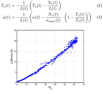
The last step is to express the latency as a function of the state and the inputs. The latency obviously depends on the load’s nature_C. Write requests are often longer to process than read-only requests and read-only requests may be more or less costly in cpu time. It depends also on _Ne because the requests that have to be processed at the same time share the cpu between them. This effect is amplified by the context switch mechanism that occurs during the processes preemption. Seeing the difficulty in designing an accurate knowledge model for the latency, we limit ourselves to the design of a behavior model. One can see on Figure 1 that a second degree polynomial in_Neis a good approximation of the latencyL. Thus:

L=a(C, t)Ne2+b(C, t)Ne+c(C, t) (4)

The parameter c is positive as it represents the zero-load latency.aandb are also positive since they model the cost in time of the requests.

Finally, the proposed server’s model is given by equa-tions (1) to (4). Its validation comes in section V and the

next section is dedicated to a first admission control strategy based on this server’s model.

IV. SERVER CONTROL

In the following, a first control law is proposed based on the server’s model given in the previous section. The control objective, that is the desired QoS, is here a maximum latency _Lmax to be guaranteed (cf. Section II). Besides this maximum latency, a minimum rejection rate has to be ensured. In that aim, a feedback control law is proposed to automatically adjust the _{M P L} in order to satisfy these control objectives.

One assumes that the whole state of the system (that is Ne,Toandα), the latencyLconsidered as the output of the

system as well as the number of connection demands per second _Ti can be measured in real time. On the contrary, N is considered as unknown and not measurable. All these assumptions are in accordance with the experimental context. Fig. 2 shows the framework of the study.

Server

System

Capacity

Monitor Planner

Clients

MP L N

Lmax

Fig. 2. Framework of the study

A first approach could consist in solving L(M P L, t) =Lmax. This solution implies that the

parameters _a, _b and _c in equation 4 of the model can be perfectly online identified, since the workload may change over time. Therefore, an another solution avoiding this identification of the model’s parameters was preferred. It is obtained by a simple input-output linearization approach. Its stability is straightforward to establish.

Let us consider that the dynamic of the load’s variations is much smaller than the average latency. It follows:

L(Ne) =aNe2+bNe+c

α(t) = ¯α To(t) = ¯To

Let us take the latency _L as output. It follows that _L˙ =

(2aNe+b) ˙Ne. From (1) and (3) one has

˙

L= (2aNe+b)

1− Ne

M P L Ti−T¯o

Therefore, taking

M P L= Ne

1 +γ L−Lmax

(Ti−T¯o)(2aNe+b)

will ensure that_L˙ =−_γ(_L−_Lmax)and therefore, as soon as_{γ >}0, the exponential convergence of_Lto its maximum Lmax corresponding to the desired QoS. Unfortunately, this

requires the knowledge of_aand_b. Therefore, it seems better to take:

M P L= Ne

1 +γL−Lmax

Ti−Ne y

(5)

whereγ>0 is some tuning parameter. It follows that with control (5), the time evolution of_Lis given by:

˙

L=−γ(2aNe+b) (L−Lmax)

and therefore again,_L will exponentially converge to_Lmax since2_aNe+_{b >}0.

V. EVALUATION

A. Experimental Setup

The experimental setup is composed of two computers, one for the database server and one for the clients emulator. The server runs on a PC 3 GHz with 2GB RAM, while the clients’ computer is a PC 2 GHz with 512MB RAM. Op-erating system is Linux Fedora 7 for both. PostGresql-8.2.6 was taken as database server [7]. To evaluate the server’s performance the TPC-C benchmark [22] was used, which emulates a warehouse application using five transaction types (with read and write requests). Both client and server are largely used in the computer science community.

B. Model Identification and Validation

The load of a server is strongly time-varying and the mechanisms used by the server to process the requests are dependent on this load. A write request will need a hard drive access, a read only request may already be in the hard drive cache and another one may be very costly for the cpu. The complexity of those mechanisms and the impredictability of the load urged us to design a very general model with fewer parameters as possible. In order to show the effectiveness of the server’s model, an off-line identification of the parameters is processed and then, on a different scenario, the real server and the model are compared. It implies that:

• we are able to measure the number of clients trying to interact with the server.

• the load’s nature will be the same for both identification and validation experiments.

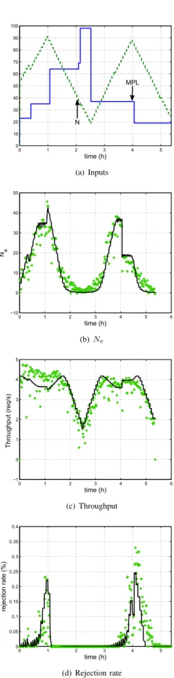
To identify the parameters_a,_band_ca nonlinear optimization algorithm was used with an experimental input-output data set. To obtain this data set, the maximum multiprogramming level of the server was increased from 3 to 100 with a workload of 100 clients. The cost function to minimize is the sum of the squares of the difference between the real latency and the estimate one. The _{LT T} parameter is given by the benchmark. The obtained parameters of the server are _a= 0_.0015, _b = 0_.2210, _c = 0_.0554 and_{LT T} = 12_s. Results are presented in 3(a), 3(b), 3(c) and 3(d). Figure 3(a) shows the scenario used in open loop according to the time in hours: the dashed line isN and the solid line is the MPL. Figures 3(b), 3(c) and 3(d) show respectively the evolution of _Ne,_To and _α according to the time for the real system (+) and for the model (solid line). The model renders well the behavior of the real system. We can observe a trashing

(a) Inputs

0 1 2 3 4 5 6 7

0 10 20 30 40 50 60 70 80

time (h)

Ne

(b)Ne

0 1 2 3 4 5 6 7

0 0.5 1 1.5 2 2.5 3 3.5 4 4.5

time (h)

Throughput (req/s)

(c) Throughput

0 1 2 3 4 5 6

0 0.1 0.2 0.3 0.4 0.5 0.6 0.7

time (h)

rejection rate (%)

(d) Rejection rate

Fig. 3. Evolution of the state and the inputs in open loop for the real system (+) and for the model (solid line).

0 1 2 3 4 5 0

10 20 30 40 50 60 70 80 90 100

time (h) MPL

N

(a) Inputs

0 1 2 3 4 5 6

−10 0 10 20 30 40 50

time (h)

Ne

(b)Ne

0 1 2 3 4 5 6

−1 0 1 2 3 4 5

time (h)

Throughput (req/s)

(c) Throughput

0 1 2 3 4 5

0 0.05 0.1 0.15 0.2 0.25 0.3 0.35 0.4

time (h)

rejection rate (%)

(d) Rejection rate

Fig. 4. Evolution of the state and the inputs in open loop for the real system and for the model.

phenomenon on these figures since_Tois decreasing whereas Ne is increasing. This effect could not be seen without an

overlinear term with respect to _Ne in equation (4). The floor we observe on _Ne and _To from the fourth hour of the experiment shows that not all the clients have a request in process at the same time. It is a direct impact of the think time.

We present on figures 4(a), 4(b), 4(c) and 4(d) experi-mental validations obtained by generating several random numbers of clients and random maximum MPLs. Figure 4(a) shows the scenario used in open loop according to the time in hours: the dashed line is N and the solid line is the MPL. This scenario is more dynamic than the previous one since sudden changes of the MPL appear. Figures 4(b), 4(c) and 4(d) respectively show the evolution of the MPL, the throughput and the rejection rate according to the time for the real system (+) and for the model (solid line). The model well describes the behavior of the system. The maximum prediction errors between the model and the real system is 21% for _Ne 13% for _To and 28% for the rejection rate. These errors can be explained by the growth of the database provided by the benchmark during an experiment. Indeed the database is 10 % bigger at the end of the experiment than at the beginning. Thus there are more and more hard drive requests, that slows down the system. Even if only one type of requests is used, the system is practically always evolving, and an online identification of the parameters is absolutely necessary to be able to render accurately the system behavior.

C. Control Evaluation

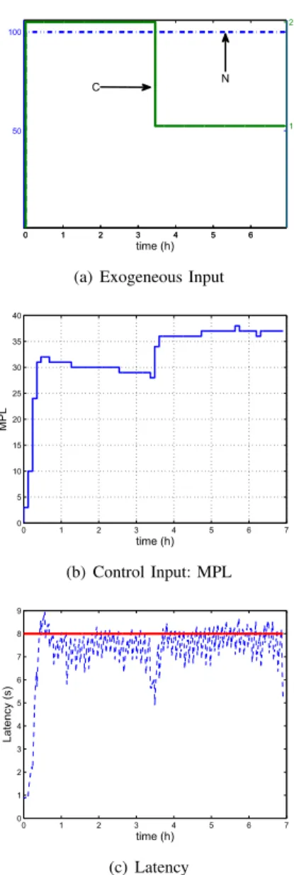
The main difficulty in implementing a controller for server capacity planner in a real system lies in the fact that the default MPL of the server is not dynamically tunable. For our experiments, we followed a proxy-based approach which uses a connection pool in front of the server to control the number of authorized connections in that pool. The number of authorized connections is updated every 6 minutes by the control input calculated with the online measurements. The maximum latency _Lmax was set to 8 seconds. The results presented in this section show the efficiency of the controllers designed in section IV. We see on Figure 5(a) the exogenous inputs of the system. The number of clients_N was fixed to 100. The workload class 1 is made of read-write requests and the class 2 of read-only requests. Figure 5(c) shows the latency according to the time. We see that it converges to 8 seconds, and that the rising time to 90% is approximatively half an hour. Fig 5(b) shows the MPL calculated with (5).

VI. CONCLUSION AND PERSPECTIVES

It clearly appears that server systems need a dynamical tuning to avoid trashing and to ensure service level ob-jectives. A general continuous time model of a server was presented here. It is able to render both dynamical and static behavior of a real one. Even if the model’s parameters have to be updated online to get an accurate approximation of the server’s behavior, we proposed a simple control law that allows to respect service level objectives that do not

0 1 2 3 4 5 6 50

100

time (h)

0 1 2 3 4 5 6

1 2

C N

(a) Exogeneous Input

0 1 2 3 4 5 6 7

0 5 10 15 20 25 30 35 40

time (h)

MPL

(b) Control Input: MPL

0 1 2 3 4 5 6 7

0 1 2 3 4 5 6 7 8 9

time (h)

Latency (s)

(c) Latency

Fig. 5. Evolution of the latency (dashed line) and the inputs forLmax= 8s

(solid line).

rely on this parameters. The example presented in section V only considers a latency constraint but one can imagine that several QoS constraints could be considered. For instance the rejection rate is an important QoS factor, because it is useless to ensure a small latency if nobody can connect to the server. In a future work, we will consider optimizing the MPL of a server so that several QoS constraints can be respected. Moreover, the application of server control on more complex systems distributed Internet services as in [25], [26] will be studied.

VII. ACNOWLEDGEMENTS

We would like to thank Jean Arnaud, Christophe Taton and Sylvain Durand for their technical help on the experimental environment and their feedback on previous versions of this work.

REFERENCES [1] Sendmail.org, 2007, http://www.sendmail.org/.

[2] M. T. E. server, 2007, http://technet.microsoft.com/en-us/exchange/. [3] W. Venema, The postfix home page, 2007, http://www.postfix.org/. [4] A. Inc., “QuickTime Streaming Server,” 2007,

http://www.apple.com/quicktime/streamingserver/. [5] A. Inc, 2007, http://www.amazon.com/.

[6] eBay Inc, 2007, http://www.ebay.com/. [7] P. G. D. Group, “Postgresql,” 2008. [8] Oracle, “Oracle,” 2008.

[9] I. Mountain, “The business case for disaster recovery planning: Cal-culating the cost of downtime,” 2001, iron Mountain.

[10] N. A. S. I. Inc., “The true cost of downtime,” 2008, http://www.nasi.com/downtime cost.php.

[11] J. Paransky, “Case studies for the cost of downtime,” 2008,

http://www.stacksafe.com/blog/case-studies-for-the-cost-of-downtime/04/02/2008/.

[12] J. Hyman, A. A. Lazar, and G. Pacifici, “Joint Scheduling and Ad-mission Control for ATS-based Switching Nodes,” inThe ACM Con-ference on Communications Architecture and Protocols (SIGCOMM ’92), Baltimore, MA, Aug. 1992.

[13] H.-U. Heiss and R. Wagner, “Adaptive load control in transaction pro-cessing systems,” inVLDB ’91: Proceedings of the 17th International Conference on Very Large Data Bases. San Francisco, CA, USA: Morgan Kaufmann Publishers Inc., 1991, pp. 47–54.

[14] J. Lee and R. Ben-Natan, Integrating Service Level Agreements. Wiley, 2002.

[15] S. Parekh, N. Gandhi, J. Hellerstein, D. Tilbury, T. Jayram, and J. Bigus, “Using control theory to achieve service level objectives in performance management,”Real-Time Syst., vol. 23, no. 1-2, pp. 127–141, 2002.

[16] Y. Diao, N. Gandhi, J. Hellerstein, S. Parekh, and D. Tilbury, “Using mimo feedback control to enforce policies for interrelated metrics with application to the apache web server,”Network Operations and Management Symposium, 2002. NOMS 2002. 2002 IEEE/IFIP, pp. 219–234, 2002.

[17] M. Kihl, A. Robertsson, and B. Wittenmark, “Analysis of admission control mechanisms using non-linear control theory,”Computers and Communication, 2003. (ISCC 2003). Proceedings. Eighth IEEE Inter-national Symposium on, pp. 1306–1311 vol.2, 30 June-3 July 2003. [18] D. Tipper and M. Sundareshan, “Numerical methods for modeling

computer networks under nonstationary conditions,”Selected Areas in Communications, IEEE Journal on, vol. 8, no. 9, pp. 1682–1695, Dec 1990.

[19] W.-P. Wang, D. Tipper, and S. Banerjee, “A simple approximation for modeling nonstationary queues,”INFOCOM ’96. Fifteenth Annual Joint Conference of the IEEE Computer Societies. Networking the Next Generation. Proceedings IEEE, vol. 1, pp. 255–262 vol.1, 24-28 Mar 1996.

[20] M. Kihl, A. Robertsson, and B. Wittenmark, “Performance modelling and control of server systems using non-linear control theory,” inIn 18th International Teletraffic Congress, Berlin, Germany, Sep. 2003. [21] A. Robertsson, B. Wittenmark, M. Kihl, and M. Andersson,

“Ad-mission control for web server systems - design and experimental evaluation,”Decision and Control, 2004. CDC. 43rd IEEE Conference on, vol. 1, pp. 531–536 Vol.1, 14-17 Dec. 2004.

[22] TPC, “Tpc transaction processing performance council,” 2008. [23] D. A. Menasc, D. Barbara, and R. Dodge, “Preserving QoS of

E-Commerce Sites Through Self-Tuning: A Performance Model Ap-proach,” in ACM Conference on Electronic Commerce (EC’01), Tampa, FL, Oct. 2001.

[24] J. D. C. Little, “A proof for the queueing formula L=λW,”Operation Research, vol. 9, pp. 383–387, 1961.

[25] S. Bouchenak, N. de Palma, D. Hagimont, and C. Taton, “Autonomic Management of Clustered Applications,” inIEEE International Con-ference on Cluster Computing (Cluster 2006), Barcelona, Spain, Sep. 2006.

[26] C. Taton, S. Bouchenak, N. de Palma, and D. Hagimont, “Self-Optimization of Internet Services with Dynamic Resource Provision-ing,” Tech. Rep. RR-6575, 2008.