Deteriorating Items Inventory Model Having Exponential Declining Demand with Inflation and Learning Effect under Credit Financing Policy

e-ISSN: 2278-5728, p-ISSN: 2319-765X. Volume 16, Issue 6 Ser. I (Nov. – Dec. 2020), PP 14-22 www.iosrjournals.org

Deteriorating Items Inventory Model Having Exponential Declining

Demand with Inflation and Learning Effect under Credit Financing

Policy

Jyoti,

Geetanjali Sharma

1_{Research Scholar,} 2_{Associate Professor}

Department of Mathematics and Statistics, Banasthali Vidyapith, Rajasthan

Abstract:

Keywords:

--- --- Date of Submission: 28-10-2020 Date of Acceptance: 09-11-2020 --- ---

I.

Introduction

Decay or deteriorating of merchandise is a practical and observable fact related to inventory system. Almost entire chain of commodities depreciate their values and loss their lives partially and absolutely with the passage of time, when they are put aside in reserve as an inventory to manage the upcoming demand, which may happen due to multiple causes, i.e., warehouse conditions, different environmental conditions or due to moisture and humidity. Therefore, the effect of deterioration is very essential and cannot be neglected. Various authors studied inventory models considering deterioration as a key factor in their study. Ghare and Schrader[4] extended the fundamental EOQ model by assuming negative exponential function with respect to time as rate of deterioration.This model laid foundations for the follow-up study for the deteriorating products in the inventory control management. Shah and Chaudhari[16] suggested a model for perish- able items associated with players having fixed life duration and demand is decreasing quadratic function of time and also depends on credit period. An ordering and pricing policy having de- mand as stock and price dependent, deterioration and partial backlogging has been derived by Khurana and Chaudhary[9]. A model with trapezoidal price sensitive rate of demand for the supplier and buyer has been studied by Shah et.al[17]. Optimal policies for the transfer, or- der and payments is also discussed in the model. Literature survey for various developed models for inventory management under different situations has been presented by Singh and Singh[18]. Aliyu and Sani[2] formulated a mathematical deteriorating items model with demand as exponential decreasing. A deteriorating item inventory model under fuzzy environment has been suggested by Kumar and Rajput[11] in which demand is dependent on time. Case of fully back- logged shortages is assumed in this model. An inventory model under preservation technique for the case of two warehouse and partial backlogging has been presented by Singh and Rathore[19]. Mohan[14] suggested a model for perishable products having carrying cost as variable. In the discussed model, quadratic function is taken as demand and salvage value is also calculated. Khan et.al[8] proposed a profit maximization inventory model for perishable products where demand depends on price of selling and time varying cost of holding. In the early inventory models, most executors didn't think much about the factor of inflation. But later on in practical execution they find that factor of inflation play a key role on demand of various supplies and services. Since inflation is an economic notion, then it has a vital role in the inventory management models because of its significance. In economics, inflation is termed as the hike in the common level of price of products and services with time. The value of money goes down as the inflation rises, which decreases the upcoming value of saving and services for more existing expenditure. Therefore, inflation should be taken into account by policy makers while recommending any optimal policy for inventory control. The first model with assumption of inflationary condition in inventory has been suggested by Buzacott[3]. He assumed inflation to be uniform for all the costs and then minimize the total cost. Moon and Lee[15] also studied the impact of time value of money and inflation in their formulated EOQ model. Misra[13] gave an important note on inventory management by considering inflation as a key point for the study.

Jaggi et.al[6] suggested the optimal policy for the replenishment of inventory for the perishable goods and then optimal solution is also provided by assuming rate of demand as the function of inflation. Jayaswal et al.[7] formulated an EOQ model having imperfect quality and perishable goods. In this model, trade-credit financing and concept of learning has also been discussed.

In the various inventory systems, many researchers assumed that dealer compensate only purchasing cost of the commodities as soon as they arrived. On the other hand, such a suggestion is not essentially relates with what happens in the existent world. In regular life, the contractors recommend the vendor a postponement period, called as the credit period. During this time, a retailer can gather revenues by selling objects and then by receiving interest. Goyal[5] was the first researcher to develop such type of model where credit period is ordered by supplier in settling the account. Mandal and Phaujdar[12] extended this model by adding the case of earning interest beyond the period of credit.

The learning phenomenon was introduced by Wright[20], who recommended the learning curve as power function. Another model by considering effect of learning has been studied by

Agarwal et.al[1] for non-instantaneous deterioration rate. A deteriorating inventory model has been studied by Kumar and Kumar[10] in which effect of learning is considered with the inventory dependent demand .

The present study deals with a mathematical model for the perishable products having the Following assumptions :(i) exponential declining demand rate, (ii) constant deterioration rate (iii) effect of inflationary condition (iv) learning effect and (v) trade credit financing. Then two numerical examples are given for each case of trade credit period. And then sensitivity analysis for the various important parameters’ value has been done.

II.

A

A

N

The assumptions which are applied throughout the manuscript are as follows: Assumptions

1) Demand rate is taken as exponential function which is decreasing with time. 2) The products are assumed to be decaying at a constant rate.

3) Replenishment rate is taken as instantaneous. 4) Case of no shortages is assumed.

5) Infinite time horizon is taken in the study. 6) Learning impact is taken on HC and OC. 7) The effect of inflation is also taken.

8) Concept of delay in payments is also considered. Notations:

𝑄: Maximum inventory level

𝑛𝑠: Total number of shipments

𝛽: Learning coefficient

𝐶 𝑛 = 𝑐1+ 𝑐2

𝑛_𝑠𝛽 : learning coefficient ordering cost

𝐻 𝑛 = 𝑕1+ 𝑕2

𝑛_𝑠𝛽 : learning coefficient holding cost η: Rate of deterioration

𝑅 𝑡 = 𝑅0𝑒−𝜑𝑡, 𝜑 ≠ 0, 𝑅0> 0

𝐶 𝑛 = 𝐶𝑒𝑟𝑡_{: instantaneous OC/order}

𝑀: Credit period

III.

Mathematical Formulation And Solution

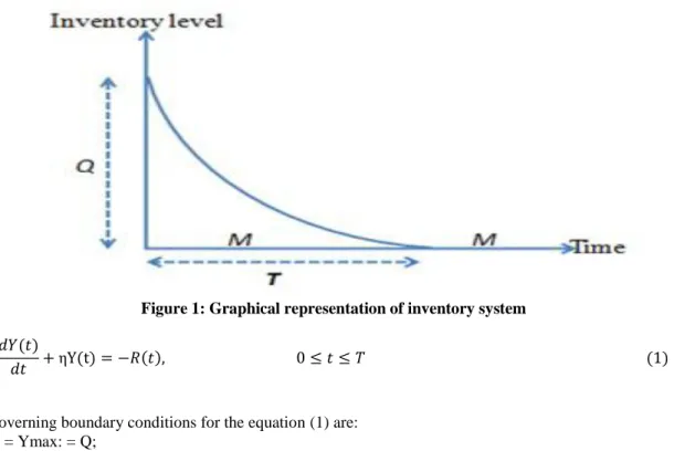
The inventory cycle starts at t = 0 and Q = Ymax units is the initial level of inventory. Due to deterioration and demand, the level of inventory starts reducing. The demand rate is exponentially decreasing with respect to time. Y (t) denotes the instantaneous level of inventory at any time t and the governed differential equation is given as:

Figure 1: Graphical representation of inventory system

𝑑𝑌(𝑡)

𝑑𝑡 +ηY(t) = −𝑅 𝑡 , 0 ≤ 𝑡 ≤ 𝑇 (1)

The governing boundary conditions for the equation (1) are: Y (0) = Ymax: = Q;

Y (t) = 0

and 𝑅 𝑡 = 𝑅0𝑒−𝜑𝑡.

Under these boundary conditions and neglecting the higher powers of theta, the solution of equation (1) is:

𝑌 𝑡 = 𝑅0

η−φ 𝑒η

−φ T−ηt_{− 𝑒}−𝜑𝑡 ₍₂₎

and

𝑌𝑚𝑎𝑥 =

𝑅0

η−φ 𝑒 η−φ T− 1 (3) The cost components are calculated as :

Ordering cost (OC):

𝑂𝐶 = 𝐶(𝑛)

𝑛−1

𝑝=0

𝑒𝑝𝑟𝑡

= 𝐶 𝑛 𝑒𝑟𝐿− 1 1 𝑟𝑇+

𝑟𝑇 4 −1

2 (4)

Inventory holding cost

𝐻𝐶 = 𝐻 𝑛 =𝑅0𝐻(𝑛)

η−φ 𝑒 𝑝𝑟𝑡 𝑛−1

𝑝=0

(𝑒ηT−(η+φ)T_𝑒−𝜑𝑇_)𝑑𝑡 𝑇

0

𝐻𝐶 = 𝑅0𝐻(𝑛) r(φ2_−η2₎ 𝑒

𝑟𝐿

− 1 ηT (5)

Deterioration cost

𝐷𝐶 = 𝐶𝐷 × 𝑁𝑜. 𝑜𝑓 𝐷𝑒𝑡𝑒𝑟𝑖𝑜𝑟𝑎𝑡𝑖𝑛𝑔 𝑢𝑛𝑖𝑡𝑠

𝐷𝐶 = 𝐶𝐷× 𝑌𝑚𝑎𝑥 − 𝑅 (𝑡)𝑑𝑡 𝑇 0

𝐷𝐶 = 𝐶𝐷

𝑅0 η−φ− 1

−1 𝜑 𝑒

𝜑𝑇_{− 1 (6)}

Now, the total cost will be the sum of all the cost components calculated above.

𝑇𝐶 =1

𝑇 𝐻𝐶 + 𝐷𝐶 + 𝑂𝐶

Now we discuss two major cases which arise in each order cycle regarding interest charged and interest earned in detail:

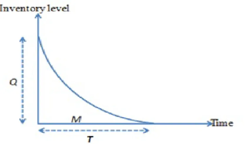
Case1: 𝑴 ≤ 𝒕𝟏

When the credit period is less than or equal to the length of the inventory cycle then the earned interest will be given by 𝑅0𝑝0𝐼𝑒

(𝑒𝑟𝑇−1) 𝑀2

Figure 2: Inventory level for case (1)

In this case total cost will be computed as:

𝑇𝐶1=

1

𝑇[𝑂𝐶 + 𝐻𝐶 + 𝐷𝐶 + 𝐼𝐶1− 𝐼𝐸1]

Solution procedure for the case I:

The procedure follows these steps which are described below : (i) Determine the value of 𝜕𝑇𝐶1

𝜕𝑇

(ii) Check the condition 𝜕 𝑇𝐶1

𝜕𝑇 = 0 and 𝜕2 𝑇𝐶1

𝜕𝑇2 > 0

(iii) Examine the condition given in above step is fulfilled or not, otherwise go to step (i). (iv) Then compute the values of the TC, length of the cycle and ordered quantity.

First and second derivative for case-I are given below:

𝒅𝑻𝑪𝟏

𝒅𝑻 = 𝑐1+ 𝑐2

𝑛_𝑠𝛽 𝑒

𝑟𝐿_{− 1} −2

𝑟 𝑇3+

1 2 𝑇2 +

1

2 𝑅0𝑐𝐷η+ +𝑐0𝑅0𝐼𝑐 𝑐1+ 𝑐2

𝑛_𝑠𝛽

𝜑𝑀 𝑟(η2_−φ2₎

−2M T3 +

1 T2

+ 𝑝0𝑅0𝐼𝑒 𝑒𝑟𝐿− 1

M3_−φM3

𝑟T3 = 0

and

𝒅𝟐_𝑻𝑪 𝟏

𝒅𝑻𝟐 = 𝑐1+

𝑐2

𝑛_𝑠𝛽 𝑒

𝑟𝐿_{− 1} −6

𝑟 𝑇4−

1

𝑇3 + +𝑐0𝑅0𝐼𝑐 𝑐1+

𝑐2

𝑛_𝑠𝛽

𝜑𝑀 𝑟(η2_−φ2₎

−6M T4 +

2 T3

+ 23𝑅0𝐼𝑒

M3_+φM3

𝑟𝑇4 > 0

Minimum solution can be find out by solving 𝒅𝑻𝑪𝟐

𝑅0𝑐𝐷η

2 𝑇

3_{+ 2 𝑐} 1+

𝑐2

𝑛𝑠 𝛽 𝑒

𝑟𝐿_{− 1 +𝑐}

0𝑅0𝐼𝑐 𝑐1+

𝑐2

𝑛𝑠 𝛽

1 (η2_−φ2₎ 𝑒

𝑟𝐿_{− 1 𝜑𝑀 𝑇}

+ 1

𝑟𝑝0𝑅0𝐼𝑒 𝑒

𝑟𝐿_{− 1 M}3_−φM3 ₋2

𝑟 𝑅0 𝑐1+ 𝑐2

𝑛_𝑠𝛽 𝑒

𝑟𝐿_{− 1}

− 2𝑅0 𝑐1+

𝑐2

𝑛_𝑠𝛽 1

(η2_−φ2₎𝐼𝑐 𝑒

𝑟𝐿_{− 1 𝜑𝑀}2_{= 0}

Case II. 𝑴 > 𝒕𝟏

If the credit period extends the length of complete cycle then in this situation, retailer will sell all his items earlier than the scheduled credit period. Therefore, in this case no interest will be taken on the credit. Interest earned in this case, 𝐼𝐸2= 𝑅0𝑝0𝐼𝑒

(𝑒𝑟𝐿−1) 𝑟 𝑀 −

𝑇 2−

𝜑𝑀𝑇 2 . The total cost (TC) can be calculated as follows:

𝑇𝐶2=

1

𝑇[𝑂𝐶 + 𝐻𝐶 + 𝐷𝐶 + 𝐼𝐶2− 𝐼𝐸2]

Solution procedure for the case II:

The procedure follows these steps which are described below : (i) Determine the value of 𝜕𝑇𝐶2

𝜕𝑇

(ii) Check the condition 𝜕 𝑇𝐶2

𝜕𝑇 = 0 and 𝜕2 𝑇𝐶₂

𝜕𝑇2 > 0

(iii) Examine the condition given in above step is fulfilled or not, otherwise go to step (i). (iv) Then compute the values of the TC, length of the cycle and ordered quantity.

Note: Mathematica software has been used in this study for the mathematical calculation. First and second derivative for case-II are given below:

𝒅𝑻𝑪𝟐

𝒅𝑻 = 𝑐1+ 𝑐2

𝑛_𝑠𝛽 𝑒

𝑟𝐿_{− 1} −2

𝑟 𝑇3+

1 2 𝑇2 +

1

2 𝑅0𝑐𝐷η+ 𝑝0𝑅0𝐼𝑒 𝑒

𝑟𝐿_{− 1} 𝑀

Minimum solution can be find out by solving 𝒅𝑻𝑪𝟐

𝒅𝑻 = 𝟎yield

𝑅0𝑐𝐷η

2 𝑇

3₊1

2 𝑐1+ 𝑐2

𝑛_𝑠𝛽 𝑒

𝑟𝐿_{− 1 +} 1

𝑟𝑝0𝑅0𝐼𝑒 𝑒

𝑟𝐿_{− 1 𝑀 𝑇 −}2

𝑟 𝑐1+ 𝑐2

𝑛_𝑠𝛽 𝑒

𝑟𝐿_{− 1 = 0}

IV.

Numerical Example

Case I. (M ≤ T)

If ; 𝑅0 = 100, 𝐼𝑒= 0.14/year, 𝐼𝑐= 0.20/year, η=0.01, 𝜑=0.1, r=0.01, M=15/365 year, 𝑝0=20, 𝑐0=15, L=1,

𝛽=0.23, 𝑐𝐷= 15/unit, 𝑕1=2per unit per item, 𝑕2= 1 per unit per item, 𝑐1=9 per order, 𝑐1=2 per order, 𝑛𝑠 = 5.

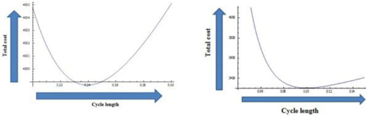
Then, we get the values of TC = 4028=cycle; T = 0:2394, order quantity = 153 units.

Fig 4: Convexity of total cost function CASE II.(M>T)

If ; 𝑅0 = 100, 𝐼𝑒= 0.14/year, 𝐼𝑐= 0.20/year, η=0.01, 𝜑𝛽=0.1, r=0.01, M=36/365 year, 𝑝0=20, 𝑐0=15, L=1,

𝛽=0.23, 𝐶𝐷= 15/unit, 𝑕1=2per unit per item, 𝑕2= 1 per unit per item, 𝑐1=9 per order, 𝑐1=2 per order, 𝑛𝑠 = 5.

Then, we get the values of TC = 3303/cycle; T = 0.091, order quantity = 168 units.

To check the fluctuations of the values, we performed sensitivity analysis. Some tables are listed below to study these changes in the values.

Table-1:

Effect of shipment's number on Total cost, Length of cycle and Ordered quantity:

Parameter (T)Cycle length (Y) Order quantity Total cost (TC)

1 0.2394 153 4560

2 0.2394 153 4303

3 0.2394 153 4173

4 0.2394 153 4089

5 0.2394 153 4028

Table-2: Effect of credit period on Total cost, Length of cycle and Ordered quantity:

Parameter (T)Cycle length (Y) Order quantity Total cost (TC)

5 0.6411 193 4167

10 0.3543 167 4114

15 0.2394 153 4028

Table-3: Effect of Learning rate on Total cost, Length of cycle and Ordered quantity:

Parameter (T)Cycle length (Y) Order quantity Total cost (TC)

0.21 0.1716 113 3882

0.22 0.1639 109 3852

0.23 0.2394 153 4028

0.24 0.2394 153 4010

0.25 0.2394 153 3992

Table-4: Effect of inflation rate on Total cost, Length of cycle and Ordered quantity:

Parameter (T)Cycle length (Y) Order quantity Total cost (TC)

0.01 0.2394 153 4028

0.02 0.2394 153 4045

0.03 0.2392 150 4062

0.04 0.2392 150 4080

0.05 0.2391 148 4097

V.

Observation and Discussion

From the above tables we can study the change of these parameters value on complete cycle length, ordered quantity and Total inventory cost:

(i) Increment in value of number of shipments results in decrement of total cost but does not effect order quantity and cycle length.

(ii) Increment in value of credit period decreases the order quantity and total cost but fluctuate the value of cycle length.

(iii) Increment in the value of learning rate fluctuates the value of total cost value where as order quantity and cycle length first increases then became stable.

(iv) Increase in inflation rate does not put much effect on all three, order quantity, cycle length and Total cost. After observing the above numerical and sensitivity analysis, we found Case:1 to be optimal solution for this model because in case 2, the cycle length is less in comparison to the values of Case-1.

VI.

Conclusion

Many practical factors of regular day life have been associated in this formulated model. Firstly, the factor of decaying of a product is considered into account as the effect of deterioration cannot be neglected in any inventory organization. Secondly, the demand rate is supposed to be exponential and decreasing with the passage of time. Thirdly, the impact of inflation is also incorporated because in the today's world ignorance of this factor is no longer wise. Fourthly, concept of delay in payments is also discussed in the present study. Also, a procedure to solve the cost minimization problem has been discussed. Finally, sensitivity analyses are being done for the two cases to check the effect for the values of cycle length, total cost and order quantity.

Further, many factors like fuzzy environment, alternative demand and deterioration rate can be incorporated in the formulated model for more research.

References

[1]. Aggarwal, A., Sangal, I., and Singh, S. R. (2017). Optimal policy for non-instantaneous decaying inventory model with learning effect with partial shortages. Int J Comput Appl, 161(10), 13-18.

[2]. Aliyu, I., and Sani, B. (2018). An inventory model for deteriorating items with generalised exponential decreasing demand, constant holding cost and time-varying deterioration rate. American Journal of Operations Research, 8(1), 1-16.

[3]. Buzacott, J. A. (1975). Economic order quantities with inflation. Journal of the Operational Research Society, 26(3), 553-558. [4]. Ghare, P. M. and Schrader, G. F. (1963) An inventory model for exponentially deteriorating items', Journal of Industrial

Engineering, 14 (2), 238-243.

[5]. Goyal, S.K. (1985) Economic order quantity under conditions of permissible delay in payments, Journal of Operational Research Society, 36(4), 335-338.

[6]. Jaggi, C. K., Mittal, M., and Khanna, A. (2013). Effects of inspection on retailer's ordering policy for deteriorating items with time-dependent demand under inflationary conditions. International journal of systems science, 44(9), 1774-1782.

[7]. Jayaswal, M., Sangal, I. S. H. A., Mittal, M., and Malik, S. (2019). Effects of learning on retailer ordering policy for imperfect quality items with trade credit financing. Uncertain Supply Chain Management, 7(1), 49-62.

[8]. Khan, M. A. A., Ahmed, S., Babu, M. S., and Sultana, N. (2020). Optimal lot-size decision for deteriorating items with price-sensitive demand, linearly time-dependent holding cost under all-units discount environment. International Journal of Systems

[10]. Kumar, N., and Kumar, S. (2016). Effect of learning and salvage worth on an inventory model for deteriorating items with inventory-dependent demand rate and partial backlogging with capability constraints. Uncertain Supply Chain Management, 4(2), 123-136.

[11]. Kumar, S., and Rajput, U. S. (2015). Fuzzy inventory model for deteriorating items with time dependent demand and partial backlogging. Applied Mathematics, 6(3), 496-509.

[12]. Mandal, B. N., and Phaujdar, S. (1989). A note on an inventory model with stock-dependent consumption rate. Opsearch, 26(1), 43-46.

[13]. Misra, R. B. (1979). A note on optimal inventory management under inflation. Naval Research Logistics Quarterly, 26(1), 161-165. [14]. Mohan, R. (2017). Quadratic demand, variable holding cost with time dependent deterioration without shortages and salvage value.

IOSR J. Math.(IOSR-JM), 13(2), 59-66.

[15]. Moon, I., and Lee, S. (2000). The effects of inflation and time-value of money on an economic order quantity model with a random product life cycle. European Journal of Operational Research, 125(3), 588-601.

[16]. Shah N.H., and Chaudhari U.(2015). Optimal policies for three players with fixed life time and two level trade credit for time and credit dependent demand, Advances in Industrial Engineering and Management, 4(1), 89-100.

[17]. Shah, N.H., Shah D.B., and Patel D.G.,(2013). Optimal transfer, ordering and payment policies for joint supplier buyer inventory model with price-sensitive trapezoidal demand and net credit, International Journal of Systems Science,46(10), 1752-1761. [18]. Singh, D., and Singh, S. R. (2018). Review of Literature and Survey of the Developed Inventory Models, International Journal of

Mathematics and its Applications, 6(1-D),673-685.

[19]. Singh, S. R., and Rathore, H. (2016). A two warehouse inventory model with preservation technology investment and partial backlogging. Scientia Iranica, 23(4), 1952-1958.

[20]. Wright, T. P. (1936) `Factors a_ecting the cost of airplanes', Journal of the aeronautical sciences, 3(4), 122-128.

Jyoti. "Deteriorating Items Inventory Model Having Exponential Declining Demand with

Inflation and Learning Effect under Credit Financing Policy."

IOSR Journal of Mathematics