37
Max-Min Fuzzy Relation Equations for
a Problem of Spatial Analysis
1
Ferdinando Di Martino,
2Salvatore Sessa
1Università degli Studi di Napoli Federico II, Dipartimento di Architettura Via Toledo 402, 80134 Napoli, Italy
2Università degli Studi di Napoli Federico II, Dipartimento di Architettura Via Toledo 402, 80134 Napoli, Italy
Received on: 22-12-2016. Accepted on: 25-01-2017. Published on: 28-02-2017 doi: 10.23755/rm.v31i0.318
© Ferdinando Di Martino and Salvatore Sessa
Abstract
We implement an algorithm that uses a system of max-min fuzzy relation equations (SFRE) for solving a problem of spatial analysis. We integrate this algorithm in a Geographical Information Systems (GIS) tool. We apply our process to determine the symptoms after that an expert sets the SFRE with the values of the impact coefficients related to some parameters of a geographic zone under study. We also define an index of evaluation about the reliability of the results.
Keywords: Fuzzy relation equation, max-min composition, GIS, triangular fuzzy number
38
1.
Introduction
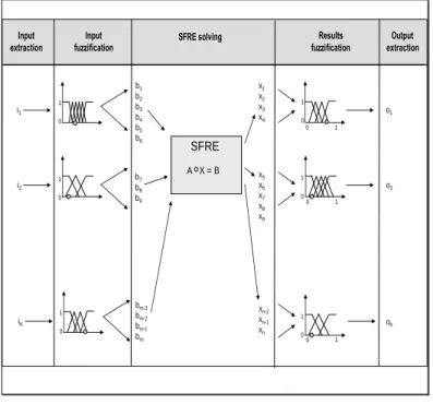
A Geographical Information System (GIS) is used as a support decision system for problems in a spatial domain. We use a GIS to analyse spatial distribution of data, the impact of event data on spatial areas: this analysis implies the creation of geographic thematic maps. Several authors (cfr., e. g., [3], [4], [7], [8], [25]) solve spatial problems using fuzzy relational calculus. In this paper, we propose an inferential method to solve such problems based on an algorithm for the resolution of a system of fuzzy relation equations (shortly, SFRE) given in [20] (cfr. also [21], [22]) and applied in [10] to solve industrial application problems. Here we integrate this algorithm in the context of a GIS architecture. Usually a SFRE with max-min composition is read as
m n mn m
n n
n n
b x a x
a
b x a x
a
b x a x
a
) (
... ) (
...
) (
... ) (
) (
... ) (
1 1
2 2
1 2 1
1 1
1 1 1
(1)
The system (1) is said consistent if it has solutions. Sanchez [23] determines its greatest solution, moreover many researchers have found algorithms which determine minimal solutions of (1) (cfr., e. g., [1], [2], [5], [6], [9], [11]÷[24], [26]). In [20] and [21] a method is described for the consistence of the system (1).
39 Input
extraction
i1 0 1
iK
Input fuzzification
b1
b2
b3
b4
b5
b6
b7
b8
b9
i2
bm-3
bm-2
bm-1
bm
Results fuzzification
0 1
x1
x2
x3
x4
x5
x6
x7
x8
x9
xn-2
xn-1
xn
0 1
Output extraction
o1
o2
oh
SFRE
A X = B
1 0
1 0
1 0 0
1
0 1
0 1
SFRE solving
Fig. 1. Resolution process of a SFRE
The process of the resolution of the system (1) is schematized in Fig. 1. We can determine the maximal interval solutions of (1). Each maximal interval solution is an interval whose extremes are the values taken from a lower solution and from the greatest solution. Every value xi belongs to this interval. If the SFRE (1) is inconsistent, it is possible to determine the rows for which no solution is permitted. If the expert decides to exclude the row for which no solution is permitted, he considers that the symptom bi (for that row) is not relevant to its analysis and it is not taken into account. Otherwise, the expert can modify the setting of the coefficients of the matrix A to verify if the new system has some solution. In general, the SFRE (1) has T maximal interval solutions Xmax(1),…,Xmax(T). In order to describe the extraction process of the solutions, let Xmax(t), t{1,…,T},be a maximal interval solution given below, where Xlow is a lower solution and Xgr is the greatest solution. Our aim is to assign the linguistic label of the most appropriate fuzzy sets, usually triangular fuzzy numbers (briefly, TFN), corresponding to the unknown {
s
j j
j x x
x , ,...,
1
1 } related
to an output variable os, s = 1,…,k. For example, assuming that INF(j), MEAN(j), SUP(j) are the three fundamental values of the generic TFN xj , j=j1, …, js, respectively, we can write their membership functions j1,j2,...,jh as
40
otherwise
0
) ( x
) ( if
) ( )
(
) (
) ( x
) INF(j if 1
1 1
1 1
1
1 1
j1 MEAN j SUP j
j MEAN j
SUP
x j SUP
j MEAN
(2)
} j ,..., {j j and otherwise
0
) ( S x M EAN(j) if
) ( )
( ) (
) ( M x INF(j) if ) ( ) (
) (
1 -s 2
j
UP j
j MEAN j
SUP
x j SUP
j EAN j
INF j MEAN
j INF x
(3)
otherwise
0
) ( x
) ( EAN if
1
) ( x
) ( if ) ( )
(
) (
js s s
s s
s s
s
j SUP j
M
j MEAN j
INF j
INF j
MEAN
j INF x
(4)
If XMint(j) (resp. XMaxt(j)) is the min (resp., max) value of every interval corresponding to the unknown xj, we can calculate the arithmetical mean value XMeant(j) of the j-th component of the above maximal interval solution Xmax(t) as
2
) ( )
( )
(j XMin j XMax j
XMean t t
t
(5)
and we get the vector column XMeant = [XMeant(1),…, XMeant(n)]-1. The value given from max{XMeant(j1),…,XMeant(js)} obtained for the unknowns
s
j
x ,..., x
1
41
k
s
s t
t score o
k O l
1 1
Re (6)
and then as final reliability index of O, the number Rel(O)=max{Relt(O):t=1,…,T}.
The reliability of our solution is higher, the more the final reliability index Rel(O) close to 1 is. In Section 2 we give an overview of how finding the whole set of the solutions of a SFRE. In Section 3 we show how the proposed algorithm is applied in spatial analysis. Section 4 contains the results of our simulation and it is divided in five subsections.
2.
SFRE: An Overview
The SFRE (1) is abbreviated in the following known form:
A ○ X = B where A = (aij), is the matrix of coefficients, X = (x1, x2,…, xn)-1 is the column vector of the unknowns and B = (b1,b2,…,bm)-1 is the column vector of the known terms, being aij, xj, bi [0,1] for each i = 1,…,m and j = 1,…,n. We have the following definitions and terminologies: the whole set of all solutions X of the SFRE (1) is denoted by . A solution Xˆ is called a minimal solution if X ≤Xˆ for someX implies X=Xˆ , where “≤” is the partial order induced in from the natural order of [0, 1]. We also recall that the system (1) has the unique greatest (or maximum) solution Xgr (x1gr,x2gr,...,xngr)1if ≠Ø [23]. A matrix interval Xinterval of the following type:
] , [
[...,...] ] , [
] , [
2 2
1 1
in t
n n erva l
b a
b a
b a
X
where [aj,bj][0,1] for each j=1,…,n, is called an interval solutionof the SFRE (1) if every X=(x1,x2,…,xn)-1 such that xj[aj,bj] for each j = 1,…,n, belongs
42
number of minimal solutions. The SFRE (1) is said to be in normal form if b1≥b2≥…≥bm. The time computational complexity to reduce a SFRE in a normal form is polynomial [20, 22]. Now we consider the matrix A (aij)so defined:
i i i
i
ij
b b b
b
a
ij ij ij *
a if 1
a if
a if 0
where i = 1,…,m and j = 1,…,n, that is aij is S—type coefficient (Smaller) if aij<bi, E—type coefficient (Equal) if aij=bi and G—type coefficient (Greater) if aij>bi. A is called augmented matrix and the system A X B is said associated to the SFRE (1). Without loss of generality, from now on we suppose that the system (1) is in normal form. We also the following definitions and results from [16, 17, 20, 22].
Definition 1. Let SFRE (1) be consistent and
{
1,...,
}
mj j
j
a
a
A
. IfA
jcontains G-type coefficients and k{1,…,m} is the greatest index of row such that akj 1, then the following coefficients in
A
jare called selected:- aij for i{1,…,k} with aij bi bk, - aij for i{k+1,…,m} with aij bi.
Definition 2. If
A
j not contains G-type coefficients, but it contain E-type coefficients and r {1,…,m} is the smallest index of row such that arj br, then any aij bi
in
A
j for i{r,…,m} is called selected.Theorem 1. Let us consider a SFRE (1). Then
- The SFRE (1) is consistent if and only if there exist at least one selected coefficient for each i-th equation, i=1,…,m.
- The complexity time function for determining the consistency of the SFRE (1) is O(m∙n).
43
all the coefficients in the ith equation are not selected and the system is inconsistent. The system is consistent if IND(i) ≠ 0 if for each i = l,...,m and the product
m
i
i IND PN
1
) (
2
gives the upper bound of the number of the eventual minimal solutions.
Theorem 2. Let SFRE (1) be consistent. Then
- the SFRE has an unique greatest solution Xgr with component k gr
j b
x if the jth column
A
j contains selected G-type coefficients akj and xgrj 1 otherwise.- The complexity time function for computing Xgr is O(m∙n).
A help matrix H=[hij], i = 1,…,m and j = 1,…,n, is defined as follows:
otherwise
0
selected is
a if ij
i ij
b
h
Let |Hi| be the number of coefficients hij in the ith equation of the SFRE (1). Then the number of potential minimal solutions cannot exceed the value
m
i i
H PN
1 1
and one has PN2PN1.
Definition 3. Let hi (hi1,hi2,...,hin)and hk (hk1,hk2,...,hkn)be the ith and the
kth rows of the matrix H. If for each j=1,…n, hij 0 implies both hkj 0and ij
kj h
h ,then the ith row (resp. equation) is said dominant over the kth row in H (resp. equation) or that the kth row (resp. equation) is said dominated by the ith row (resp. equation).
If the ith equation is dominant over the kth equation in (1), then the kth equation is a redundant equation of the system. By using Definition 3, we can build a matrix of dimension m×n, called dominance matrix H*, having components:
otherwise
equation another
by dominated
is equation ith
the if 0
*
ij ij
h
44
For eachi= 1, ...,m, now we set |Hi| as the number of coefficients hij bi 0 in the ith row of the dominance matrix H*. When this value is 0, we set |Hi| = 1. Then the number of potential minimal solutions of the SFRE cannot exceed the value
m
i i
H PN
1 *
3
beingPN3PN2PN1 [17, 20 ,22]. There the authors use the symbol j bi
to
indicate the coefficients hij bi 0. We have hij xj bi
if xj[bi,1] and
i
j b
x is the jth component of a minimal solution. A solution of the ith equation can be written as
n
j i i
j b H
1
In [20,22] the concept of concatenation W is introduced to determine all the components of the minimal solutions and it is given by
m
i n
j i m
i i
j b H
W
1 1 1
We can determine the minimal solutions Xlo w(t) (x1lo w(t),x2lo w(t),...,xlo wn (t))1, t{1,...,PN(3)}, with components
otherwise
0
0 b if
bit it
) (
t lo w j
x
In order to determine if a SFRE is consistent, hence its greatest solution and minimal solutions, we have used the universal algorithm of [20,22] based on the above concepts. For brevity of presentation, here we do not give this algorithm which has been implemented and tested under C++ language. The C++ library has been integrated in the ESRI ArcObject Library of the tool ArcGIS 9.3 for a problem of spatial analysis illustrated in the next Section 3.
3.
SFRE in Spatial Analysis
45
We divide this area in P subzones where a subzone is an area in which the same symptoms are derived by input data or facts, and the impact of a symptom on a cause is the same one as well. It is important to note that even if two subzones have the same input data, they can have different impact degrees of symptoms on the causes. For example, the cause that measures the occurrence of floods may be due with different degree of importance to the presence of low porous soils or to areas subjected to continuous rains. Afterwards the area of study is divided in homogeneous subzones, hence the expert creates a fuzzy partition for the domain of each input variable and he determines the values of the symptoms bi, as the membership degrees of the corresponding fuzzy sets (cfr., input fuzzification process of Fig. 1) for each subzone on which the expert sets the most significant equations and the values aij of impact of the j-th cause to the i-th symptom. After i-the determination of i-the set of maximal interval solutions, the expert for each interval solution calculates, for each unknown xj, the mean interval solution Xmean(t) with (5). The linguistic label Relt(os) is assigned to the output variable os . Then he calculates the reliability index Relt(O), given from formula (6), associated to this maximal interval solution t. After the iteration of this step, the expert determines the reliability index (6) for each maximal interval solution, by choosing the output vector O for which Rel(O) assumes the maximum value. Iterating the process for all the subzones (cfr., Fig. 2), the expert can show the thematic map of each output variable. If the SFRE related to a specific subzone is inconsistent, the expert can decide whether or not eliminate rows to find solutions: in the first case, he decides that the symptoms associated to the rows that make the system inconsistent are not considered and eliminates them, so reducing the number of the equations. In the second case, he decides that the corresponding output variable for this subzone remain unknown and it is classified as unknown on the map.
4.
Simulation Results
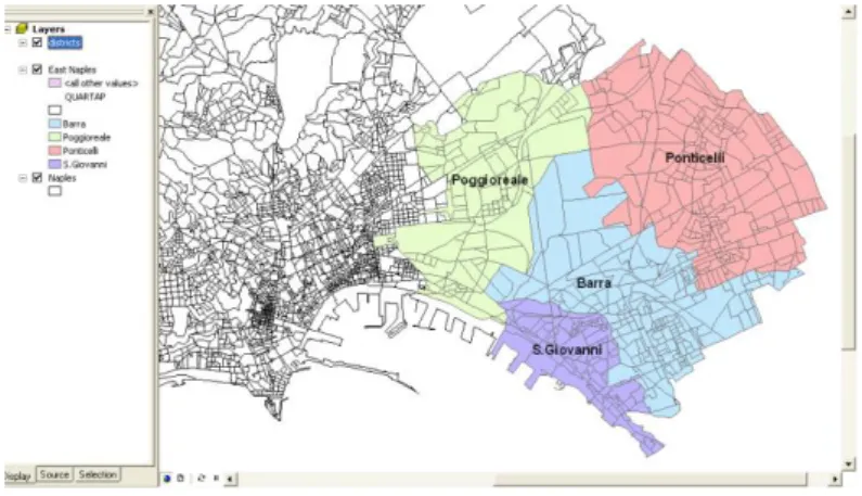
Here we show the results of an experiment in which we apply our method to census statistical data agglomerated on four districts of the east zone of Naples (Italy). We use the year 2000 census data provided by the ISTAT (Istituto Nazionale di Statistica). These data contain informations on population, buildings, housing, family, employment work for each census zone of Naples. Every district is considered as a subzone with homogeneous input data given in Table 2.
In this experiment, we consider the following four output variables: “o1 =
Economic prosperity” (wealth and prosperity of citizens), “o2 = Transition into
46
citizens) and “o4 = Housing development” (presence of building and residential dwellings of new construction). For each variable, we create a fuzzy partition composed by three TFNs called “low”, “mean” and “high” presented in Table 1.
Moreover, we consider the following seven input parameters: i1=percentage of people employed=number of people employed/total work force, i2=percentage of women employed=number of women employed/number of people employed,
Fig. 2. Area of study: four districts at east of Naples (Italy)
Table 1. Values of the TFNs low, mean, high
Output low mean high
INF MEAN SUP INF MEAN SUP INF MEAN SUP
o1 0.0 0.3 0.5 0.3 0.5 0.8 0.5 0.8 1.0
o2 0.0 0.3 0.5 0.3 0.5 0.8 0.5 0.8 1.0
o3 0.0 0.3 0.5 0.3 0.5 0.8 0.5 0.8 1.0
o4 0.0 0.3 0.5 0.3 0.5 0.8 0.5 0.8 1.0
47
buildings built since 1982/total number of residential buildings, i6 = percentage of residential dwellings owned=number of residential dwellings owned/ total number of residential dwellings, i7 = percentage of residential dwellings with central heating system = number of residential dwellings with central heating system/total number of residential dwellings. In Table 4 we show these input data for the four subzones.
Table 2. Input data given for the four subzones
District i1 i2 i3 i4 i5 i6 i7
Barra 0.604 0.227 0.039 0.032 0.111 0.424 0.067 Poggioreale 0.664 0.297 0.060 0.051 0.086 0.338 0.149 Ponticelli 0.609 0.253 0.039 0.042 0.156 0.372 0.159 S. Giovanni 0.576 0.244 0.041 0.031 0.054 0.353 0.097
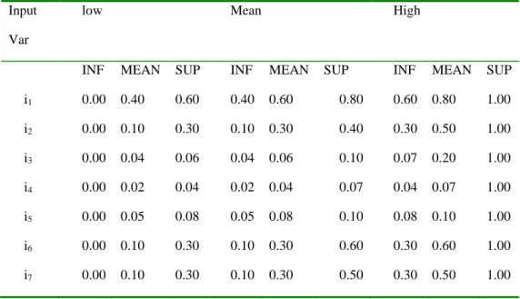
Table 3. TFNs values for the input domains
Input
Var
low Mean High
INF MEAN SUP INF MEAN SUP INF MEAN SUP
i1 0.00 0.40 0.60 0.40 0.60 0.80 0.60 0.80 1.00
i2 0.00 0.10 0.30 0.10 0.30 0.40 0.30 0.50 1.00
i3 0.00 0.04 0.06 0.04 0.06 0.10 0.07 0.20 1.00
i4 0.00 0.02 0.04 0.02 0.04 0.07 0.04 0.07 1.00
i5 0.00 0.05 0.08 0.05 0.08 0.10 0.08 0.10 1.00
i6 0.00 0.10 0.30 0.10 0.30 0.60 0.30 0.60 1.00
48
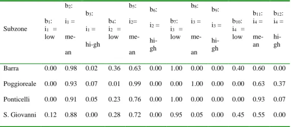
Table 4: TFNs for the symptoms b1 ÷ b12
Subzone b1:
i1 =
low b2:
i1 =
me- an
b3:
i1 =
hi-gh b4:
i2 =
low b5:
i2=
me- an
b6:
i2 =
hi-gh
b7:
i3 =
low b8:
i3 =
me- an
b9:
i3 =
hi-gh
b10:
i4 =
low b11:
i4 =
me-an
b12:
i4 =
hi-gh
Barra 0.00 0.98 0.02 0.36 0.63 0.00 1.00 0.00 0.00 0.40 0.60 0.00 Poggioreale 0.00 0.93 0.07 0.01 0.99 0.00 0.00 1.00 0.00 0.00 0.63 0.37 Ponticelli 0.00 0.91 0.05 0.23 0.76 0.00 1.00 0.00 0.00 0.00 0.93 0.07 S. Giovanni 0.12 0.88 0.00 0.28 0.72 0.00 0.95 0.05 0.00 0.45 0.55 0.00
The expert indicates a fuzzy partition for each input domain formed from three TFNs labeled “low”, “mean” and “high”, whose values are reported in Table 3. In Tables 4 and 5 we show the values of TFNS for the 21 symptoms b1,...,b21. In order to form the SFRE (1) in each subzone, the expert defines the most significant symptoms.
Table 5: TFNs for the symptoms b13 ÷ b21
Subzone
b13: i5 = low
b14: i5 = mean
b15: i5 = high
b16: i6 = low
b17: i6 = mean
b18: i6 = high
b19: i7 = low
b20: i7 = mean
49
4.1 Subzone “Barra”
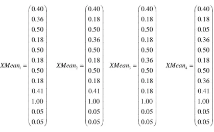
The expert chooses the significant symptoms b2, b4, b5, b7, b10, b11, b15, b17, b18, b19, by obtaining a SFRE (1) with m = 10 equations and n = 12 unknowns. The matrix A of the impact values aij has dimensions 10×12 and the vector B of the symptoms bi has dimension 10×1 and both are given below. The SFRE (1) is inconsistent and eliminating the rows for which the value IND(j) = 0, we obtain four maximal interval solutions Xmax(t) (t=1,…,4) and we calculate the vector column XMeant on each maximal interval solution. Hence we associate to the output variable os (s = 1,…,4), the linguistic label of the fuzzy set with the higher value calculated with formula (5) obtained for the corresponding unknowns s j x ,..., x 1
j and given in Table 6. For determining the reliability of our solutions, we use the index given by formula (6). We obtain that Relt(o1) = Relt(o2) = Relt(o3) = Relt(o4) = 0.6025 for t=1,…,4 and hence Rel(O)=max{Relt(O): t=1,…,4}=0.6025 where O={o1,…o4}. We note that the same final set of linguistic labels associated to the output variables o1 = “high”, o2 = “mean”, o3 = “low”, o4 = “low” is obtained as well. The relevant quantities are given below.
00 . 1 41 . 0 59 . 0 10 . 0 60 . 0 40 . 0 00 . 1 63 . 0 36 . 0 98 . 0 B 0 . 0 1 . 0 0 . 1 0 . 0 3 . 0 4 . 0 0 . 0 3 . 0 4 . 0 0 . 0 2 . 0 5 . 0 5 . 0 4 . 0 2 . 0 5 . 0 5 . 0 1 . 0 4 . 0 4 . 0 1 . 0 4 . 0 4 . 0 1 . 0 3 . 0 7 . 0 3 . 0 1 . 0 5 . 0 2 . 0 1 . 0 4 . 0 1 . 0 2 . 0 5 . 0 2 . 0 3 . 0 3 . 0 1 . 0 1 . 0 1 . 0 2 . 0 1 . 0 2 . 0 1 . 0 1 . 0 1 . 0 1 . 0 1 . 0 2 . 0 1 . 0 3 . 0 7 . 0 2 . 0 3 . 0 7 . 0 3 . 0 3 . 0 7 . 0 3 . 0 0 . 0 0 . 0 1 . 0 1 . 0 4 . 0 6 . 0 1 . 0 4 . 0 6 . 0 1 . 0 3 . 0 5 . 0 0 . 0 0 . 0 3 . 0 2 . 0 2 . 0 8 . 0 1 . 0 3 . 0 8 . 0 0 . 0 2 . 0 0 . 1 0 . 0 0 . 0 0 . 0 2 . 0 7 . 0 2 . 0 2 . 0 7 . 0 2 . 0 2 . 0 7 . 0 2 . 0 0 . 0 0 . 0 0 . 0 2 . 0 6 . 0 3 . 0 4 . 0 5 . 0 4 . 0 2 . 0 5 . 0 3 . 0 2 . 0 3 . 0 1 . 0 3 . 0 7 . 0 2 . 0 2 . 0 0 . 1 0.4 0.0 1.0 0.5 A ] 10 . 0 , 00 . 0 [ ] 10 . 0 , 00 . 0 [ ] 00 . 1 , 00 . 1 [ ] 41 . 0 , 41 . 0 [ ] 36 . 0 , 36 . 0 [ ] 00 . 1 , 00 . 0 [ ] 36 . 0 , 00 . 0 [ ] 00 . 1 , 00 . 0 [ ] 36 . 0 , 36 . 0 [ ] 00 . 1 , 00 . 0 [ ] 36 . 0 , 00 . 0 [ ] 40 . 0 , 40 . 0 [ ] 10 . 0 , 00 . 0 [ ] 10 . 0 , 00 . 0 [ ] 00 . 1 , 00 . 1 [ ] 41 . 0 , 41 . 0 [ ] 36 . 0 , 00 . 0 [ ] 00 . 1 , 00 . 0 [ ] 36 . 0 , 36 . 0 [ ] 00 . 1 , 00 . 0 [ ] 36 . 0 , 00 . 0 [ ] 00 . 1 , 00 . 0 [ ] 36 . 0 , 00 . 0 [ ] 40 . 0 , 40 . 0 [ ] 10 . 0 , 00 . 0 [ ] 10 . 0 , 00 . 0 [ 00 . 1 , 00 . 1 [ ] 41 . 0 , 41 . 0 [ ] 36 . 0 , 00 . 0 [ ] 00 . 1 , 00 . 0 [ ] 36 . 0 , 00 . 0 [ ] 00 . 1 , 00 . 0 [ ] 36 . 0 , 36 . 0 [ ] 00 . 1 , 00 . 0 [ ] 36 . 0 , 00 . 0 [ ] 40 . 0 , 40 . 0 [ ] 10 . 0 , 00 . 0 [ ] 10 . 0 , 00 . 0 [ ] 00 . 1 , 00 . 1 [ ] 41 . 0 , 41 . 0 [ ] 36 . 0 , 00 . 0 [ ] 00 . 1 , 00 . 0 [ ] 36 . 0 , 00 . 0 [ ] 00 . 1 , 00 . 0 [ ] 36 . 0 , 00 . 0 [ ] 00 . 1 , 00 . 0 [ ] 36 . 0 , 36 . 0 [ ] 40 . 0 , 40 . 0 [
50
05 . 0
05 . 0
00 . 1
41 . 0
36 . 0
50 . 0
18 . 0
50 . 0
36 . 0
05 . 0
18 . 0
40 . 0
05 . 0
05 . 0
00 . 1
18 . 0
18 . 0
50 . 0
36 . 0
50 . 0
18 . 0
50 . 0
18 . 0
40 . 0
05 . 0
05 . 0
00 . 1
41 . 0
18 . 0
50 . 0
18 . 0
50 . 0
36 . 0
50 . 0
18 . 0
40 . 0
05 . 0
05 . 0
00 . 1
41 . 0
18 . 0
50 . 0
18 . 0
50 . 0
18 . 0
50 . 0
36 . 0
40 . 0
XMean1 XMean2 XMean3 XMean4
Table 6. Final linguistic labels for the output variables in the district Barra Output variable score1(os) score2(os) score3(os) score4(os)
o1 high high high high
o2 mean mean mean mean
o3 low low low low
o4 low low low low
For determining the reliability of our solutions, we use the index given by formula (6). We obtain Rel(Ok) = 0.4675 for k = 1,..,12. Then we obtain two final sets of linguistic labels associated to the output variables: o1 = “low”, o2 = “low”, o3 = “low”, o4 = “low”, and o1 = “low”, o2 = “low”, o3 = “low”, o4 = “mean”, with a same reliability index value 0.4675. The expert prefers to choose the second solution: o1 = “low”, o2 = “low”, o3 = “low”, o4 = “mean” because he considers that in the last two years in this district the presence of building and residential dwellings of new construction has increased although marginally.
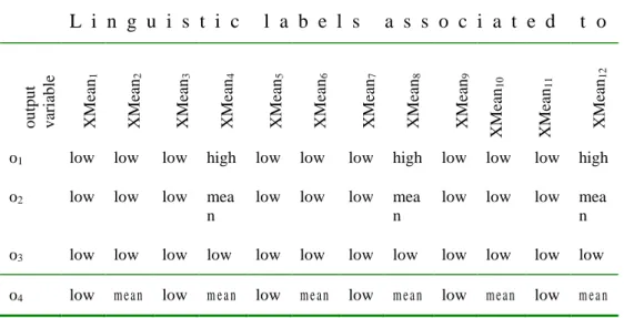
4.2 Subzone “Poggioreale”
51
vector B of the symptoms bi has sizes 11×1 are given below. The SFRE (7) is inconsistent and eliminating the rows for which the value IND(j) = 0, we obtain 12 maximal interval solutions Xmax(t) (t=1,…,12) and we calculate the vector column XMeant on each maximal interval solution. Table 7 contains the output variables and the relevant quantities are given below.
25 . 0 75 . 0 13 . 0 87 . 0 30 . 0 70 . 0 37 . 0 63 . 0 00 . 1 99 . 0 93 . 0 B 2 . 0 6 . 0 3 . 0 1 . 0 2 . 0 1 . 0 1 . 0 2 . 0 1 . 0 1 . 0 2 . 0 1 . 0 0 . 0 3 . 0 7 . 0 1 . 0 3 . 0 5 . 0 3 . 0 5 . 0 8 . 0 0 . 0 1 . 0 4 . 0 4 . 0 1 . 0 0 . 0 5 . 0 2 . 0 1 . 0 5 . 0 2 . 0 1 . 0 5 . 0 1 . 0 0 . 0 2 . 0 8 . 0 2 . 0 2 . 0 8 . 0 2 . 0 1 . 0 9 . 0 1 . 0 1 . 0 9 . 0 1 . 0 2 . 0 1 . 0 0 . 0 6 . 0 4 . 0 2 . 0 6 . 0 4 . 0 3 . 0 6 . 0 4 . 0 2 . 0 1 . 0 2 . 0 1 . 0 3 . 0 7 . 0 2 . 0 3 . 0 7 . 0 3 . 0 3 . 0 7 . 0 3 . 0 1 . 0 0 . 0 0 . 0 6 . 0 5 . 0 3 . 0 6 . 0 5 . 0 3 . 0 6 . 0 5 . 0 4 . 0 2 . 0 2 . 0 1 . 0 3 . 0 7 . 0 2 . 0 3 . 0 7 . 0 3 . 0 3 . 0 7 . 0 3 . 0 0 . 0 0 . 0 0 . 0 2 . 0 0 . 1 2 . 0 2 . 0 0 . 1 2 . 0 2 . 0 0 . 1 2 . 0 0 . 0 0 . 0 0 . 0 2 . 0 9 . 0 2 . 0 2 . 0 0 . 1 2 . 0 2 . 0 0 . 1 2 . 0 2 . 0 3 . 0 1 . 0 3 . 0 7 . 0 2 . 0 2 . 0 0 . 1 0.4 0.0 1.0 0.5 A ] 13 . 0 , 00 . 0 [ ] 25 . 0 , 25 . 0 [ ] 25 . 0 , 00 . 0 [ ] 13 . 0 , 00 . 0 [ ] 13 . 0 , 00 . 0 [ ] 00 . 1 , 00 . 0 [ ] 13 . 0 , 00 . 0 [ ] 13 . 0 , 13 . 0 [ ] 75 . 0 , 75 . 0 [ ] 13 . 0 , 00 . 0 [ ] 30 . 0 , 00 . 0 [ ] 37 . 0 , 37 . 0 [ ] 13 . 0 , 00 . 0 [ ] 25 . 0 , 00 . 0 [ ] 25 . 0 , 25 . 0 [ ] 13 . 0 , 00 . 0 [ ] 13 . 0 , 00 . 0 [ ] 00 . 1 , 00 . 0 [ ] 13 . 0 , 00 . 0 [ ] 13 . 0 , 13 . 0 [ ] 75 . 0 , 75 . 0 [ ] 13 . 0 , 00 . 0 [ ] 30 . 0 , 00 . 0 [ ] 37 . 0 , 37 . 0 [ ] 13 . 0 , 00 . 0 [ ] 25 . 0 , 25 . 0 [ ] 25 . 0 , 00 . 0 [ ] 13 . 0 , 00 . 0 [ ] 13 . 0 , 00 . 0 [ ] 00 . 1 , 00 . 0 [ ] 13 . 0 , 00 . 0 [ ] 13 . 0 , 00 . 0 [ ] 75 . 0 , 75 . 0 [ ] 13 . 0 , 13 . 0 [ ] 30 . 0 , 00 . 0 [ ] 37 . 0 , 37 . 0 [ ] 13 . 0 , 00 . 0 [ ] 25 . 0 , 00 . 0 [ ] 25 . 0 , 25 . 0 [ ] 13 . 0 , 00 . 0 [ ] 13 . 0 , 00 . 0 [ ] 00 . 1 , 00 . 0 [ ] 13 . 0 , 00 . 0 [ ] 13 . 0 , 00 . 0 [ ] 75 . 0 , 75 . 0 [ ] 13 . 0 , 13 . 0 [ ] 30 . 0 , 00 . 0 [ ] 37 . 0 , 37 . 0 [
52 ] 13 . 0 , 00 . 0 [ ] 25 . 0 , 25 . 0 [ ] 25 . 0 , 00 . 0 [ ] 13 . 0 , 00 . 0 [ ] 13 . 0 , 13 . 0 [ ] 00 . 1 , 00 . 0 [ ] 13 . 0 , 00 . 0 [ ] 13 . 0 , 00 . 0 [ ] 75 . 0 , 75 . 0 [ ] 13 . 0 , 00 . 0 [ ] 30 . 0 , 00 . 0 [ ] 37 . 0 , 37 . 0 [ ] 13 . 0 , 00 . 0 [ ] 25 . 0 , 00 . 0 [ ] 25 . 0 , 25 . 0 [ ] 13 . 0 , 00 . 0 [ ] 13 . 0 , 13 . 0 [ ] 0 . 1 , 00 . 0 [ ] 13 . 0 , 00 . 0 [ ] 13 . 0 , 00 . 0 [ ] 75 . 0 , 75 . 0 [ ] 13 . 0 , 00 . 0 [ ] 30 . 0 , 00 . 0 [ ] 37 . 0 , 37 . 0 [ ] 13 . 0 , 00 . 0 [ ] 25 . 0 , 25 . 0 [ ] 25 . 0 , 00 . 0 [ ] 13 . 0 , 00 . 0 [ ] 13 . 0 , 00 . 0 [ ] 00 . 1 , 00 . 0 [ ] 13 . 0 , 00 . 0 [ ] 13 . 0 , 13 . 0 [ ] 75 . 0 , 75 . 0 [ ] 13 . 0 , 00 . 0 [ ] 30 . 0 , 00 . 0 [ ] 37 . 0 , 37 . 0 [ ] 13 . 0 , 00 . 0 [ ] 25 . 0 , 00 . 0 [ ] 25 . 0 , 25 . 0 [ ] 13 . 0 , 00 . 0 [ ] 13 . 0 , 00 . 0 [ ] 00 . 1 , 00 . 0 [ ] 13 . 0 , 00 . 0 [ ] 13 . 0 , 13 . 0 [ ] 75 . 0 , 75 . 0 [ ] 13 . 0 , 00 . 0 [ ] 30 . 0 , 00 . 0 [ ] 37 . 0 , 37 . 0 [
Xmax(5) Xmax(6) Xmax(7) Xmax(8)
] 13 . 0 , 13 . 0 [ ] 25 . 0 , 25 . 0 [ ] 25 . 0 , 00 . 0 [ ] 13 . 0 , 00 . 0 [ ] 13 . 0 , 00 . 0 [ ] 00 . 1 , 00 . 0 [ ] 13 . 0 , 00 . 0 [ ] 13 . 0 , 00 . 0 [ ] 75 . 0 , 75 . 0 [ ] 13 . 0 , 00 . 0 [ ] 30 . 0 , 00 . 0 [ ] 37 . 0 , 37 . 0 [ ] 13 . 0 , 13 . 0 [ ] 25 . 0 , 00 . 0 [ ] 25 . 0 , 25 . 0 [ ] 13 . 0 , 00 . 0 [ ] 13 . 0 , 00 . 0 [ ] 00 . 1 , 00 . 0 [ ] 13 . 0 , 00 . 0 [ ] 13 . 0 , 00 . 0 [ ] 75 . 0 , 75 . 0 [ ] 13 . 0 , 00 . 0 [ ] 30 . 0 , 00 . 0 [ ] 37 . 0 , 37 . 0 [ ] 13 . 0 , 00 . 0 [ ] 25 . 0 , 25 . 0 [ ] 25 . 0 , 00 . 0 [ ] 13 . 0 , 13 . 0 [ ] 13 . 0 , 00 . 0 [ ] 00 . 1 , 00 . 0 [ ] 13 . 0 , 00 . 0 [ ] 13 . 0 , 00 . 0 [ ] 75 . 0 , 75 . 0 [ ] 13 . 0 , 00 . 0 [ ] 30 . 0 , 00 . 0 [ ] 37 . 0 , 37 . 0 [ ] 13 . 0 , 00 . 0 [ ] 25 . 0 , 00 . 0 [ ] 25 . 0 , 25 . 0 [ ] 13 . 0 , 13 . 0 [ ] 13 . 0 , 00 . 0 [ ] 00 . 1 , 00 . 0 [ ] 13 . 0 , 00 . 0 [ ] 13 . 0 , 00 . 0 [ ] 75 . 0 , 75 . 0 [ ] 13 . 0 , 00 . 0 [ ] 30 . 0 , 00 . 0 [ ] 37 . 0 , 37 . 0 [
Xmax(9) Xmax(10) Xmax(11) Xmax(12)
065 . 0 250 . 0 125 . 0 065 . 0 065 . 0 500 . 0 065 . 0 130 . 0 750 . 0 065 . 0 150 . 0 370 . 0 065 . 0 125 . 0 250 . 0 065 . 0 065 . 0 500 . 0 065 . 0 130 . 0 750 . 0 065 . 0 150 . 0 370 . 0 065 . 0 250 . 0 125 . 0 065 . 0 065 . 0 500 . 0 065 . 0 065 . 0 750 . 0 130 . 0 150 . 0 370 . 0 050 . 0 125 . 0 250 . 0 065 . 0 065 . 0 500 . 0 065 . 0 065 . 0 750 . 0 130 . 0 150 . 0 370 . 0
53 065 . 0 250 . 0 125 . 0 065 . 0 130 . 0 500 . 0 065 . 0 065 . 0 750 . 0 065 . 0 150 . 0 370 . 0 065 . 0 125 . 0 250 . 0 065 . 0 130 . 0 500 . 0 065 . 0 065 . 0 750 . 0 065 . 0 150 . 0 370 . 0 050 . 0 250 . 0 125 . 0 065 . 0 065 . 0 500 . 0 130 . 0 065 . 0 750 . 0 065 . 0 150 . 0 370 . 0 05 . 0 125 . 0 250 . 0 065 . 0 065 . 0 500 . 0 130 . 0 065 . 0 750 . 0 065 . 0 150 . 0 370 . 0
XMean5 XMean6 XMean7 XMean8
130 . 0 250 . 0 125 . 0 065 . 0 065 . 0 500 . 0 065 . 0 065 . 0 750 . 0 065 . 0 150 . 0 370 . 0 130 . 0 125 . 0 250 . 0 065 . 0 065 . 0 500 . 0 065 . 0 065 . 0 750 . 0 065 . 0 150 . 0 370 . 0 050 . 0 250 . 0 125 . 0 130 . 0 065 . 0 500 . 0 065 . 0 065 . 0 750 . 0 065 . 0 150 . 0 370 . 0 050 . 0 125 . 0 250 . 0 130 . 0 065 . 0 500 . 0 065 . 0 065 . 0 750 . 0 065 . 0 150 . 0 370 . 0
XMean9 XMean1 0 XMean1 1 XMean1 2
54
Table 7. Final linguistic labels for the output variables in the district “Poggioreale”
L i n g u i s t i c l a b e l s a s s o c i a t e d t o
o
u
tp
u
t
v
ar
iab
le
XM
ea
n1
XM
ea
n2
XM
ea
n3
XM
ea
n4
XM
ea
n5
XM
ea
n6
XM
ea
n7
XM
ea
n8
XM
ea
n9
XM
ea
n10
XM
ea
n11
XM
ea
n12
o1 low low low high low low low high low low low high
o2 low low low mea
n
low low low mea
n
low low low mea
n
o3 low low low low low low low low low low low low
o4 low m e a n low m e a n low m e a n low m e a n low m e a n low m e a n
4.3 Subzone: District Ponticelli
The expert choices the significant symptoms b2, b4, b5, b7, b11, b15, b17, b18, b19, b20, obtaining a SFRE (7) with m = 10 equations and n = 12 variables: The matrix A of sizes 10×12 and the column vector B of dimension 10×1 are given by:
0.30 0.70 0.24 0.76 1.00 0.93 1.00 0.76 0.23 91 . 0
B
1 . 0 5 . 0 3 . 0 0 . 0 2 . 0 1 . 0 0 . 0 2 . 0 1 . 0 0 . 0 2 . 0 1 . 0
0 . 0 2 . 0 7 . 0 1 . 0 2 . 0 4 . 0 1 . 0 2 . 0 4 . 0 0 . 0 1 . 0 2 . 0
2 . 0 1 . 0 0 . 0 2 . 0 1 . 0 0 . 0 2 . 0 1 . 0 0 . 0 2 . 0 1 . 0 0 . 0
3 . 0 7 . 0 3 . 0 2 . 0 8 . 0 2 . 0 2 . 0 8 . 0 2 . 0 3 . 0 7 . 0 3 . 0
0 . 1 1 . 0 0 . 0 7 . 0 3 . 0 1 . 0 7 . 0 3 . 0 1 . 0 0 . 1 1 . 0 0 . 0
0 . 0 3 . 0 1 . 0 1 . 0 8 . 0 2 . 0 1 . 0 9 . 0 3 . 0 1 . 0 8 . 0 4 . 0
0 . 0 1 . 0 3 . 0 2 . 0 2 . 0 8 . 0 0 . 0 1 . 0 0 . 1 0 . 0 2 . 0 0 . 1
0 . 0 0 . 0 0 . 0 2 . 0 8 . 0 2 . 0 2 . 0 8 . 0 2 . 0 2 . 0 8 . 0 2 . 0
0 . 0 0 . 0 0 . 0 0 . 0 1 . 0 2 . 0 0 . 0 1 . 0 2 . 0 0 . 0 1 . 0 2 . 0
2 . 0 3 . 0 1 . 0 3 . 0 7 . 0 2 . 0 2 . 0 0 . 1 0.4 0.0 1.0 0.5
55
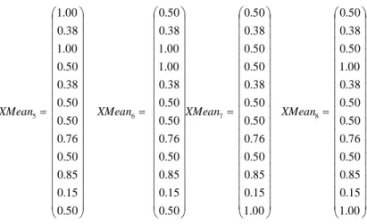
The SFRE (7) is inconsistent and eliminating the rows for which the value IND(j) = 0, we obtain 8 maximal interval solutions Xmax(t) (t=1,…,8) and we calculate the vector column XMeant on each maximal interval solution. Table 10 contains the output variables and the relevant quantities are given below.
] 00 . 1 , 00 . 1 [ ] 30 . 0 , 00 . 0 [ ] 00 . 1 , 70 . 0 [ ] 00 . 1 , 00 . 0 [ ] 76 . 0 , 00 . 0 [ ] 00 . 1 , 00 . 0 [ ] 00 . 1 , 00 . 0 [ ] 76 . 0 , 76 . 0 [ ] 00 . 1 , 00 . 1 [ ] 00 . 1 , 00 . 0 [ ] 76 . 0 , 00 . 0 [ ] 00 . 1 , 00 . 0 [ ] 00 . 1 , 00 . 1 [ ] 30 . 0 , 00 . 0 [ ] 00 . 1 , 70 . 0 [ ] 00 . 1 , 00 . 0 [ ] 76 . 0 , 00 . 0 [ ] 00 . 1 , 00 . 0 [ ] 00 . 1 , 00 . 0 [ ] 76 . 0 , 76 . 0 [ ] 00 . 1 , 00 . 0 [ ] 00 . 1 , 00 . 0 [ ] 76 . 0 , 00 . 0 [ ] 00 . 1 , 00 . 1 [ ] 00 . 1 , 00 . 0 [ ] 30 . 0 , 00 . 0 [ ] 00 . 1 , 70 . 0 [ ] 00 . 1 , 00 . 0 [ ] 76 . 0 , 00 . 0 [ ] 00 . 1 , 00 . 0 [ ] 00 . 1 , 00 . 0 [ ] 76 . 0 , 76 . 0 [ ] 00 . 1 , 00 . 1 [ ] 00 . 1 , 00 . 1 [ ] 76 . 0 , 00 . 0 [ ] 00 . 1 , 00 . 0 [ ] 00 . 1 , 00 . 0 [ ] 30 . 0 , 00 . 0 [ ] 00 . 1 , 70 . 0 [ ] 00 . 1 , 00 . 0 [ ] 76 . 0 , 00 . 0 [ ] 00 . 1 , 00 . 0 [ ] 00 . 1 , 00 . 0 [ ] 76 . 0 , 76 . 0 [ ] 00 . 1 , 00 . 0 [ ] 00 . 1 , 00 . 1 [ ] 76 . 0 , 00 . 0 [ ] 00 . 1 , 00 . 1 [
Xmax (1) Xmax (2) Xmax (3) Xmax (4)
] 00 . 1 , 00 . 1 [ ] 30 . 0 , 00 . 0 [ ] 00 . 1 , 70 . 0 [ ] 00 . 1 , 00 . 0 [ ] 76 . 0 , 76 . 0 [ ] 00 . 1 , 00 . 0 [ ] 00 . 1 , 00 . 0 [ ] 76 . 0 , 00 . 0 [ ] 00 . 1 , 00 . 1 [ ] 00 . 1 , 00 . 0 [ ] 76 . 0 , 00 . 0 [ ] 00 . 1 , 00 . 0 [ ] 00 . 1 , 00 . 1 [ ] 30 . 0 , 00 . 0 [ ] 00 . 1 , 70 . 0 [ ] 00 . 1 , 00 . 0 [ ] 76 . 0 , 76 . 0 [ ] 00 . 1 , 00 . 0 [ ] 00 . 1 , 00 . 0 [ ] 76 . 0 , 00 . 0 [ ] 00 . 1 , 00 . 0 [ ] 00 . 1 , 00 . 0 [ ] 76 . 0 , 00 . 0 [ ] 00 . 1 , 00 . 1 [ ] 00 . 1 , 00 . 0 [ ] 30 . 0 , 00 . 0 [ ] 00 . 1 , 70 . 0 [ ] 00 . 1 , 00 . 0 [ ] 76 . 0 , 76 . 0 [ ] 00 . 1 , 00 . 0 [ ] 00 . 1 , 00 . 0 [ ] 76 . 0 , 00 . 0 [ ] 00 . 1 , 00 . 1 [ ] 00 . 1 , 00 . 1 [ ] 76 . 0 , 00 . 0 [ ] 00 . 1 , 00 . 0 [ ] 00 . 1 , 00 . 0 [ ] 30 . 0 , 00 . 0 [ ] 00 . 1 , 70 . 0 [ ] 00 . 1 , 00 . 0 [ ] 76 . 0 , 76 . 0 [ ] 00 . 1 , 00 . 0 [ ] 00 . 1 , 00 . 0 [ ] 76 . 0 , 00 . 0 [ ] 00 . 1 , 00 . 0 [ ] 00 . 1 , 00 . 1 [ ] 76 . 0 , 00 . 0 [ ] 00 . 1 , 00 . 1 [
Xmax(5) Xmax(6) Xmax(7) Xmax(8)
00 . 1 15 . 0 85 . 0 50 . 0 38 . 0 50 . 0 50 . 0 76 . 0 00 . 1 50 . 0 38 . 0 50 . 0 00 . 1 15 . 0 85 . 0 50 . 0 38 . 0 50 . 0 50 . 0 76 . 0 50 . 0 50 . 0 38 . 0 00 . 1 50 . 0 15 . 0 85 . 0 50 . 0 38 . 0 50 . 0 50 . 0 76 . 0 00 . 1 00 . 1 38 . 0 5 . 0 50 . 0 15 . 0 85 . 0 50 . 0 38 . 0 50 . 0 50 . 0 76 . 0 50 . 0 00 . 1 38 . 0 00 . 1
56
00 . 1
15 . 0
85 . 0
50 . 0
76 . 0
50 . 0
50 . 0
38 . 0
00 . 1
50 . 0
38 . 0
50 . 0
00 . 1
15 . 0
85 . 0
50 . 0
76 . 0
50 . 0
50 . 0
38 . 0
50 . 0
50 . 0
38 . 0
50 . 0
50 . 0
15 . 0
85 . 0
50 . 0
76 . 0
50 . 0
50 . 0
38 . 0
00 . 1
00 . 1
38 . 0
50 . 0
50 . 0
15 . 0
85 . 0
50 . 0
76 . 0
50 . 0
50 . 0
38 . 0
50 . 0
00 . 1
38 . 0
00 . 1
XMean5 XMean6 XMean7 XMean8
Now we associate to the output variables os k = 1,…,4, the linguistic label of the fuzzy set with the higher XMeanj obtained for the corresponding unknowns
1
j x ,…,
s
j
x obtaining:
Table 8. Final linguistic labels for the output variables in the district “Ponticelli”
L i n g u i s t i c l a b e l s a s s o c i a t e d t o
output varia
ble
XM
ea
n1
XM
ea
n2
XMe
an3
XMe
an4
XMe
an5
XMe
an6
XMe
an7
XMe
an8
o1 Low-high high low Low
-high -high Low high low Low-high
o2 mean low mea
n
low Low -high
low Low
-high low
o3 Low-high Low-high Low
-high -high Low mean mean mean mean
o4 low low low low low low low low
57
= 0.565 Rel(O4) = 0.5, Rel(O5) =0.565, Rel(O6) = 0.69, Rel(O7) = 0.565 Rel(O8) = 0.565.
Thus we choice the solution O6 which have the greatest reliability Rel(O6) = 0.69. Our solution for this subzone is: o1 = “high”, o2 = “low”, o3 = “mean”, o4 = “low”.
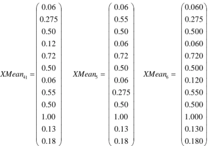
4.4Subzone: district S. Giovanni
The expert choices the significant symptoms b2, b4, b5, b7, b11, b15, b17, b18, b19, b20, obtaining a SFRE (1) with m = 12 equations and n = 12 variables: The matrix A of sizes 12×12 and the column vector B of sizes 12×1 are given by:
0 . 1 18 . 0 0.82 0.13 0.87 0.55 0.45 0.95 0.72 0.28 0.88 12 . 0 B 0 . 0 0 . 0 0 . 1 0 . 0 1 . 0 4 . 0 0 . 0 1 . 0 4 . 0 1 . 0 2 . 0 5 . 0 5 . 0 1 . 0 0 . 0 1 . 0 0 . 0 0 . 0 1 . 0 0 . 0 0 . 0 1 . 0 0 . 0 0 . 0 1 . 0 7 . 0 3 . 0 3 . 0 6 . 0 3 . 0 3 . 0 6 . 0 3 . 0 3 . 0 6 . 0 3 . 0 1 . 0 4 . 0 1 . 0 0 . 0 1 . 0 0 . 0 0 . 0 1 . 0 0 . 0 0 . 0 1 . 0 0 . 0 0 . 0 2 . 0 8 . 0 1 . 0 2 . 0 5 . 0 1 . 0 2 . 0 5 . 0 1 . 0 3 . 0 6 . 0 0 . 0 2 . 0 0 . 0 2 . 0 8 . 0 2 . 0 2 . 0 5 . 0 2 . 0 2 . 0 6 . 0 3 .. 0 0 . 0 1 . 0 2 . 0 1 . 0 3 . 0 6 . 0 1 . 0 3 . 0 5 . 0 1 . 0 3 . 0 5 . 0 0 . 0 1 . 0 3 . 0 0 . 0 1 . 0 9 . 0 0 . 0 1 . 0 0 . 1 0 . 0 2 . 0 0 . 1 0 . 0 2 . 0 0 . 0 2 . 0 8 . 0 2 . 0 2 . 0 8 . 0 2 . 0 2 . 0 8 . 0 2 . 0 0 . 0 0 . 0 2 . 0 0 . 0 1 . 0 4 . 0 0 . 0 1 . 0 4 . 0 0 . 0 1 . 0 4 . 0 0 . 0 3 . 0 0 . 0 1 . 0 9 . 0 1 . 0 1 . 0 9 . 0 1 . 0 1 . 0 9 . 0 1 . 0 0 . 0 0 . 0 1 . 0 0 . 0 1 . 0 3 . 0 0 . 0 1 . 0 0.3 0.0 0.1 0.3 A
58 ] 18 . 0 , 18 . 0 [ ] 13 . 0 , 13 . 0 [ ] 00 . 1 , 00 . 1 [ ] 00 . 1 , 00 . 0 [ ] 55 . 0 , 00 . 0 [ ] 12 . 0 , 00 . 0 [ ] 00 . 1 , 00 . 0 [ ] 72 . 0 , 72 . 0 [ ] 12 . 0 , 12 . 0 [ ] 00 . 1 , 00 . 0 [ ] 55 . 0 , 55 . 0 [ ] 12 . 0 , 00 . 0 [ ] 18 . 0 , 18 . 0 [ ] 13 . 0 , 13 . 0 [ ] 00 . 1 , 00 . 1 [ ] 00 . 1 , 00 . 0 [ ] 55 . 0 , 55 . 0 [ ] 12 . 0 , 00 . 0 [ ] 00 . 1 , 00 . 0 [ ] 72 . 0 , 72 . 0 [ ] 12 . 0 , 00 . 0 [ ] 00 . 1 , 00 . 0 [ ] 55 . 0 , 00 . 0 [ ] 12 . 0 , 12 . 0 [ ] 18 . 0 , 18 . 0 [ ] 13 . 0 , 13 . 0 [ ] 00 . 1 , 00 . 1 [ ] 00 . 1 , 00 . 0 [ ] 55 . 0 , 00 . 0 [ ] 12 . 0 , 00 . 0 [ ] 00 . 1 , 00 . 0 [ ] 72 . 0 , 72 . 0 [ ] 12 . 0 , 00 . 0 [ ] 00 . 1 , 00 . 0 [ ] 55 . 0 , 55 . 0 [ ] 12 . 0 , 12 . 0 [
max (1) max ,(2) max ,(3)
X X
X ] 18 . 0 , 18 . 0 [ ] 13 . 0 , 13 . 0 [ ] 00 . 1 , 00 . 1 [ ] 00 . 1 , 00 . 0 [ ] 55 . 0 , 55 . 0 [ ] 12 . 0 , 12 . 0 [ ] 00 . 1 , 00 . 0 [ ] 72 . 0 , 72 . 0 [ ] 12 . 0 , 00 . 0 [ ] 00 . 1 , 00 . 0 [ ] 55 . 0 , 00 . 0 [ ] 12 . 0 , 00 . 0 [ ] 18 . 0 , 18 . 0 [ ] 13 . 0 , 13 . 0 [ ] 00 . 1 , 00 . 1 [ ] 00 . 1 , 00 . 0 [ ] 55 . 0 , 00 . 0 [ ] 12 . 0 , 12 . 0 [ ] 00 . 1 , 00 . 0 [ ] 72 . 0 , 72 . 0 [ ] 12 . 0 , 00 . 0 [ ] 00 . 1 , 00 . 0 [ ] 55 . 0 , 55 . 0 [ ] 12 . 0 , 00 . 0 [ ] 18 . 0 , 18 . 0 [ ] 13 . 0 , 13 . 0 [ ] 00 . 1 , 00 . 1 [ ] 00 . 1 , 00 . 0 [ ] 55 . 0 , 55 . 0 [ ] 12 . 0 , 00 . 0 [ ] 00 . 1 , 00 . 0 [ ] 72 . 0 , 72 . 0 [ ] 12 . 0 , 12 . 0 [ ] 00 . 1 , 00 . 0 [ ] 55 . 0 , 00 . 0 [ ] 12 . 0 , 00 . 0 [
max (4) max (5) max (6)
X X
X 18 . 0 13 . 0 00 . 1 50 . 0 275 . 0 06 . 0 50 . 0 72 . 0 12 . 0 50 . 0 55 . 0 06 . 0 18 . 0 13 . 0 00 . 1 50 . 0 55 . 0 06 . 0 50 . 0 72 . 0 06 . 0 50 . 0 275 . 0 12 . 0 18 . 0 13 . 0 00 . 1 50 . 0 275 . 0 06 . 0 50 . 0 72 . 0 06 . 0 50 . 0 55 . 0 12 . 0
1 2 3
XMean XMean
59
180 . 0
130 . 0
000 . 1
500 . 0
550 . 0
120 . 0
500 . 0
720 . 0
060 . 0
500 . 0
275 . 0
060 . 0
18 . 0
13 . 0
00 . 1
50 . 0
275 . 0
06 . 0
50 . 0
72 . 0
06 . 0
50 . 0
55 . 0
06 . 0
18 . 0
13 . 0
00 . 1
50 . 0
55 . 0
06 . 0
50 . 0
72 . 0
12 . 0
50 . 0
275 . 0
06 . 0
41 5 6
XMean XMean
XMean
Table 9. Final linguistic labels for the output variables in the district “San Giovanni”
output variabl e
linguistic label associate
d to
XMean1
linguistic label associate
d to
XMean2
linguistic label associate
d to
XMean3
linguistic label associate
d to
XMean4
linguistic label associate
d to
XMean5
linguistic label associate
d to
XMean6
o1 mean high mean high mean high
o2 mean mean mean mean mean mean
o3 high mean high mean high mean
o4 low low low low low low
60
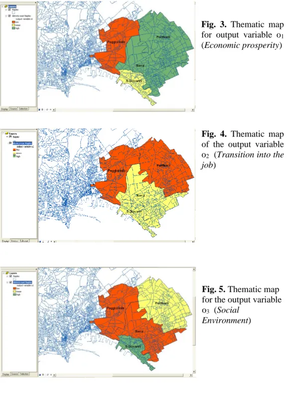
4.5Thematic maps and conclusions
Finally, we obtain four final thematic maps shown in Figs. 3, 4, 5, 6 for the output variable o1, o2, o3, o4, respectively.
Fig. 3. Thematic map for output variable o1
(Economic prosperity)
Fig. 4. Thematic map of the output variable
o2 (Transition into the
job)
Fig. 5. Thematic map for the output variable o3 (Social
61
Fig. 6. Thematic map for the output variable
o4 (Housing
development)
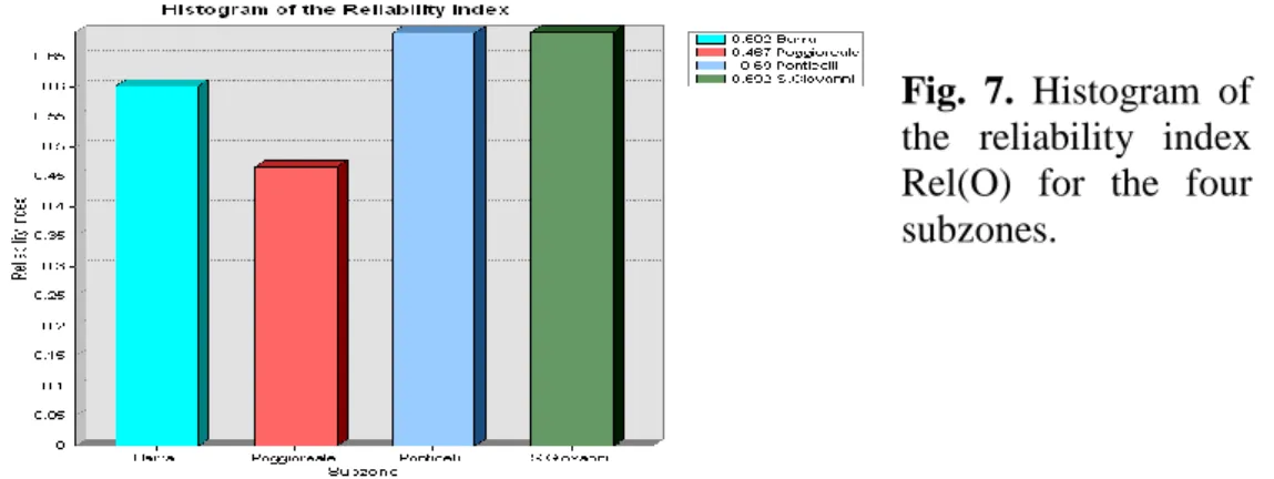
The results show that there was no housing development in the four districts in the last 10 years and there is difficulty in finding job positions. In Fig. 7 we show the histogram of the reliability index Rel(O) for each subzone, where O=[o1,o2,o3,o4].
Fig. 7. Histogram of the reliability index Rel(O) for the four subzones.
This paper is a new reformulation of our work titled “Spatial Analysis and Fuzzy Relation Equations” published in Advances in Fuzzy Systems,
Volume 2011 (2011), Article ID 429498, 14 pages
62
References
1. Chen, L., Wang, P.: Fuzzy Relational Equations (I): the General and Specialized Solving Algorithms. Soft Computing 6, 428—435 (2002)
2. De Baets, B.: Analytical Solution Methods for Fuzzy Relational Equations. In: Dubois, D., Prade, H., (eds.) Fundamentals of Fuzzy Sets, The Handbooks of Fuzzy Sets Series, Vol. 1, pp. 291—340. Kluwer Academic Publishers, Dordrecht (2000)
3. Di Martino, F., Loia, V., Sessa, S.: A Fuzzy-Based Tool for Modelization and Analysis of the Vulnerability of Aquifers: a Case Study. International Journal of Approximate Reasoning 38, 98—111 (2005)
4. Di Martino, F., Loia, V., Sessa, S., Giordano, M.: An Evaluation of the Reliability of a GIS Based on the Fuzzy Logic in a Concrete Case Study. In: Petry, F.E., Robinson,V.B., Cobb, M.A. (eds.) Fuzzy Modeling with Spatial Information for Geographic Problems, pp. 185—208. Springer, Heidelberg (2005)
5. Di Martino, F., Loia, V., Sessa, S.: Extended Fuzzy C-Means Clustering Algorithm for Hotspot Events in Spatial Analysis, International Journal of Hybrid Intelligent Systems 5 (1), 31—44 (2008)
6. Di Nola, A., Pedrycz, W., Sessa, S., Sanchez, E.: Fuzzy Relation Equations and Their Application to Knowledge Engineering. Kluwer Academic Press, Dordrecht, 1989
7. Groenemans, R., Van Ranst, E., Kerre, E.: Fuzzy Relational Calculi in Land Evaluation. Geoderma 77 (2-4), 283—298 (1997)
8. Hemetsberger, M., Klinger, G., Niederer, S., Benedikt, J.: Risk Assessment of Avalanches - a Fuzzy GIS Application. In: Ruan, D., D’hondt, P., Kerre, E.E. (eds.) Proceedings of 5th International FLINS. Conference Computational Intelligent Systems for Applied Research, pp. 397—402. World Scientific, Singapore (2002)
9. Higashi, M., Klir, G.J.: Resolution of Finite Fuzzy Relation Equations. Fuzzy Sets and Systems 13 (1), 65—82 (1984)
63
of 5th International Conference Textile Science TEXSCI 2003. CD ROM Edition. Liberec, (2003)
11. Li, P., Fang, S.C..: A Survey on Fuzzy Relational Equations, Part I: Classification and Solvability. Fuzzy Optimation and Decision Making 8, 179—229 (2009)
12. Markovskii, A.V. : On the Relation between Equations with Max-Product Composition and the Covering Problem. Fuzzy Sets and Systems 153, 261— 273 (2005)
13. Miyakoshi, M., Shimbo, M.: Minimal Solutions of Systems of Fuzzy Equations. Fuzzy Sets and Systems 19, (1986) 37—46
14. Pappis, C.P., Adamopoulos, G.: A Computer Algorithm for the Solution of the Inverse Problem of Fuzzy Systems. Fuzzy Sets and Systems 39, 279—290 (1991)
15. Pappis, C.P., Sugeno, M.: Fuzzy Relational Equations and the Inverse Problem. Fuzzy Sets and Systems 15, 79—90 (1985)
16. Peeva, K.: Systems of Linear Equations over a Bounded Chain. Acta Cybernetica 7(2), 195-202 (1985)
17. Peeva, K.: Fuzzy Linear Systems. Fuzzy Sets and Systems 49, 339—355 (1992)
18. Peeva, K.: Fuzzy Linear Systems –Theory and Applications in Artificial Intelligence Areas, DSc Thesis, Sofia (2002) (in Bulgarian)
19. Peeva, K.: Resolution of Min–Max Fuzzy Relational Equations. In: Nikravesh, M., Zadeh , L.A., Korotkikh, V. (eds.) Fuzzy Partial Differential Equations and Relational Equations, pp. 153—166. Springer, Heidelberg (2004)
20. Peeva, K.: Universal Algorithm for Solving Fuzzy Relational Equations. Italian Journal of Pure and Applied Mathematics 19, 9—20 (2006)
64
22. Peeva, K., Kyosev, Y.: Fuzzy Relational Calculus: Theory, Applications and Software (with CD-ROM). Series Advances in Fuzzy Systems-Applications and Theory, vol. 22, World Scientific, Singapore (2004)
23. Sanchez, E.: Resolution of Composite Fuzzy Relation Equations. Information and Control, 30, 38—48 (1976)
24. Shieh, B.S.: New Resolution of Finite Fuzzy Relation Equations with Max-Min Composition. Internat. J. of Uncertainty, Fuzziness Knowledge Based Systems 16 (1), 19—33 (2008)
25. Sicat,, R.S., Carranza, E.J.M., Nidumolu, U.B.: Fuzzy modeling of farmers’ kno- wledge for land suitability classification. Agricultural Systems 83, 49—75 (2005)