On modified skew logistic regression model and its applications

ON MODIFIED SKEW LOGISTIC REGRESSION MODEL AND

ITS APPLICATIONS

C. Satheesh Kumar1

Department of Statistics, University of Kerala, Trivandrum-695 581, India L. Manju

Department of Community Medicine, Sree Gokulam Medical College, Trivandrum-695 607, India

1. Introduction

Regression methods are usually used for studying the relationship between a re-sponse variable and one or more explanatory variables. Over the last decade the logistic regression model, also known as logit model, has become the standard method of analysis when the outcome variable is dichotomous in nature and it has been found applications in several areas of scientific studies such as bioassay problems (Finney, 1952), study of income distributions (Fisk, 1961), analysis of survival data (Plackett, 1959) and modelling of the spread of an innovation (Oliver, 1969). The main drawback of a logit model is that it consider variables of only symmetric and unimodal nature. But asymmetry may arise in several practical situations where the logit model is not appropriate. So through this paper we develop certain regression models based on a modified version of the skew-logistic distribution and compare it with the existing logit model as well as a regression model based on the skew-logistic distribution of (Nadarajah, 2009).

The paper is organized as follows. In section 2, we describe some important aspects of the skew-logistic regression model(SLRM) and propose a modified ver-sion of the SLRM, which we termed as the “Modified Skew Logistic Regresver-sion Model (MSLRM)”. In section 3, we obtain some structural properties of the mod-ified skew logistic distribution. In section 4, we consider the estimation of the parameters of the MSLRM and in section 5, two real life medical datasets are considered for illustrating the usefulness of the model compared to both the logit and skew logit models. In section 6, a generalized likelihood ratio test procedure is suggested for testing the significance of the parameters and a simulation study is also conducted to test the efficiency of the maximum likelihood estimators(MLEs) of MSLRM.

2. Skew Logistic and Modified Skew Logitic regression models

A random variable X is said to follow the logistic distribution (LD) if its probability density function (p.d.f) is of the following form.

f(x) = e −_x

(1 +e−x₎2, (1)

wherex∈ R= (−∞, +∞). The logistic regression model(LRM) is given by

p= 1

1 +e−z, (2)

in which

z=a+ s

X

r=1

brXr. (3)

The importance of the logistic regression model is due to its mathematical flexibility and in several medical applications it provides clinically meaningful in-terpretations (Hosmer and Lemeshow, 2000). Nadarajah (2009) developed a mod-ified version of the logistic distribution, similar to the skew-normal distribution of Azzalini (1985), namely skew-logistic distribution(SLD), which he defined through the following p.d.f, in which x∈R, β >0 andλ∈R.

f(x) = 2e(

−x

β)

βh1 +e( −x

β ) i2h

1 +e( −λx

β )

i (4)

When λ = 0, (4) reduces to p.d.f of the standard logistic distribution given in (1). The main feature of skew-logistic distribution is that a new parameter λ is included here for controlling the skewness and kurtosis. Now the skew-logistic regression model (SLRM) can be obtained through the following double series representation.

p=

          

2 ∞

P

j=0 ∞

P

=0 −₁

j

−₂ k

1

1+λ+λj+ke(

(1+λ+λj+k)z

β ) _{if z <}0

1−2 ∞

P

j=0 ∞

P

=0 −1

j

−2 k

1

1+λj+ke

−((1+λj+k)z

β ) if z >0

(5)

where z is as defined in (3). Here we consider a modified version of the skew-logistic distribution namely “the modified skew-logistic distribution(MSLD)” through the following p.d.f, in whichx∈R,α≥ −1 andβ >0.

f(x;α, β) = 2 α+ 2

e−x (1 +e−x₎2

1 + αe −βx 1 +e−_βx

(6)

density given in (4). The p.d.ff(x;α, β) of theM SLD(α, β) can also be expressed interms of the following single series as well as double series representations,

f(x;α, β) =

                   2 α+2   e−x

(1+e−x₎2 + α

∞

P j=0(

−1

j)e

(−1+βj)x

(1+e−x₎2



, if x <0

2 α+2

  e−x

(1+e−x₎2 + α

∞

P j=0(

−1

j)e

−(1+β+βj)x

(1+e−x₎2



, if x >0

(7)

f(x;α, β) =

               2 α+2 " ∞ P k=0 −2 k

e(1+k)x+α ∞ P j=0 ∞ P k=0 −1 j −2 k

e(1+βj+k)x

#

, if x <0

2 α+2 " ∞ P k=0 −₂ k

e−(1+k)x_+α ∞ P j=0 ∞ P k=0 −₁ j −₂ k

e−(1+β+βj+k)x

#

, if x >0 (8)

The modified skew-logistic regression model(MLRM) is given by the following double series representation based on (8).

p=                    2 α+2 " ∞ P k=0 −2 k

_e(1+k)z

(1+k) +α ∞ P j=0 ∞ P k=0 −1 j −2 k

_e(1+βj+k)z

(1+βj+k)

#

, if z <0

1− 2 α+2 " ∞ P k=0 −₂ k

_e−(1+k)z

(1+k) +α ∞ P j=0 ∞ P k=0 −₁ j −₂ k

_e−(1+β+βj+k)z

(1+β+βj+k)

#

, if z≥0 (9)

where z is as given in (3). For the derivation of (9), see Appendix I. A graphical representation of MSLRM for particular values ofαandβ = 2 is given in Figure 1.

3. Some structural properties of modified skew logistic model

Proposition 1. If X follows M SLD(α, β), then Y = −X follows a convex mixture of standard logistic and skew-logistic distributions.

Proof. The p.d.ff(y)of Y is the following , fory∈R ,β∈R andα≥ −1.

f(y) =f(−y;α, β)dx dy = 2 α+2 ey

(1+ey₎2

h

1 +α₁₊eβy_eβy i

= _α+22 ₍₁₊e_e−−yy₎2

h

1 +_1+eα−βy i

= _α+22 ₍₁₊e_e−−yy₎2 + 2α α+2

e−y

Figure 1 – Plots of regression function of M SLD(α,2) for different values ofα.

which shows that the p.d.f of Y can be considered as a convex mixture of the p.d.f of the standard logistic and and skew-logistic distributions.

Proposition 2. If X followsM SLD(α, β), thenY =|X|follows a half logis-tic distribution.

Proof. Fory >0, the p.d.f f(y)of Y is

f(y) =f(y;α, β)dx_dy+f(−y;α, β)dx_dy

= _α+22 ₍₁₊e_e−−yy₎2

h

1 +α₁₊e−_eβy−βy i

+_α+22 ₍₁₊e_e−−yy₎2

h

1 + _1+eα−βy i

=₍₁₊2e_e−−yy₎2,

which is the p.d.f of the half logistic distribution.

Proposition 3. If X follows M SLD(α, β), then Y =X1/c, c∈(0,1]follows a distribution with p.d.f

f(y) = 2c α+ 2

yc−1_e−yc

(1 +e−yc

)2

1 +α e −βyc

1 +e−_βyc

Proof. For anyy >0, the p.d.f f(y)ofY =X1/c is given by

f(y) =_α+22 yc −1

e−yc

(1+e−yc₎2

h

1 +α₁₊e−_e−βycβyci

dx dy

=_α2₊₂c ₍₁₊yc−_e1−e−ycyc₎2

h

Proposition 4. The first four raw moments of M SLD(α, β)are given by

µ′ 1=

2α α+ 2

∞ X j=0 ∞ X k=0 −1 j −2 k " 1

(1 +β+βj+k)2 +

(−1) (1 +βj+k)2

#

, (10)

µ′ 2=

4 α+ 2

  2 ∞ X k=0 −₂ k

(1 +k)3 +α ∞ X j=0 ∞ X k=0 −1 j −2 k " 1

(1 +β+βj+k)3 +

1 (1 +βj+k)3

#_

, (11)

µ′ 3=

12α α+ 2

∞ X j=0 ∞ X k=0 ₋₁ j ₋₂ k " ₁

(1 +β+βj+k)4+

(−1) (1 +βj+k)4

# (12) and µ′ 4= 48 α+ 2

  2 ∞ X k=0 −2 k

(1 +k)5 +α ∞ X j=0 ∞ X k=0 −1 j −2 k " 1

(1 +β+βj+k)5 +

1 (1 +βj+k)5

#_

.(13)

Proof. By using the double series representation of the p.d.f of theM SLD(α, β)

as given in (8) we obtain its first raw moment as

µ′ 1= ∞ R −∞ xf(x)dx = 2 α+2 " ∞ P k=0 −₂ k _R0 −∞

xe(1+k)xdx+α ∞ P j=0 ∞ P k=0 −₁ j −₂ k _R0 −∞

xe(1+βj+k)xdx+

∞ P k=0 −₂ k ∞_R 0

xe−(1+k)x_dx+α ∞ P j=0 ∞ P k=0 −₁ j −₂ k _R∞ 0

xe−(1+β+βj+k)_dx

#

,

which gives (10), by using the standard results of integration. In a similar way one can obtain (11),(12) and (13).

TABLE 1

Mean, Variance, Skewness and Kurtosis of the MSLD for particular choice ofαandβ.

(α, β) Mean Variance Skewness Kurtosis

(-0.5,2) 0.4113 3.1209 0.0045 1.4013 (2, 10) -0.6896 2.8145 0.0247 1.9544 (5,20) -0.9901 2.3098 -0.0009 2.8710 (10, 50) -1.1584 1.9482 -0.0645 3.5265 (20, 100) -1.2659 1.6875 -0.4065 3.8782 (50, 150) -1.3401 1.4941 -1.1858 3.9307 (-200, 200) -1.3806 1.3839 -2.0794 3.8041

Proposition 5. The median of M SLD(α, β)is given by the following equa-tions 2 α+2 " ∞ P k=0 −2 k

e(1+k)xm

(1+k) +α ∞ P j=0 ∞ P k=0 −1 j −2 k

e(1+βj+k)xm

(1+βj+k)

#

= 1₂ if xm<0

2 α+2 _P∞ k=0 −₂ k

(2−_e−(1+k)xm₎

(1+k) +

α ∞ P j=0 ∞ P k=0 −₁ j −₂ k ₁

(1+βj+k)+

(1−_e−(1+β+βj+k)xm₎

(1+β+βj+k)

#

=1

2 if xm>0

Proof. The median of a probability density function f(x) is a point xm on the real line which satisfies the equation

xRm

−∞

f(x)dx= 1

2. Using the double series

expansion of the p.d.f we get,

Case i: Ifxm<0

xRm

−∞ 2 α+2 " ∞ P k=0 −₂ k

e(1+k)xm_+α

∞ P k=0 ∞ P j=0 −₁ j −₂ k

e(1+βj+k)xm #

dx= 1₂

2 α+ 2

  ∞ X k=0 −2 k

e(1+k)xm

(1 +k) +α ∞ X j=0 ∞ X k=0 −1 j −2 k

e(1+βj+k)xm

(1 +βj+k)

 = 1

2 (14)

Case ii: Ifxm>0

0 R −∞ 2 α+2 " ∞ P k=0 −2 k

_e(1+k)xm

(1+k) +α ∞ P j=0 ∞ P k=0 −1 j −2 k

_e(1+βj+k)xm

(1+βj+k)

#

dx+

xRm

0 2 α+2 " ∞ P k=0 −₂ k

_e−(1+k)xm

(1+k) +α ∞ P j=0 ∞ P k=0 −₁ j −₂ k

_e−(1+β+βj+k)xm

(1+β+βj+k)

#

which on simplification yields

2 α+2

∞

P

k=0 −2

k

(2−e−(1+k)xm₎

(1+k) +

α ∞

P

j=0 ∞

P

k=0 −₁

j

−₂ k

1

(1+βj+k)+

(1−_e−(1+β+βj+k)xm₎

(1+β+βj+k)

#

=1₂

(15)

Closed form forxmis not obtainable, on solving equations (14) or (15) using math-ematical softwares MATHEMATICA OR MATHCAD one can obtain the median.

Proposition 6. The mode ofM SLD(α, β)is given by the following equation

−2e−_x

[1−e−_x

+ (2 +α+αβ)e−_βx

−(2 +α−αβ)e−_(1+β)x + (1 +α)e−2βx_{−(1 +α)e}−(1+2β)x

(2 +α) (1 +e−_x

) (1 +e−_βx

)2 = 0 (16)

Proof. The mode of a probability density function is obtained by equating the derivative of the density function to zero and solving for the variable. Thus, differentiating f(x;α, β) with respect to x yields (16). Using the mathematical softwares MATHCAD OR MATHEMATICA one can solve (16) and obtain the mode.

Proposition 7. The mean deviation about the average A denoted by δ1(X)

is given by the following

δ1(X) =

δ11(A), if A < 0 δ12(A), if A ≥ 0

where,

δ11(A) = _α2₊₂

"

∞

P

k=0 −₂

k

_e(1+k)A

(1+k)2 +α ∞

P

j=0 ∞

P

k=0 −₁

j

−₂ k

_e(1+βj+k)A

(1+βj+k)2

#

−A,

δ12(A) = _α2₊₂

2 ∞

P

k=0 −2

k

e−(1+k)A

(1+k)2 +

α ∞

P

j=0 ∞

P

k=0 −1

j

−2 k

(2e−(1+β+βj+k)A−₁)

(1+β+βj+k)2 +_(1+βj1_+k)2

#

+A

Proof. The mean deviation about A is defined by

δ1(X) = ∞

Z

−∞

|x−A|f(x)dx

δ1(X)on simplification yields δ1(X) = 2AF(A)−A−

A

R

−∞

xf(x)dx+ ∞

R

A

Case (i). A <0

δ1(X) = 2AF(A)−A− A

Z

−∞

xf(x)dx+ 0

Z

A

xf(x)dx+ ∞

Z

0

xf(x)dx (17)

Using the double series expansion of p.d.f we get,

A

R

−∞

xf(x)dx= 2 α+2

_P∞

k=0 (−2

k)e

(1+k)A

(1+k)2 [A(1 +k)−1] +

α ∞ P k=0 ∞ P j=0 (−1

j)(

−2

k)

(1+βj+k)2[A(1 +βj+k)−1]

) ₍₁₈₎

0

R

A

xf(x)dx= 2 α+2

_P∞

k=0 (−2

k)

(1+k)2

e(1+k)A(1−A(1 +k))−1+

α ∞ P k=0 ∞ P j=0 (−1

j)(

−2

k)

(1+βj+k)2

e(1+βj+k)A(1−A(1 +βj+k))−1

) ₍₁₉₎

∞

Z

0

xf(x)dx= 2 α+ 2

   ∞ X k=0 −2 k

(1 +k)2+α ∞ X k=0 ∞ X j=0 −1 j −2 k

(1 +β+βj+k)2

 

 (20)

Substituting (18)-(20) in (17) we get the equation ofδ11(A).

Case (ii). A≥0

δ1(X) = 2AF(A)−A− 0

Z

−∞

xf(x)dx−

A

Z

0

xf(x)dx+ ∞

Z

A

xf(x)dx (21)

0

Z

−∞

xf(x)dx= −2 α+ 2

   ∞ X k=0 −₂ k

(1 +k)2 +α ∞ X k=0 ∞ X j=0 −₁ j −₂ k

(1 +βj+k)2

   (22) A R 0

xf(x)dx= −₂ α+2

_P∞

k=0 (−2

k)

(1+k)2

e−_(1+k)A

(1 +A(1 +k))−1−

α ∞ P k=0 ∞ P j=0 (−1

j)(

−2

k)

(1+β+βj+k)2

e−(1+β+βj+k)A_{(1 +A(1 +βj+k))−1}

) ₍₂₃₎

∞

R

A

xf(x)dx= _α+22

_P∞

k=0 (−2

k)

(1+k)2e −_(1+k)A

[1 +A(1 +k)] +

α ∞ P k=0 ∞ P j=0 (−1

j)(

−2

k)

(1+β+βj+k)2e

−(1+β+βj+k)A_{[1 +A(1 +βj+k)]}

) ₍₂₄₎

4. Estimation

This section deals with the maximum likelihood estimation of the parameters of the MSLRM. Suppose we have a sample of n independent observations of the pair (xi, yi) , i=1,2,...,n, where yi denotes the value of the dichotomous outcome variable and xi is the value of the independent variable for the ith subject. Let pi=P(Yi = 1|Xi) , so that P(Yi = 0|Xi) = 1−pi. The probability of observing the outcome Yi whether it is 0 or 1 is given by P(Yi|Xi) = pyi

i (1−pi) 1−_yi

. If there are n sets of values ofXi, sayX, the probability of observing a particular sample of n values of Y, say Y is given by the product of n probabilities, since the observations are independent. That is,

P(Y|X) = n

Y

i=1 pyi

i (1−pi) 1−_yi

(25)

Letz=a+ s

P

r=1

brXrand Θ = (α, β, a, b1, b2, ..., bs) be the vector of parameters

of the MSLD regression model and letΘ =b α,_b β,b _ba,bb1,bb2, ...,bsb

be the maximum likelihood estimator(MLE) of Θ. The log-likelihood function of MSLRM is given by

l= log L(y|z, θ) = n

X

i=1

yilogpi+ n

X

i=1

(1−yi) log (1−pi) (26)

The MLE of the parameters are obtained by solving the following set of likelihood

equations, in which, δ(p, y) = n

P

i=1 yi

pi −

n

P

i=1 (1−_yi)

(1−pi), withpi is as defined in (9).

Case 1 : For z ≥0,

∂l ∂α = 0 or equivalently

δ(p, y)



 2

(α+ 2)2

 

∞

X

k=0

(−1)ke−_(1+k)z

−2 ∞

X

j=0 ∞

X

k=0

(−1)j+k(1 +k)e

−(1+β+βj+k)z (1 +β+βj+k)

   = 0,

(27) ∂l

∂β = 0 or equivalently

δ(p, y)



 2α

(α+ 2) ∞

X

j=0 ∞

X

k=0

(−1)j+k(1 +k) (1 +j)e

−(1+β+βj+k)z

(1 +β+βj+k)2 [(1 +β+βj+k)z+ 1]

 = 0,

(28) ∂l

or equivalently

δ(p, y)



 2

(α+ 2)

 

∞

X

k=0

(−1)k(1 +k)e−_(1+k)z +α ∞ X j=0 ∞ X k=0

(−1)j+k(1 +k)e−_{(1+β+βj+k)z}

   = 0

(29) and for r = 1, 2,..., s,

∂l ∂br = 0 or equivalently

δ(p, y)

  2xr

(α+ 2)

 

∞

X

k=0

(−1)k(1 +k)e−_(1+k)z +α ∞ X j=0 ∞ X k=0

(−1)j+k(1 +k)e−_{(1+β+βj+k)z}

   = 0.

(30) Case 2 : For z <0

∂l ∂α = 0 or equivalently

δ(p, y)



 2

(α+ 2)2

 2 ∞ X j=0 ∞ X k=0

(−1)j+k(1 +k) e

(1+βj+k)z (1 +βj+k)−

∞

X

k=0

(−1)ke−(1+k)z

   = 0,

(31) ∂l

∂β = 0 or equivalently

δ(p, y)



 2α

(α+ 2)

  ∞ X j=0 ∞ X k=0

(−1)j+k(1 +k)je

(1+βj+k)z_{[(1 +βj+k)z−1]} (1 +βj+k)2

   = 0,

(32) ∂l

∂a = 0 or equivalently

δ(p, y)



 2

(α+ 2)

 

∞

X

k=0

(−1)k(1 +k)e(1+k)z+α ∞ X j=0 ∞ X k=0

(−1)j+k(1 +k)e(1+βj+k)z

   = 0,

(33) and for r = 1, 2,..., s,

∂l ∂br = 0 or equivalently

δ(p, y)

  2xr

(α+ 2)

 

∞

X

k=0

(−1)k(1 +k)e(1+k)z+α ∞ X j=0 ∞ X k=0

(−1)j+k(1 +k)e(1+βj+k)z

   = 0.

Second order partial derivatives of equation (26) with respect to the parameters are observed with the help of MATHEMATICA software and find that the equation gives negative values for allα≥ −1,β >0,a, b∈R. Now we can obtain theΘ byb solving the likelihood equations (27) to (34) with the help of some mathematical softwares such as MATHCAD, MATHEMATICA, R Softwares etc.

5. Applications

Here we illustrate the procedures discussed in section 4 with the help of the fol-lowing two data sets:

Data Set 1. Shock data set obtained from (Afifi and Azen, 1979).

(see https://www.umass.edu/statdata/statdata/stat-logistic.html). These data were collected at the Shock Research Unit at the University of Southern Cali-fornia, Los Angeles, California. Data were collected on 113 critically ill patients. Here we consider the explanatory variable as the urine output (ml/hr) at the time of admission and the dependent variable y as whether the person survived or not. Data Set 2.Prostate cancer data set:

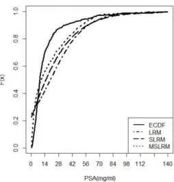
(see https://www.umass.edu/statdata/statdata/stat-logistic.html).The data is on 380 subjects of which 153 had tumor that penetrated the prostatic capsule. The variablecapsule denotes the status of the tumor, whether it is penetrated or not, which we consider as the dichotomous dependent variable(Y) andProstatic Spec-imen Antigen Value(PSA)in mg/ml as the explanatory (X) variable. These data set is also studied in (Hosmer and Lemeshow, 2000). These data are copyrighted by John Wiley and Sons Inc.

3

7

2

S

.

K

u

m

a

r

a

n

d

L

.

M

a

n Estimated values of the parameters with the corresponding PseudoR values and Information criteria values.

Distribution

Data set LRM(a, b) SLRM(λ, β, a, b) MSLRM(α, β, a, b) ˆ

α – – 12.134

ˆ

λ – 11.400 –

ˆ

β – 8.317 1.793

Data set 1 aˆ 0.154 11.774 0.006 ˆ

b 0.024 0.086 0.001

AIC 150.000 148.980 144.100 BIC 150.106 149.192 144.202 McFadden’sR2 _{0.040 0.073 0.105}

McFadden’s AdjR2 _{0.014 0.021 0.053}

Cox SnellR2 _{0.053 0.094 0.132}

Cragg-Uhler(Nagelkerke)R2 _{0.071 0.127 0.179}

ˆ

α – – 11.080

ˆ

λ – 34.100 –

ˆ

β – 13.238 9.170

Dataset 2 aˆ -1.114 5.044 -0.002 ˆ

b 0.057 0.488 0.0002 AIC 468.240 466.860 464.260 BIC 469.399 469.179 466.579 McFadden’sR2 _{0.094 0.104 0.109}

McFadden’s AdjR2 _{0.086 0.089 0.097}

Cox SnellR2 _{0.119 0.131 0.140}

Figure 2 – ECDF of the data set1 and fitted regression models - LRM, SLRM and MSLRM

TABLE 3

Calculated values of the test statistic Data set Hypothesis logL

_∧

Ω;y|x

logL

_∧∗

Ω ;y|x

Test statistic

H0:α= 0 -68.047 -73.001 9.908

Data set1

H0:α=−1 -68.047 -70.490 4.886

H0:α= 0 -228.130 -232.120 7.980 Data set2

H0:α=−1 -228.130 -230.430 4.600

6. Testing of hypothesis and Simulation

In this section we discuss certain test procedures for testing the significance of the additional parameterαof the MSLRM and carry out a brief simulation study for examining the performance of the maximum likelihood estimators. First we discuss the generalized likelihood ratio test procedure for testing the following hypothesis:

Test 1. H0: α = 0 against the alternative hypothesisH1: α 6= 0 Test 2. H0: α = −1 against the alternative hypothesis H1: α 6= −1. Here the test statistic is,

−2 log Λ = 2

logL

∧ Ω;y|x

−logL

∧∗ Ω ;y|x

(35)

where ∧

Ω is the maximum likelihood estimator of Ω = (α, β, a, b) with no restric-tion, and

∧∗

Ω is the maximum likelihood estimator of Ω whenα = 0 in case of Test 1 and α = −1 in case of Test 2. The test statistic −2 log Λ given in (35) is asymptotically distributed as χ2 with one degree of freedom (Rao, 1973). The computed values oflogL

_∧

Ω;y|x

, logL

_∧∗

Ω ;y|x

and test statistic in case of both

data sets are listed in Table 3.

Since the critical value at the significance level 0.05 and degree of freedom one is 3.84, the null hypothesis is rejected in both the case, which shows the appropriat-ness of the MSLRM to the data sets.

Next we conduct a simulation study for assessing the performance of the MLEs of the parameters of the MSLRM. We consider the following two sets of parame-ters.

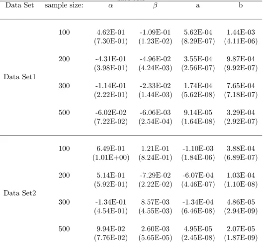
TABLE 4. Bias and Mean Square Error(M SE)within brackets of the simulated data sets

Data Set sample size: α β a b

100 4.62E-01 -1.09E-01 5.62E-04 1.44E-03 (7.30E-01) (1.23E-02) (8.29E-07) (4.11E-06)

200 -4.31E-01 -4.96E-02 3.55E-04 9.87E-04 (3.98E-01) (4.24E-03) (2.56E-07) (9.92E-07) Data Set1

300 -1.14E-01 -2.33E-02 1.74E-04 7.65E-04 (2.22E-01) (1.44E-03) (5.62E-08) (7.18E-07)

500 -6.02E-02 -6.06E-03 9.14E-05 3.29E-04 (7.22E-02) (2.54E-04) (1.64E-08) (2.92E-07)

100 6.49E-01 1.21E-01 -1.10E-03 3.88E-04 (1.01E+00) (8.24E-01) (1.84E-06) (6.89E-07)

200 5.14E-01 -7.29E-02 -6.07E-04 1.03E-04 (5.92E-01) (2.22E-02) (4.46E-07) (1.10E-08) Data Set2

300 -1.34E-01 8.57E-03 -1.34E-04 4.86E-05 (4.54E-01) (4.55E-03) (6.46E-08) (2.94E-09)

500 9.94E-02 2.60E-03 4.95E-05 2.07E-05 (7.76E-02) (5.65E-05) (2.45E-08) (1.87E-09)

The computed values of the bias and mean square error(MSE) corresponding to sample sizes 100, 200, 300 and 500 respectively are given in Table 4.

From the table it can be seen that both the absolute bias and MSEs in respect of each parameters of the MSLRM are in decreasing order as the sample size increases.

Acknowledgements

Appendix

A. Proofs of equation (9)

By definition, using the double series expansion for p.d.f, the c.d.f of theM SLD(α, β) takes the following form, forx < 0 .

F(x) = 2 α+ 2

  ∞ X k=0 −2 k _Zx −∞

e(1+k)xdx+α ∞ X j=0 ∞ X k=0 −1 j −2 k _Zx −∞

e(1+βj+k)xdx

 

= 2

α+ 2

  ∞ X k=0 −2 k

e(1+k)x (1 +k)+α

∞ X j=0 ∞ X k=0 −1 j −2 k

e(1+βj+k)x (1 +βj+k)



 (36)

In a similar way, the c.d.f of theM SLD(α, β) can be written as given below, for x ≥ 0.

F(x) = 1−

∞

Z

x

f(x)dx

= 1− 2

α+ 2

  ∞ X k=0 −2 k _Z∞ x

e−(1+k)x dx+α

∞ X j=0 ∞ X k=0 −1 j −2 k _Z∞ x

e−(1+β+βj+k)x dx

 

= 1− 2

α+ 2

  ∞ X k=0 −2 k

e−(1+k)x (1 +k) +α

∞ X j=0 ∞ X k=0 −1 j −2 k

e−(1+β+βj+k)x (1 +β+βj+k)



 (37)

Thus (36) and (37) gives (9).

References

A. A. Afifi, S. P. Azen (1979). Statistical Analysis: A Computer Oriented Approach. Academic Pres, New York.

A. Azzalini (1985). A class of distributions which includes the normal ones. Scandinavian Journal of Statistics, 12, pp. 171–178.

A. C. Cameron,F. A. Windmeijer(1996). R-squared measures for count data regression models with applications to health-care utilization. Journal of Business and Economic Statistics, 14, no. 2, pp. 209–220.

D. J. Finney(1952).Statistical methods in Biological Assay. Hafner Publications, NewYork.

P. R. Fisk (1961). The graduation of income distributions. Econometrica, 29, pp. 171–185.

D. Mcfadden(1973). Conditional logit analysis of qualitative choice behavior in zarembka,p. (ed.). InFrontiers in Econometrics, Academic Press, NewYork, pp. 105–142.

S. Nadarajah(2009).The skew logistic distribution. AStA. Adv. Stat. Anal, 93, pp. 187–203.

F. R. Oliver (1969). Another generalisation of the logistic growth function. Econometrica, 37, pp. 144–147.

R. L. Plackett (1959). The analysis of life test data. Technometrics, 1, pp. 9–19.

C. R. Rao (1973). Linear statistical inference and its applications. NewYork, Wiley.

Summary

Here we consider a modified form of the logistic regression model useful for situations where the dependent variable is dichotomous in nature and the explanatory variables exhibit asymmetric behaviour. Certain structrual properties of the modified skew logistic model is discussed and the proposed regression model has been fitted to some real life data sets by using the method of maximum likelihood estimation. Further, two data illustrations are given for highlighting the usefulness of the model in certain medical applications and a simulation study is conducted for assessing the performance of the estimators.