STATISTICAL METHODS FOR BAYESIAN CLINICAL TRIAL DESIGN
AND DNA METHYLATION DECONVOLUTION
Matthew A. Psioda
A dissertation submitted to the faculty at the University of North Carolina at Chapel Hill in partial fulfillment of the requirements for the degree of Doctor of Philosophy in the
Department of Biostatistics.
Chapel Hill 2016
Approved by:
Joseph Ibrahim
Wei Sun
Mengjie Chen
Yun Li
c
2016
Matthew A. Psioda
ABSTRACT
Matthew A. Psioda: Statistical Methods for Bayesian Clinical Trial Design and DNA Methylation Deconvolution
(Under the direction of Joseph Ibrahim and Wei Sun)
We consider the Bayesian clinical trial design problem in situations where a historical trial is
available to inform the design and analysis of a future trial. Currently the FDA requires that
all proposed designs exhibit reasonable type I error control. Traditionally, frequentist type I error
control has been required. This is currently the case in the Center for Drug Evaluation and Research
but no longer in the Center for Devices and Radiological Health. The requirement that a design
exhibit frequentist type I error control necessitates that all prior information be discarded. We
propose several Bayesian solutions that balance the need to control type I errors with the desire to
utilize high quality prior information.
For scenarios where the historical trial informs the parameter being tested, we propose Bayesian
versions of the type I error rate and power that are defined with respect to the posterior distribution
for the parameters given the historical data and conditional on the respective hypothesis being true.
We demonstrate that in designs that control the Bayesian type I error rate, meaningful amounts of
prior information can be borrowed but that the size of the new trial must be relatively large to justify
borrowing a large amount of historical information. We tailor our design methodology for survival
applications using proportional hazards and cure rate models. We also develop Bayesian adaptive
designs for large cardiovascular outcomes trials (CVOTs) which incorporate control information
from a historical CVOT conducted in a similar patient population. We propose an all-or-nothing
adaptive design utilizing the power prior as well as a dynamic borrowing adaptive design utilizing
a novel extension of the joint power prior.
Separately, we present a statistical deconvolution method for DNA methylation data from
heterogeneous tissue samples and another set of reference tissue samples. Unlike other methylation
deconvolution methods, our method allows one to estimate the heterogeneous tissue composition
and provides improved estimates of cell type-specific methylation levels through the process of
de-convolution. We demonstrate our method using data from DNA mixture tissues and simulation
ACKNOWLEDGMENTS
I would first like to thank the three people whose love and support has been indispensable to
me throughout my life. To my wife, Ashley, I would like to say thank you for being there for me
throughout this journey. There were many challenging times and I surely would have fallen short
of my goals without your love and support. You are my rock and my best friend. To my mother,
Linda, I would like to say thank you for listening, advising, comforting, and supporting me. I hope
my reaching this point make you as proud of me as I am proud to be your son. To my father, Terry,
I would like to say thank you for your unfailing example and for teaching me the value of honest
hard work.
I would like to thank my advisors, Dr. Joseph Ibrahim and Dr. Wei Sun. I am truly grateful for
all of the time they have shared with me over the past five years and for all of the doors they have
helped me open. I would like to thank Dr. Mat Soukup for the mentorship given to me during my
fellowship with the Food and Drug Administration. I would also like to thank Dr. Mengjie Chen,
Dr. Kathleen Dorsey, and Dr. Yun Li for serving on my doctoral committee. I would like to thank
the National Cancer Institute for supporting three years of my research through the Biostatistics
for Research in Genomics and Cancer Training Grant (NCI grant 5T32CA106209-07) and the Food
and Drug Administration for supporting one year.
I have made many good friends in the past five years. The closest of which are James Xenakis
and Elizabeth Rowley. I would like to thank them both for their companionship, their help in all
TABLE OF CONTENTS
LIST OF TABLES . . . ix
LIST OF FIGURES . . . x
CHAPTER 1: INTRODUCTION. . . 1
CHAPTER 2: LITERATURE REVIEW. . . 3
2.1 Bayesian Clinical Trial Design . . . 3
2.2 Bayesian Analysis of Proportional Hazards and Cure Rate Models . . . 9
2.3 DNA Methylation Deconvolution. . . 11
CHAPTER 3: BAYESIAN DESIGN OF A SURVIVAL TRIAL UNDER A PROPORTIONAL HAZARDS ASSUMPTION USING HISTORICAL DATA. . . 17
3.1 Introduction . . . 17
3.2 The Piecewise Constant Hazard Proportional Hazards Model . . . 20
3.3 The Posterior Distribution under the Basic Power Prior . . . 21
3.3.1 A Connection with the Weighted Cox Partial Likelihood . . . 23
3.4 Simulation-Based Bayesian Design of a Superiority Study . . . 24
3.4.1 Definition of the Bayesian Type I Error Rate and Power . . . 25
3.4.2 Default Sampling Priors . . . 27
3.4.3 Modifications to the Default Sampling Priors . . . 29
3.4.4 Estimation of the Bayesian Type I Error Rate and Power . . . 30
3.4.5 Efficient Computation of Posterior Quantities . . . 31
3.5 Application: Design of a Superiority Study . . . 32
3.6 Discussion . . . 38
4.1 Introduction . . . 40
4.2 The Promotion Time Cure Rate Model . . . 43
4.3 The Basic Power Prior and the Posterior Distribution . . . 47
4.4 Simulation-Based Bayesian Design of a Superiority Trial . . . 49
4.4.1 Definition of the Bayesian Type I Error Rate and Power . . . 50
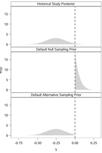
4.4.2 Default Sampling Priors . . . 51
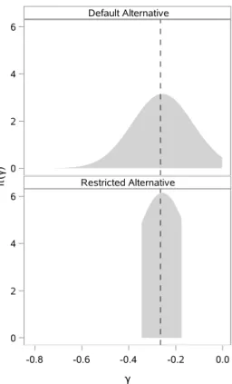
4.4.3 Alternatives to the Default Sampling Priors . . . 53
4.4.4 Estimation of the Bayesian Type I Error Rate and Power . . . 55
4.5 Bayesian Design of a Superiority Trial in High-Risk Melanoma . . . 56
4.6 Discussion . . . 64
CHAPTER 5: BAYESIAN DESIGN OF A CARDIOVASCULAR OUTCOMES TRIAL. . . 66
5.1 Introduction . . . 66
5.2 Practical Design Considerations . . . 69
5.3 The Piecewise Constant Hazard Proportional Hazards Model . . . 72
5.4 Adaptive Design Strategies . . . 73
5.4.1 All-or-Nothing Adaptive Design . . . 74
5.4.2 Dynamic Borrowing Adaptive Design . . . 76
5.5 The Simulation-Based Design Strategy . . . 79
5.5.1 Stoppage Criteria for All-or-Nothing Adaptive Designs . . . 81
5.5.2 Stoppage Criteria for Dynamic Borrowing Adaptive Designs . . . 82
5.6 Designing a CVOT to Borrow from the SAVOR Trial . . . 82
5.7 Discussion . . . 87
CHAPTER 6: DNA METHYLATION DECONVOLUTION USING BISULFITE SEQUENCING DATA . . . 89
6.1 Introduction . . . 89
6.2 A Simple Deconvolution Model . . . 91
6.2.2 On Overdispersion in the Cell Type-Specific Methylation Model . . . 94
6.3 Estimation of Tissue Composition in DNA Mixture Experiments . . . 95
6.4 Estimation of Tissue Composition and Cell Type-Specific Methylation in Simulation Studies . . . 98
6.5 Discussion . . . 102
CHAPTER 7: FUTURE WORK. . . 104
7.1 Bayesian Clinical Trial Design . . . 104
7.2 DNA Methylation Deconvolution. . . 105
APPENDIX A: CHAPTER 3 SUPPLEMENTAL MATERIALS. . . 106
A.1 Type I Error Control with Informative Priors . . . 106
A.2 Bayesian Design with Unshared Parameters . . . 111
A.3 A Simulation Study Comparing Inference Based on the PWC-PH model with Inference Based on the Weighted Cox Partial Likelihood . . . 113
A.4 A Simulation Study Comparing Exact Bayesian Inference Through MCMC with the Laplace Approximation . . . 115
A.4.1 High Throughput Model Fitting with MCMC . . . 115
A.4.2 A Comparison of MCMC Analysis Results with Results based on the Laplace Approximation . . . 116
APPENDIX B: CHAPTER 4 SUPPLEMENTAL MATERIALS. . . 118
B.1 A Simulation Study Comparing Bayesian Inference using MCMC with the Weighted Maximum Likelihood Approximation . . . 118
APPENDIX C: CHAPTER 5 SUPPLEMENTAL MATERIALS. . . 120
C.1 Integral Computation for the Restricted Maximal Borrowing Power Prior . . . 120
LIST OF TABLES
3.1 Summary survival data for selected E1684 subjects . . . 33
3.2 Posterior summaries for historical trial . . . 34
3.3 Posterior summaries for default sampling priors . . . 34
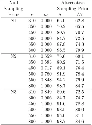
3.4 Bayesian power estimates under various sampling priors . . . 37
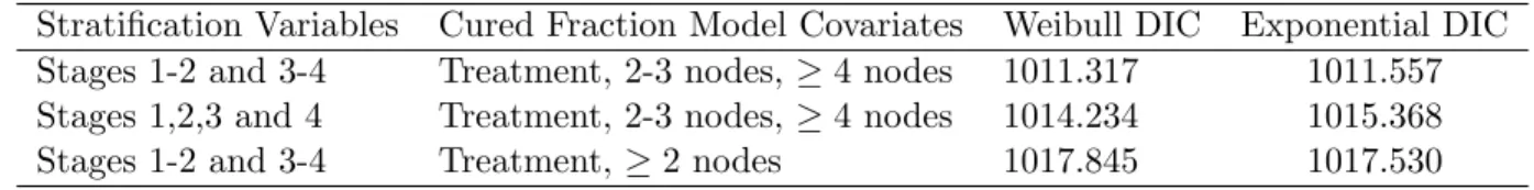
4.1 DIC for six best candidate design models . . . 58
4.2 Posterior summaries for the historical trial and default sampling priors . . . 58
4.3 Power estimates for select sample sizes . . . 63
5.1 Posterior summaries for SAVOR trial . . . 84
5.2 Optimal adaptive designs . . . 86
6.1 DNA Mixture tissue composition fraction estimate quality . . . 98
6.2 Tissue composition fraction estimate quality . . . 101
6.3 Cell type-specific methylation estimate quality . . . 101
A.1 Summary of inference agreement using the PWC-PH model and the weighted Cox partial likelihood . . . 114
A.2 Summary of inference agreement using MCMC and the Laplace ap-proximation . . . 117
LIST OF FIGURES
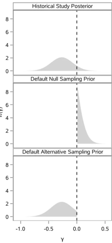
3.1 π(γ|D0) and corresponding default marginal sampling priors . . . 28
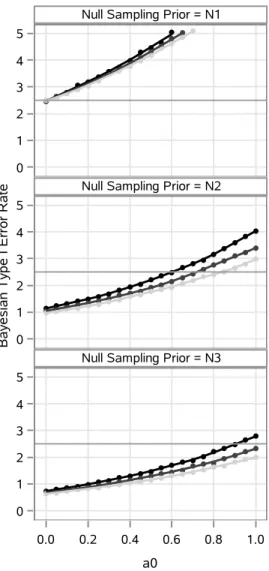
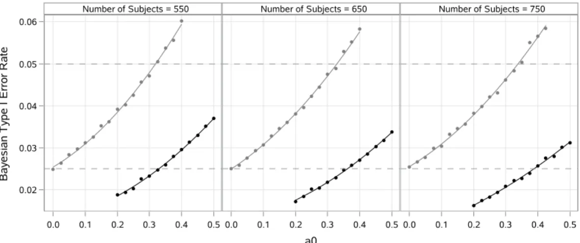
3.2 Loess curves and point estimates of the Bayesian type I error rate . . . 36
4.1 π(γ|D0) and corresponding default marginal sampling priors . . . 52
4.2 Alternative marginal sampling priors for γ. . . 55
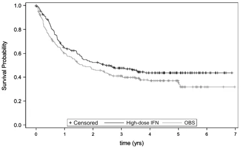
4.3 Kaplan-Meier curves for the high-dose INF and OBS groups . . . 57
4.4 Regression curves and point estimates of the Bayesian type I error rate . . . 60
4.5 Regression curves and point estimates for a0 as a function of sample size for designs that control the Bayesian type I error rate . . . 61
4.6 Regression curves and point estimates for Bayesian power as a function of sample size when the value of a0 is chosen to control the Bayesian type I error rate . . . 62
6.1 Estimated cell type composition in 18 DNA mixture tissues. . . 97
CHAPTER 1: INTRODUCTION
In this dissertation we present research on two important but otherwise unrelated topics. The
first topic, which is treated with the most depth, is the problem of Bayesian clinical trial design in
situations where a previously completed clinical trial (i.e. a historical trial) is available to inform
the design and analysis of a future trial. The traditional frequentist approach to clinical trial design
requires that the type I error rate be controlled for every possible null value of the parameters.
However, such control is impossible if one wishes to incorporate any subjective prior information.
We propose several Bayesian design solutions that balance the need to control type I errors with
the desire to utilize high quality prior information for the purpose of decreasing the size or duration
of a future trial.
In Chapters 3 and 4 we propose and apply Bayesian versions of the type I error rate and
sta-tistical power in the design of superiority trials for time-to-event data. These Bayesian operational
characteristics are defined with respect to the posterior distribution for the parameters given the
historical trial data and conditional on the respective hypothesis being true. Chapter 3 focuses
on design (i.e. sample size determination) for time-to-event trials where a proportional hazards
assumption is tenable. Chapter 4 focuses on designs for time-to-event trials where a fraction of the
studied population is “cured” (i.e. immune to having the event).
In Chapter 5 we consider the design of large cardiovascular outcomes trials (CVOTs) utilizing
data from control subjects from a previously completed CVOT (i.e. a historical CVOT). Borrowing
information only through the control arm presents unique challenges. The benefit of randomization
in the new trial is essentially lost and it becomes important to adjust for prognostic factors to help
ensure subjects in the two trials are exchangeable. We develop two Bayesian adaptive designs to
address a potential lack of exchangeability: an all-or-nothing borrowing approach using the basic
power prior (Ibrahim and Chen, 2000) and an adaptive borrowing approach using a novel restricted
2000).
In Chapter 6 we switch our focus to the second topic: statistical deconvolution of DNA
methy-lation levels. In this chapter we present a deconvolution method for DNA methymethy-lation data from
bisulfite sequencing experiments. We propose a joint model for methylation data from a set of
heterogeneous tissue samples and a set of reference tissue samples. Unlike other deconvolution
methods, our methods allows one to estimate the heterogeneous tissue composition and provides
improved estimates of cell type-specific methylation levels through the process of deconvolution.
Our method allows one to assess methylation at the cell type level whereas commonly used
reference-free methods do not. We demonstrate our method using real data from DNA mixture experiments
CHAPTER 2: LITERATURE REVIEW
2.1 Bayesian Clinical Trial Design
There is a growing demand for principled ways to incorporate knowledge from previously
com-pleted clinical trials in the design and analysis of future trials. Regulatory authorities, such as the
Food and Drug Administration (FDA), are increasingly embracing Bayesian methodology for this
purpose. For example, in 2010 the FDA issued guidance on using Bayesian methods in medical
device clinical trials (Food and Drug Administration, 2010). Recently, additional guidance has
been issued that discusses using Bayesian methods to extrapolate information from adult trials
to pediatric populations (Food and Drug Administration, 2016). At the Center for Devices and
Radiological Health, companies are encouraged to take advantage of good prior information on the
safety and effectiveness of their investigational devices through formal Bayesian analysis (Pennello
and Thompson, 2007). The FDA sees great promise in using Bayesian methods for incorporation
of prior information as well as for conducting adaptive trials (Campbell, 2011).
There is an extensive literature on Bayesian sample size determination methods. Details in
book format can be found in Spiegelhalter et al. (2004). Somewhat outdated reviews are given by
Adcock (1997) and Pezeshk (2003). Brief summaries of more recent work focusing on traditional
Bayesian operating characteristics are as follows:
Wang and Gelfand (2002) formalized a general Bayesian framework that can be used to calculate
the required sample size such that certain characteristics of the posterior meet a specified criteria
based on an assumed sampling model for the data, sampling prior for the parameters, and fitting
prior for the analysis. An example criterion is the average posterior variance criterion (APVC).
For this criterion, one seeks a sample sizensuch that Evar h(θ)yn
≤for some chosen >0,
expectation is with respect to the prior predictive distribution for the data defined by the sampling
model for the data and sampling prior for the parameters. The authors present two sample size
determination examples. One is based on a survival model with censoring and the other is based on
a logistic regression model. This simulation-based framework has been widely adopted for Bayesian
sample size determination.
Pham-Gia and Turkkan (2003) present a computationally-intensive method to calculate the
exact sample size required so that the expected length of the highest posterior density (HPD)
interval for the difference in two binomial proportions is sufficiently small. M’Lan et al. (2008)
investigate binomial sample size determination using generalized versions of the average length
and average coverage criteria, median length and median coverage criteria, and the worst outcome
criterion (Joseph et al., 1995). They compare sample sizes derived from highest posterior density
intervals and equal-tailed credible intervals. In some cases, they develop closed-form sample size
formulas.
De Santis (2004) considers the problem of choosing the sample size for testing hypotheses using
Bayes factors. The predictive criterion proposed for determining the sample size is maximizing the
probability of obtaining substantial evidence in favor of the true hypotheses (or, equivalently
min-imizing the probabilities of having either misleading or weak evidence). The method is developed
for the normally distributed data and applied to the design of a bladder cancer clinical trial.
Inoue et al. (2005) explore parallels between Bayesian and frequentist methods for determining
sample size. The authors provide a simple but general framework for investigating the
relation-ship between the two approaches, based on identifying mappings to connect the Bayesian and
frequentist inputs necessary to obtain the same sample size. They highlight a somewhat
surpris-ing “approximate functional correspondence” between power-based and information-based optimal
sample sizes.
De Santis (2006) presents a robust Bayesian approach to the sample size determination problem
based on the lower bound, upper bound, and range of posterior quantities of interest. These
characteristics (e.g. the lower bound) are obtained by varying the prior over a class of distributions.
will observe a small value of the range and either a sufficiently large lower bound or a sufficiently
small upper bound for the posterior quantity of interest.
Clarke and Yuan (2006) give asymptotic expressions for the expected value (under a fixed
pa-rameter) of certain types of functionals of the posterior density. They obtain simple inequalities
which can be solved to give minimal sample sizes needed for various estimation goals. The
au-thors verify that the asymptotic bounds give good approximations to the expected values of the
functionals they approximate.
De Santis (2007) presents a general sample size determination method with a goal of choosing
the minimal sample size that guarantees probabilistic control on the performance of quantities that
are derived from the posterior distribution and used for inference. The author illustrates how the
class of power priors (Ibrahim and Chen, 2000) can be fruitfully employed to deal with lack of
homogeneity between historical data and observations of the upcoming experiment. The authors
discuss the need for discounting prior information and evaluating the effect of heterogeneity on the
optimal sample size. Some of the most popular Bayesian operational characteristics are reviewed
and their use is illustrated in several examples.
Brutti et al. (2008) consider determination of a sample size that guarantees a large posterior
probability that an unknown parameter of interest (e.g. a treatment effect) is greater than a chosen
threshold. The authors argue that a straightforward sample size criterion is to select the minimal
number of observations so that the predictive probability of a successful trial is sufficiently large.
In the paper the authors address sensitivity to prior assumptions by proposing a robust version
of the sample size criterion. Specically, instead of using a single prior distribution, the authors
consider a class of plausible priors for the parameter of interest. Robust sample sizes are then
selected by looking at the predictive distribution of the lower bound of the posterior probability
that the unknown parameter is greater than a chosen threshold. The authors consider classes of
-contamination priors (Berger and Berliner, 1986) for the flexibility and mathematical tractability.
Most of the aforementioned works have focused on computing sample size based on “traditional”
Bayesian operating characteristics (i.e. the APVC). As noted above, regulatory bodies such as the
is natural to plan a Bayesian clinical trial where the prior is calibrated to ensure adequate type
I error control and power. The idea that these operating characteristics should be considered for
Bayesian clinical trial designs is not new (Rubin et al., 1984; Box, 1980). A variety of authors have
approached Bayesian sample size determination from the perspective of statistical power and type
I error rates with some attempting to incorporate subjective prior information in the design. Brief
summaries of selected works are as follows:
Spiegelhalter and Freedman (1986) develop sample size determination method which takes into
account prior clinical opinion about the treatment difference. This method adopts the point of
clinical equivalence (determined by interviewing the study participants) as the null hypothesis.
Decision rules at the end of the study are based on whether the interval estimate of the treatment
difference includes the null hypothesis. The prior distribution is used to predict the probabilities
of making the decisions to select one of the two treatments or to reserve final judgment. The
authors advocate that the sample size be chosen to control the predicted probability of reserving
final judgment. An example is presented using normally distributed data from a cancer clinical
trial.
Brown et al. (1987) present a sample size determination method that uses the results of a
historical study to predict the outcome of a subsequent trial in a setting where the response is binary.
The author’s method can be easily generalized to other two-sample cases for which power can be
calculated in closed-form (e.g. exponential survival), and to one-sample cases such as demonstrating
a minimal response rate. Bayesian methods are used to obtain a posterior distribution based on
an analysis of the historical study and this posterior is used as the “state of knowledge” for the
parameters of interest. The probability that the future study will demonstrate treatment superiority
is obtained by using the posterior distribution to compute the average power over the parameter
space.
Weiss (1997) presents an approach to sample size determination that aims to make it a priori
probable that the Bayes factor will be greater than a given cut-off of prespecified size. Similar
to Brown et al. (1987), the approach permits the propagation of uncertainty in quantities which
rates either conditionally (i.e. conditional on the effect size being larger than a certain value) or
unconditionally (based on the prior distribution for the effect size). The approach is illustrated for
a one-sided and for a two-sided alternative hypothesis for continuous data with a normal prior.
Chen et al. (2011) develop a sample size determination method specifically for the design of
non-inferiority clinical trials using subject-level historical control data. The authors compare a
hierarchical modeling approach for information borrowing (which necessitates multiple historical
studies) with the power prior approach of Ibrahim and Chen (2000). The authors consider use
of the basic power prior which fixes the amount of information borrowed a priori as well as the
normalized power prior (Duan, 2005; Duan et al., 2006) which attempts to dynamically adjust the
amount of information borrowed from the historical study based on the level of agreement between
the two data sets. We note that the historical studies only provide information on the control group
in the case study and the type I error and power are computed under the implicit assumption that
the generative model for the new study data is consistent with the historical data. Hence the type I
error control demonstrated by the method is not as stringent as traditional frequentist type I error
control. The normalized power prior is a special case of the joint power prior proposed by Ibrahim
and Chen (2000) and it was developed to address some shortcomings of the joint power prior that
were described in Duan (2005).
Hobbs et al. (2011) propose the commensurate power prior which is another extension of the
normalized power prior (Duan, 2005; Duan et al., 2006). The commensurate power prior is quite
different from the normalized power prior in that it does not assume a common parameter in the
models for the historical and new study. Instead the new study parameter is assumed to be normally
distributed about the historical study parameter. The precision parameter in the normal component
of the commensurate power prior is called the commensurability parameter and this parameter is
incorporated into the prior for the parameter that controls the amount of information borrowed (i.e.
the power on the historical study likelihood). The authors compare the frequentist performance
of several informative prior choices using simulations and present an example using a colon cancer
trial that illustrates the adaptive borrowing approach in the case of a linear model. In general the
method does not lead to frequentist type I error control. However, the authors further compare
normalized power prior) where all methods control the type I error rate at the nominal level. The
power function with the largest area under the curve was based on the author’s commensurate
power prior. One draw back of the authors approach is that is requires normally distributed data
to apply without approximation. Hobbs et al. (2012) propose extensions to the commensurate
power prior and evaluate the frequentist and Bayesian properties using general and generalized
linear mixed regression models. The authors provide an example analysis of a colon cancer trial
comparing time-to-disease progression using a Weibull regression model. Use of the commensurate
power prior (as well as the normalized power prior and joint power prior) are closely related to
meta-analysis. Determining a sample size for a future study using these meta-analytic priors is
challenging due to the computational burden of fitting models with them. A complete review of
the basic power prior and its generalizations can be found in Ibrahim et al. (2015).
Ibrahim et al. (2012b) develop a Bayesian meta-analysis framework using survival regression
models to assess whether the size of a clinical development program is adequate to evaluate a
partic-ular safety endpoint. Their sample size determination methodology for meta-analysis clinical trial
design focuses on controlling the type I error rate and providing adequate statistical power. Using
the partial borrowing power prior (i.e. the basic power prior where not all parameters are shared
between the new and historical study), the authors incorporate the historical survival meta-data
into the statistical design. The authors develop a simulation-based algorithm for estimating relevant
operational characteristics of the Bayesian meta-analysis trial design. The proposed methodology
is applied to the design of a phase 2/3 development program including a non-inferiority clinical trial
for CV risk assessment in type II diabetes mellitus (T2DM). In Chen et al. (2014a) this
methodol-ogy is extended to a group sequential clinical trial design framework. In both papers the authors
show that minimal information can be borrowed without inflating the type I error rate (e.g. that
one can borrow ≤ 2% of the available information). The version of type I error rate that the
authors attempt to control is essentially the same as in Chen et al. (2011) with the only difference
being that information is being borrowed on the parameter being tested. This key difference makes
information borrowing essentially impossible.
Chen et al. (2014b) propose a Bayesian approach for the design of superiority clinical trials
completed trial are incorporated into the design via the partial borrowing power prior. The authors
develop a simulation-based algorithm for computing various design quantities such as the type I
error rate and power. Similar to Ibrahim et al. (2012b) and Chen et al. (2014a), the results
demonstrate that little information can be borrowed if the design is required to control type I error
in a traditional sense.
2.2 Bayesian Analysis of Proportional Hazards and Cure Rate Models
Bayesian analysis of proportional hazards and cure rate models has been considered by many
authors. We briefly review the relevant literature in this section. A definitive text on Bayesian
survival analysis was provided by Ibrahim et al. (2001b). This text includes extensive discussion
on Bayesian analysis of proportional hazards models as well as cure rate models.
Bayesian analysis of the Cox partial likelihood (Cox, 1975) dates back to the work of Kalbfleisch
(1978) who was the first to give a fully Bayesian justification. A definitive work on Bayesian
justifications of the partial likelihood was given by Sinha et al. (2003). Therein the authors establish
new (both naive and formal) Bayesian justifications for the Cox partial likelihood and its various
modifications. The authors consider cases with time-dependent covariates, time-varying regression
parameters, continuous time survival data, and grouped survival data. In addition, the authors
present a Bayesian justification of a modified partial likelihood for handling ties.
Ibrahim and Chen (1998) propose a class of informative prior distributions for a proportional
hazards model. A novel construction of the prior is developed based on the notion of the availability
of historical data and using the power prior. This work discussed using the power prior several years
before the work of Ibrahim and Chen (2000), wherein the power prior was formalized. The authors
took a semi-parametric approach for modeling the baseline hazard which has become standard for
Bayesian proportional hazards models. They also developed an efficient Gibbs sampling framework
for model fitting.
Cure rate models date back to Berkson and Gage (1952) where the mixture cure rate model
was formalized. The authors develop a simple mixture model for survival data where an unknown
exponential survival distribution. The class ofpromotion time cure rate models are an important
subclass of mixture cure rate models. The promotion time cure rate model was originally proposed
by Yakovlev et al. (1993). These models have a natural biological motivation based on a latent
competing risk framework where metastasis competent tumor cells (that survive treatment) define
the competing risks.
Bayesian analysis of promotion time cure rate models was considered first by Chen et al. (1999).
The authors provide a thorough discussion of the natural motivation and interpretation of the
model and derive several novel properties of it. In particular, the authors show that the model has
a proportional hazards structure on the marginal subhazard when the cured fraction is modeled
as a function of covariates. They also establish a mathematical connection with the standard
mixture cure rate model. They discuss prior elicitation in some detail and propose classes of
non-informative and informative prior distributions (the power prior being among them). Several
theoretical properties of the proposed priors and resulting posteriors are derived.
Ibrahim et al. (2001a) extend the Bayesian version of the promotion time cure rate model given
in Chen et al. (1999). Specifically, the authors propose a semi-parametric cure rate model with
a smoothing parameter that controls the degree of parametricity in the right tail of the survival
distribution. The authors argue that such a parameter is important for these models and can
influence posterior estimates. Several novel properties of the proposed model are derived and a
class of informative priors based on historical data is proposed (i.e. the power prior). A case study
involving a melanoma clinical trial is discussed in detail to demonstrate the proposed methodology.
Chen et al. (2002a) provide an interesting comparison of several Bayesian models for
time-to-event data. They consider a piecewise exponential baseline hazard proportional hazards model, a
fully parametric cure rate model, and a semi-parametric cure rate model. For each model, they
derive the likelihood function and examine some of its properties for carrying out Bayesian inference
with non-informative priors. They also examine model identifiably issues and give conditions which
guarantee identifiably. The authors compare the performance of the models based on the conditional
predictive ordinate (CPO) which is defined using the posterior predictive distribution for each data
study using the E1690 clinical trial (Kirkwood et al., 2000).
Ibrahim et al. (2012a) consider a joint analysis of the E1684 clinical trial (Kirkwood et al.,
1996) and the E1690 clinical trial (Kirkwood et al., 2000) using cure rate models and the power
prior. This was an interesting application of Bayesian methods to synthesize information from two
clinical trials but it did not address how to design a future trial given information from a previously
completed clinical trial.
2.3 DNA Methylation Deconvolution
The concept of DNA methylation deconvolution arises in two types of studies. In studies aimed
at identifying associations between DNA methylation and phenotypes of interest (e.g. comparing
diseased cases and healthy controls), researchers generally measure methylation levels using
het-erogeneous tissue samples, such as blood, which can be collected easily. The tissue samples are
heterogeneous in the sense that they are comprised of several (possibly many) functionally distinct
cell types with each having a potentially distinct DNA methylation signature that may or may not
be associated with the disease phenotype. For example, blood contains many different types of
white blood cells, including neutrophils, basophils, eosinophils, lymphocytes, and monocytes. In
addition to white blood cells, organs such as the liver can contribute significantly to the circulating
pool of DNA in blood (Lo et al., 1998). Presumably, each cell type represented in a heterogeneous
tissue contributes DNA for the methylation measurement in accordance with its relative
abun-dance in the tissue sample. If the cell types comprising a set of heterogeneous tissue samples have
functionally different methylation signatures, as they do in blood (Reinius et al., 2012; Houseman
et al., 2012), it is critically important to control for cell type composition in analyses that attempt
to establish associations between tissue-level methylation and phenotypes of interest. This fact is
increasingly appreciated and it has been argued that many purported associations between age and
DNA methylation can be attributed to tissue composition bias that was poorly addressed in the
analysis (Jaffe and Irizarry, 2014).
In studies aimed at identifying associations between tissue composition and phenotypes of
In this setting, the DNA methylation levels of the constituent cell types are not of direct interest.
Rather, the cell type-specific DNA methylation levels simply offer a means to estimate the
het-erogeneous tissue’s composition. For example, Sun et al. (2015) performed a tissue composition
study in hepatocellular carcinoma (HCC) and observed increased levels of liver DNA in plasma
from cancer patients compared to healthy controls. Tissue composition studies require estimates
for the DNA methylation levels of the constituent cell types. These estimates typically comes from
reference tissue samples that are comprised predominately of one cell type though they are
gener-ally not perfectly homogeneous (Reinius et al. (2012), supplemental table 2). The reference tissues
are constructed through a procedure such as fluorescence activated cell sorting (FACS), which can
be laborious. As a result, reference tissues often have few replicates (biological or technical). In
the case of bisulfite sequencing data, there are often no replicates of any kind.
Broadly speaking, one may define DNA methylation deconvolution as the process of estimating
cell type-specific methylation levels and/or heterogeneous tissue composition using DNA
methyla-tion levels measured from heterogeneous tissue samples. The statistical approaches developed for
these studies generally fall into two classes: reference-based and reference-free methods.
Reference-based methods can be utilized for both types of studies described above whereas reference-free
methods are generally only useful for studies attempting to associate tissue-level methylation with
phenotypes of interest.
Reference-based methods use a set of reference samples from homogeneous cell type tissues
corresponding to the cell types thought to be in the heterogeneous tissues. The reference
tis-sue samples serve as the basis for deconvolution. Houseman et al. (2012) proposed the most
widely used method to estimate cell-type composition in blood. The method was designed for the
InfiniumRHumanMethylation27 BeadChip and a set of reference samples was published along with the statistical methodology. In the publication, the authors identified a subset of probes that were
informative for the white blood cell types and these probes were used in the deconvolution process.
Jaffe and Irizarry (2014) extended the method by augmenting the selected probe set based on the
InfiniumRHumanMethylation450 BeadChip, which is newer and more popular. The Houseman reference-based method is similar in spirit to a regression calibration method and is based on a
tissue methylation levels is
Y0h =β0w0h+0h
whereY0h is anm×1 vector of methylation values corresponding to homogeneous cell type tissue
sample h, w0h is a d0 ×1 ANOVA type covariate vector that identifies the cell type to which a
measurement corresponds,β0 is am×d0 matrix of average methylation values for thed0 cell types
at the m loci, and 0h is a vector of errors. The model for the heterogeneous tissue methylation
levels is
Y1i =β1z1i+1i
whereY1i is a m×1 vector of methylation values corresponding to heterogeneous tissue sample i,
z1i is ad1×1 covariate vector, β1 is am×d1 matrix, and1i is a vector of errors. The surrogacy
model is given by
β1 =1mγ0T +β0Γ+U
where Γ is a d0 ×d1 matrix that summarizes the associations between the rows of β0 and β1,γ0
is a d1 ×1 vector and U is a matrix of errors. The author shows that, under some conditions,
one can estimate the cell type compositions of the heterogeneous tissues from this model. The key
assumption is that E [Y1i|z1i] can be written as
E [Y1i|z1i =z] = ξ(z)+ d0 X
k=1
b0,kω(z)k
where β0 = (b0,1, . . . ,b0,d0), ω
(z)
k is the cell type k mixture fraction in the tissue, and ξ(z) is an
m×1 vector that is orthogonal to the column space ofβ0. The authors show that the orthogonality
assumption can be verified to some degree through sensitivity analysis but that bias results when it
does not hold. As noted above, the extension of this method by Jaffe and Irizarry (2014) was simply
true average cell type methylation levels, it does not produce refined estimates of those methylation
levels by incorporating information from the heterogeneous tissues.
In a study of methylation levels in rheumatoid arthritis patients, Liu et al. (2013) attempted
to adjust for cell type composition using estimates from the Houseman referenced-based method
in a simple linear regression model. Jaffe and Irizarry (2014) demonstrated this may be a poor
approach. Jaffe and Irizarry (2014) also consider a surrogate variables approach, named RUV
(Gagnon-Bartsch and Speed, 2012), that out performed the naive method of adjustment used by
Liu et al. (2013). Application of the RUV method still resulted in significant confounding compared
to a gold standard approach based on FACS. The RUV approach attempts to remove unwanted
variation (hence the name) based on a set of negative control probes. Note that the RUV approach
was not designed to solve the deconvolution problem and so the poor performance is not surprising.
Similar approaches to that used by Liu et al. (2013) have been proposed by others. For example,
Monta˜no et al. (2013) and Guintivano et al. (2013) propose methods specifically for brain tissue
that use data from the CHARM array (Irizarry et al., 2008).
The second class of statistical methods are reference-free. This class of methods has the same
goal as the reference-based methods used by Liu et al. (2013), Monta˜no et al. (2013), and
Guinti-vano et al. (2013) in that they attempt to provide a valid comparison of tissue-level methylation by
adjusting for cell type composition. However, as suggested by their name, reference-free methods
do so without requiring reference samples. Houseman et al. (2014) employ a singular value
decom-position (SVD) to separate cell-comdecom-position effects from the effect of interest. Zou et al. (2014) use
a similar approach but the role of dependent and independent variables are reversed. The potential
utility of reference-free methods is obvious. They do not require the potentially burdensome step
of obtaining reference tissue samples. However, reference-free methods cannot provide information
about cell type-specific methylation levels which is ultimately the level of granularity that is of
greatest biological importance. Moreover, the reference-free methods are designed to detect
so-called direct effects which may not fit the biological process under study. Houseman et al. (2014),
propose the model
Ω = XΓ+Ξ
where Y is an m×n matrix of methylation values, B is an m×p matrix of direct epigenetic
effects, Γ is a p×k coefficient matrix representing cell-proportion effects, X is a n×p matrix of
covariates, Mis an m×k matrix of cell type-specific mean methylation values (falling between 0
and 1),Ωis ann×kmatrix of of subject-specific cell proportions, Eis an m×nmatrix of errors,
and Ξis an n×k matrix of errors. The authors state that in adjusted epigenome-wide association
studies (EWAS), Bis of direct interest. These direct affects can be interpreted as covariate effects
that influence methylation levels in all cell types in the heterogeneous tissue equally and hence
are not mediated by cell composition. However, since the covariates may also be associated with
compositional differences, it is important to correct for tissue composition in the analysis. While
such direct affects may indeed exist, we find it more reasonable to posit that covariates (e.g. disease
phenotype) may influence the methylation level for one or more cell types in the tissue. Such cell
type-specific methylation effects are harder to study but may be more biologically meaningful. The
reference-free method proposed by Houseman et al. (2014) was used by Charlton et al. (2014) in
the study of Wilms tumors. Houseman et al. (2015) provide an review-like discussion of DNA
methylation deconvolution using the InfiniumRBeadChip data.
Recently deconvolution using bisulfite sequencing (BS-seq) data has been studied. This type
of data presents unique challenges. For methylation data collected using InfiniumRBeadChip technology, multiple replicates for reference tissues are typically available (e.g. data from Houseman
et al. (2012) and Reinius et al. (2012)). However, for BS-seq data, reference tissues generally do not
have replication making the method of Houseman et al. (2012) impossible to apply with adaptation.
Sun et al. (2015) use a quadratic programming approach (Van den Meersche et al., 2009) to solve
a simultaneous system of equations constructed using methylation estimates from heterogeneous
tissue samples using 14 reference tissue samples: liver, lungs, esophagus, heart, pancreas, colon,
small intestines, adipose tissues, adrenal glands, brain, T cells, B cells, neutrophils, and placenta.
The majority of these data were collected as a part of the NIH Roadmap Epigenomics project
(Bernstein et al., 2010) and do not have replicates (biological or technical) although some of the
identified a set of 5,820 genomic regions (500bp in length) that were informative of the 14 reference
tissue types. For each region the methylation level in each of the samples was estimated as the
percentage of all CpGs that were methylated. Then, for heterogeneous tissue sample s= 1, ..., S,
the following linear system was solved
Ys = Mρs
where Ys is a m×1 vector of estimated methylation levels in heterogeneous tissue sample s at
them genomic regions, Mis the m×kmatrix of estimated methylation levels for the k reference
samples considered in a given deconvolution problem (k was generally 5-6, not 14) andρs was the
unknownk×1 vector of tissue composition fractions that satisfied the constraints that 0≤ρs,j ≤1
forj = 1, ..., kandPk
j=1ρs,j = 1. The authors first demonstrated their method was able to recover
the composition fractions of DNA mixture tissues. Then, the authors demonstrated their method
on a real data set comprised of plasma samples from 15 pregnant women (five from each trimester)
and validated their ability to estimates the placental composition in the mother’s blood plasma
using paternally inherited fetal SNP alleles that were not possessed by the mother.
Ziller et al. (2013) use a similar quadratic programming algorithm to deconvolve in silico
mix-tures of HUES64 and hippocampus whole genome bisulfite sequencing (WGBS) libraries (i.e.
het-erogeneous tissues constructed by combining reads from sequenced HUES64 and hippocampus
libraries). The work of Sun et al. (2015) and Ziller et al. (2013) both focus on statistical
decon-volution as a method for estimating the composition of a heterogeneous tissue. The quadratic
programming approaches does not take into account the fact that the reference tissues provide
estimates of average methylation level for a tissue type and so these approach could suffer from
some degree of measurement error bias. The quadratic programming approach used by Sun et al.
(2015) and Ziller et al. (2013) has been previously proposed for gene expression data by Gong et al.
CHAPTER 3: BAYESIAN DESIGN OF A SURVIVAL TRIAL UNDER A PROPORTIONAL HAZARDS ASSUMPTION USING HISTORICAL DATA
3.1 Introduction
There is a growing demand for principled ways to incorporate knowledge from previously
com-pleted clinical trials in the design and analysis of future trials. Regulatory authorities, such as
the Food and Drug Administration (FDA), are increasingly embracing Bayesian methodology for
this purpose. For example, in 2010 the FDA issued guidance on using Bayesian methods in
medi-cal device clinimedi-cal trials (Food and Drug Administration, 2010). Recently additional guidance has
been issued that discusses using Bayesian methods to extrapolate information from adult trials to
pediatric populations (Food and Drug Administration, 2016).
We consider Bayesian design of a superiority survival trial in a situation where a previously
completed clinical trial (i.e. a historical trial) is available to inform the design and analysis of the
new trial. During design one must identify appropriate values of the controllable trial characteristics
such as the number of subjects to enroll and the number of events required for analysis. An
appro-priate statistical methodology must also be proposed for hypothesis testing. These choices are made
to ensure the trial design has desirable operating characteristics. For confirmatory trials, the
pri-mary operating characteristics of interest are the type I error rate and statistical power. Currently
the Food and Drug Administration (FDA) requires that all proposed trial designs demonstrate
rea-sonable type I error control. Traditionally, frequentist type I error control has been required. This
is currently the case for the Center for Drug Evaluation and Research but no longer for the Center
for Devices and Radiological Health where fully Bayesian approaches are common. For a design
to exhibit Frequentist type I error control, the type I error rate cannot exceed some pre-specified
threshold forany possible null value of the parameters. The requirement to have frequentist type
priors that are designed to yield good frequentist operating characteristics). In contrast, Bayesian
hypothesis testing using informative priors directly conflicts with the frequentist notion of type I
error control. As our empirical results will demonstrate, ensuring frequentist type I error control
necessitates that all prior information be discarded. See Appendix A.1 for a proof of this result in
a sample case.
As a solution to this predicament, we propose a design methodology that yieldsBayesian type
I error control. Unlike the traditional frequentist approach, our Bayesian approach controls a
weighted average type I error rate with weights determined by the posterior distribution of the
parameters given the historical data and conditional on the null hypothesis being true. Such an
approach is sensible when one has pertinent information about the null and alternative hypotheses
(in the form of data from a previously completed trial) and when one still wants to protect against
type I errors in a equitable way. The Center for Devices and Radiological Health will consider
designs that control a Bayesian version of type I error when the historical data are of high quality
(Pennello and Thompson, 2007). We demonstrate that in a design that has Bayesian type I error
control, meaningful amounts of prior information can be incorporated into the design and analysis
of the new trial. However, borrowing the prior information is not free. When the historical data are
informative about the parameter being tested, the size of the new trial must be relatively large to
justify borrowing a large fraction of the available information. We also introduce a complementary
Bayesian version of statistical power, defined as a weighted average statistical power with weights
determined by the posterior distribution of the parameters given the historical data and conditional
on the alternative hypothesis being true. We demonstrate that designing a trial to have adequate
Bayesian power can lead to a much more conservative sample size than designing a trial to have
adequate power based on fixed values of the parameters, such as their posterior means given the
historical data.
The trial design methodology we present in this chapter is essentially a Bayesian sample size
determination method. There is a large literature on Bayesian sample size determination methods.
Adcock (1997) gave an early review. More recent contributions include Rahme and Joseph (1998),
Rubin and Stern (1998), Katsis and Toman (1999), Simon (1999), Wang and Gelfand (2002),
(2006), De Santis (2007), M’Lan et al. (2008), Chen et al. (2011), Ibrahim et al. (2012b), Chen
et al. (2014a), and Chen et al. (2014b). Much of this literature focuses on simple models including
one and two sample normal or binomial models, linear regression models, and generalized linear
regression models. Comparatively little has been done with survival models for right-censored
data. Notable exceptions are Ibrahim et al. (2012b), Chen et al. (2014a), and Chen et al. (2014b).
Bayesian designs which control type type I error in some sense have been recently considered by
Chen et al. (2011), Ibrahim et al. (2012b), Chen et al. (2014a), and Chen et al. (2014b). The
approach to type I error control considered by these authors is closely related to frequentist type I
error control and hence, is quite different from the approach that we propose.
Our design methodology utilizes a stratified proportional hazards regression model with a
flexi-ble piecewise constant baseline hazard for each stratum. Information is borrowed from the historical
trial by way of the power prior of Ibrahim and Chen (2000). Bayesian analysis of proportional
haz-ards models using the power prior has been considered in Ibrahim and Chen (1998), Ibrahim et al.
(2001b), and Chen et al. (2002a). However, our work offers key new insights. We obtain a previously
unrecognized closed-form for the posterior distribution of the hazard ratio regression parameters
and establish a new connection between this posterior and the weighted Cox partial likelihood
(Cox, 1975). By virtue of being able to integrate out the baseline hazard analytically, we are able
to develop an efficient simulation-based design methodology that avoids Markov Chain Monte Carlo
(MCMC) methods through an accurate normal approximation to the posterior distribution for the
hazard ratio regression parameters.
The rest of this chapter is organized as follows: In Section 3.2 we develop a general cumulative
hazard model for survival data under a proportional hazards assumption and derive the
corre-sponding likelihood. In Section 3.3 we derive a closed-form for the posterior distribution of the
hazard ratio regression parameters (up to normalizing constant) and we discuss a new connection
between this posterior and the weighted Cox partial likelihood. In Section 3.4 we formally define
our Bayesian versions of type I error and power and discuss the simulation process for determining
an appropriate set of controllable trial characteristics for the future trial. Section 3.5 presents a
detailed example of our methodology using data from a previously published clinical trial. We close
3.2 The Piecewise Constant Hazard Proportional Hazards Model
We consider a flexible proportional hazards model where the baseline hazard is allowed to vary
acrossS levels of a stratification variable. The cumulative hazard for subject iofn is given by
Λi(t) = Λ[si](t) exp γzi+β
Tx i
(3.2.1)
where si is the stratum to which subject i belongs, Λ[s](t) is the baseline cumulative hazard for
stratum s, zi is a binary treatment indicator, xi = (xi1, ..., xip) is a p ×1 vector of baseline
covariates, γ is the log hazard ratio for treatment versus control, and β = (β1, ..., βp) is a p×1
vector of regression coefficients.
Let λ[s](t) denote the piecewise constant baseline hazard for stratum s. We partition the time
axis into Ks intervals according to the change points 0 = ts,0 < ts,1 < .... < ts,Ks = ∞ and let
λsk >0 denote the constant hazard value over intervalIs,k = (ts,k−1, ts,k]. We denote the set of all
baseline hazard parameters byλand all model parameters byθ= (λ,β, γ). We refer to this model
in its entirety as the piecewise constant baseline hazard proportional hazards model (PWC-PH)
model. The PWC-PH model is commonly used in Bayesian survival analysis when the proportional
hazards assumption is tenable (Ibrahim et al., 2001b).
Letti andci be the time-to-event and time-to-censorship for subjecti, respectively. We assume
ci is independent of ti conditional on (zi,xi). For subject i, we define yi = min (ti, ci) to be the
observation time, νi = I [ti ≤ci] to be the indicator that an event was observed, νik to be the
indicator that the event occurred in intervalIsi,k, andrik to be the subject’s time at risk in interval
Isi,k. We denote the set of indices corresponding to subjects from stratum sbyGs. The likelihood
can be written as follows:
L(θ|D) ∝
n
Y
i=1
λ[si](yi)φi νi
exp
−Λ[si](yi)φi
∝ S Y s=1 Ks Y k=1
λαsk
sk e
−βskλsk ×
n
Y
i=1
φνi
i (3.2.2)
interval Is,k, φi = exp γzi+βTxi
is the hazard ratio regression function for subject i, βsk =
P
i∈Gsφirik is the sum of scaled risk times for subjects from stratum sin interval Is,k, and D =
{(yi, νi, zi,xi) :i= 1, ..., n} is the observed data. For each stratum we assume the partition of
the time axis is known so that νik and rik are known given yi and νi. Note the factorization
of the likelihood in (3.2.2). The left term is a product of PS
s=1Ks independent gamma kernels
(conditional on the hazard ratio regression parameters) and the right term is a function of the
hazard ratio regression parameters that does not depend on the baseline hazard. We will exploit
this factorization to obtain a closed-form marginal distribution for the hazard ratio regression
parameters in Section 3.3.
3.3 The Posterior Distribution under the Basic Power Prior
We consider the case where a single historical trial is available to inform the design and analysis
of the future trial. The basic form of the power prior is as follows:
π0 θ
D0, a0
∝[L(θ|D0)]a0π0(θ) (3.3.1)
where 0≤a0 ≤1 is a fixed scalar parameter,D0 is the historical data, L(θ|D0) is the likelihood
forθgiven the historical data, andπ0(θ) is an initial prior forθ. Whena0= 0 the historical data is
essentially discarded and the power prior reduces to the initial prior. In contrast, whena0 = 1 the
power prior corresponds to the posterior distribution from an analysis of the historical data using
the initial prior. For intermediate values ofa0 the weight given to the historical data is diminished
to some degree leading to a prior for the new trial that is more informative than the initial prior
but less informative than using the historical trial posterior as the prior for the new trial.
The power prior is appealing for many reasons, not the least of which is the fact that it provides
a semi-automatic mechanism for transforming historical data into a prior for subsequent analyses.
One only needs to elicit a value for a0 for the prior to be fully specified. Often the value of a0 is
determined a priori to ensure the trial design has some desired operating characteristic. In our case,
we will maximize a0 under the constraint that the trial design has Bayesian type I error control.
We consider the same PWC-PH model for the historical trial that was given in (3.2.1). For
now, we assume that all parameters are shared. We discuss other scenarios in Appendix A.2. A
default improper initial prior is obtained by taking
π0(θ)∝π0(γ,β)×π0(λ)
with π0(γ,β) ∝1 and π0(λ) ∝QSs=1QKk=1s λ−1sk. The prior for λ, when applied to a simple PWC
hazard model, is the Jeffreys prior (Jeffreys, 1946). The resulting joint posterior is proper as long as
at least one event is observed in every interval for each stratum. A proper alternative is obtained by
taking π0(γ,β) ∝Normal (0,Σ0) with Σ0 =σ20 ·I and π0(λ) ∝QSs=1
QKs
k=1Gamma (λsk|δ0, δ0).
For the proper priors to be non-informative, one would take σ20 to be large and δ0 to be small
(inverse scale parametrization). In what follows we employ the improper prior, though derivations
are similar for the proper prior.
For subjectj ofn0 in the historical trial we letsj be the subject’s stratum,νj,0 be the indicator
that an event was observed,νjk,0 be the indicator that the event occurred in intervalIsj,k, andrjk,0
be the subject’s time at risk in intervalIsj,k. We letGs,0 denote the set of indices corresponding to
historical trial subjects in stratums. The power prior can be written as follows:
π(θ|D0, a0)∝
S
Y
s=1
Ks Y
k=1
λαsksk,0−1e−βsk,0λsk ×
n0 Y
j=1
φaj0νj,0 (3.3.2)
where αsk,0 = a0Pj∈Gs,0νjk,0, βsk,0 = a0 P
j∈Gs,0φjrjk,0, and D0 is the observed data for the
historical trial. We refer to αsk,0 as the effective number of events borrowed from the historical
trial. Note that the likelihood factorization that was obtained in (3.2.2) is also exhibited by the
power prior.
It is straightforward to show that the posterior distribution has the form
where
π(λ|γ,β,D,D0, a0)∝
S Y s=1 Ks Y k=1 Gamma λsk
α∗sk, βsk∗
(3.3.3)
and
π(γ,β|D,D0, a0)∝
S
Y
s=1
( Q
i∈Gsφ
νi
i
Q
j∈Gs,0φ
a0νj,0
j
QKs
k=1
βsk∗ α
∗ sk
)
(3.3.4)
withα∗sk =αsk+αsk,0andβsk∗ =βsk+βsk,0. This result is obtained by combining the gamma kernels
from (3.2.2) and (3.3.2), appropriately normalizing each of the resulting conditionally independent
gamma kernels, and absorbing the counterbalancing reciprocal terms into the marginal posterior
for the hazard ratio regression parameters. The factorization of the joint posterior that we have
uncovered is a desirable feature. If one considersλa nuisance parameter then they can work directly
with (3.3.4). This is appealing for trial design since the success or failure of the trial depends on
inference for γ after integrating out all other parameters.
3.3.1 A Connection with the Weighted Cox Partial Likelihood
We can make an explicit connection between the marginal posterior for the hazard ratio
re-gression parameters under the PWC-PH model and the weighted Cox partial likelihood. Under
a particular data-dependent partition of the time axis, the marginal posterior in (3.3.4) is equal
to the Breslow approximation of the weighted Cox partial likelihood (Breslow, 1974). For ease of
exposition, we take S = 1 and omit the notation for the stratification variable. Our arguments
trivially extend to the stratified model (S >1).
We partition the time axis into K intervals where K is the number of unique event times from
the combined studies and take the upper bound tk of each interval Ik to be thekth ordered event
time. We assume that all subjects not experiencing an event are administratively censored at time
tK and that no other censoring occurs. Thus, all subjects who are at risk in time intervalIk have
risk time equal totk−tk−1. Without loss of generality, we combine the n+n0 subjects from the
two studies into a single set indexed byiwith weightwi equal to 1 for new trial subjects and equal
toa0 for historical trial subjects. LetDk be the set of indices for the subjects having an event at
assumptions, the marginal posterior in (3.3.4) may be reformulated as follows.
π(γ,β|D,D0, a0) ∝
Qn+n0
i=1 φ
wiνi
i
QK
k=1
Pn+n0
i=1 wiφirik
Pn+n0 i=1 wiνik
∝
K
Y
k=1
Q
i∈Dkφ
wi
i
P
i∈Rkwiφi Pi∈D
kwi
(3.3.5)
The reader will note that (3.3.5) is the weighted approximate partial likelihood with event time
multiplicity handled according to Breslow. If the historical trial is ignored altogether (a0 = 0),
the marginal posterior for the hazard ratio parameters is simply the Breslow approximation to the
Cox partial likelihood based on the new trial data. Though we may be the first to point out the
connection between the marginal posterior for the hazard ratio regression parameters in a PWC-PH
model using the power prior to the weighted Cox partial likelihood, the idea that the Cox partial
likelihood has a Bayesian justification is not new (Sinha et al., 2003).
In practice, the conditions that we have assumed for the purposes of our derivation will not be
met exactly. For example, one might partition the time axis using a small to moderate number of
change points rather than one change point per unique event time. In addition, non-administrative
censoring may occur. The impact of the time axis partition and non-administrative censoring on
the degree of agreement between the marginal posterior for the hazard ratio regression parameters
and the weighted Cox partial likelihood is not easy to characterize analytically but our experience
and simulations suggest that the agreement will be strong in most practical cases. Thus, Bayesian
inference using the PWC-PH model with the power prior will be approximately the same as Bayesian
inference using the weighted Cox partial likelihood. We demonstrate this with a simulation study
in Appendix A.3.
3.4 Simulation-Based Bayesian Design of a Superiority Study
The null and alternative hypotheses for a superiority trial are as follows:
whereγ is the log-hazard ratio for treatment versus control. We accept H1 if
P(γ <0|D,D0, a0) =P(H1|D,D0, a0) (3.4.1)
is at least as large as some critical value ψ. Both ψ and a0 are pre-specified constants. During
design, we examine various possible values for the number of events required in the new trial
(denoted by ν), a0, and ψ in search of a set of values that yield sufficient Bayesian power while
controlling the Bayesian type I error rate at no more thanα. We refer to the set of values{ν, a0, ψ}
as the key controllable trial characteristics. We note that increasing of the number of enrolled
subjects n ≥ ν will decrease the time required to complete the trial, but will have virtually no
impact on the operating characteristics of primary interest.
We will set ψequal to 1−α and attempt to find the maximum value of a0 for a given value of
ν subject to the Bayesian type I error rate restriction. Our choice of ψ is justified by the fact that
the posterior probability P(γ <0|D,D0, a0= 0) will be approximately uniformly distributed in
large samples when γ = 0 and the model is correct. In other words, the posterior probability of
the alternative hypothesis (under no borrowing) has the same asymptotic distribution as a
fre-quentist p-value when the null hypothesis is true. Accordingly, rejecting the null hypothesis when
P(γ <0|D,D0, a0= 0) ≥ψ = 1−α should provide frequentist type I error control
(asymptot-ically). Rigorous exposition on the asymptotic distribution of so-called posterior probabilities of
the half-space can be found in Dudley and Haughton (2002). In this light, one can view our design
procedure as starting out with a size α frequentist hypothesis test (based on taking a0 = 0) and
then modifying the test by borrowing increasing amounts of information from the historical trial
until it functions as a sizeα hypothesis test with respect to the Bayesian type I error rate.
3.4.1 Definition of the Bayesian Type I Error Rate and Power
In order to formally define the Bayesian type I error rate and Bayesian power, we first introduce
the concepts of sampling and fitting priors that were formalized by Wang and Gelfand (2002) and
extended by Chen et al. (2011) to investigate Bayesian type I error and power. Let π0(s)(θ) and
prior specifies a probability distribution for θ conditional on a particular hypothesis being true.
Hence, the null sampling prior will give zero weight to values ofθ having a negativeγ component
and the alternative sampling prior will give zero weight to values of θ having a non-negative γ
component. The sampling priors are referred to as such because they are used to sample parameter
values in the simulation-based estimation procedure for the Bayesian type I error rate and power.
This procedure is detailed in Section 3.4.4. The fitting prior π(f)(θ) is simply the prior used to
analyze the data. In our case π(f)(θ) is the basic power prior given in (3.3.1).
For a fixed value of θ, define the null hypothesis rejection rate as
r(θ|D0, a0) = E
1
P γ <0D,D0, a0
≥ψ
θ,D0, a0
where 1P γ <0D,D0, a0
≥ψ is an indicator that we acceptH1 based on the posterior
prob-ability P γ <0D,D0, a0
determined by the observed data D (generated from p(D|θ)), the
chosen analysis model (which need not be p(D|θ)), and the chosen fitting prior. For null values
of θ the quantity r(θ|D0, a0) is the type I error rate and for alternative values of θ it is power.
Forchosen null and alternative sampling priors, the Bayesian type I error rate and Bayesian power,
denoted by α(s) and 1−β(s), are defined as
α(s)= Eπ(s) 0 (θ)
[r(θ|D0, a0)] (3.4.2)
and
1−β(s)= E π(1s)(θ)
[r(θ|D0, a0)]. (3.4.3)
The expectation in (3.4.2) is with respect to the null sampling prior distribution for θ and the
expectation in (3.4.3) is with respect to the alternative prior sampling distribution for θ. We
note that Chen et al. (cf. equation 5) define the Bayesian the type I error rate and power in
terms of the null and alternative prior predictive distribution of the data,R
p(D|θ)π(0s)(θ)dθ and
R
p(D|θ)π(1s)(θ)dθ, respectively. Our presentation here simply changes the order of integration
(D before θ) to highlight the fact that the Bayesian type I error rate and Bayesian power are