UNCERTAINTY-DRIVEN ADAPTIVE ESTIMATION WITH
APPLICATIONS IN ELECTRICAL POWER SYSTEMS
Jinghe Zhang
A dissertation submitted to the faculty of the University of North Carolina at Chapel Hill in partial fulfillment of the requirements for the degree of Doctor of Philosophy in the
Department of Computer Science
Chapel Hill 2013
Approved by:
Gregory F. Welch
Gary Bishop
Ning Zhou
c
2013
Jinghe Zhang
ABSTRACT
JINGHE ZHANG: Uncertainty-Driven Adaptive Estimation with Applications in Electrical Power Systems
(Under the direction of Gregory F. Welch)
From electrical power systems to meteorology, large-scale state-space monitoring and
forecasting methods are fundamental and critical. Such problem domains pose challenges from
both computational and signal processing perspectives, as they typically comprise a large
num-ber of elements, and processes that are highly dynamic and complex (e.g., severe nonlinearity,
discontinuities, and uncertainties). This makes it especially challenging to achieve real-time
operations and control.
For decades, researchers have developed methods and technology to improve the
accu-racy and efficiency of such large-scale state-space estimation. Some have devoted their efforts
to hardware advances—developing advanced devices with higher data precision and update
frequency. I have focused on methods for enhancing and optimizing the state estimation
per-formance.
As uncertainties are inevitable in any state estimation process, uncertainty analysis can
provide valuable and informative guidance for on-line, predictive, or retroactive analysis. My
research focuses primarily on three areas:
1. Grid Sensor Placement. I present a method that combines off-line steady-state
uncer-tainty and topology analysis for optimal sensor placement throughout the grid network.
2. Filter Computation Adaptation. I present a method that utilizes on-line state uncertainty
analysis to choose the best measurement subsets from the available (large-scale) measurement
erroneous measurements, weighting the system model and measurements appropriately in
real-time as part of the normal estimation process.
We seek to bridge the disciplinary boundaries between Computer Science and Power
Sys-tems Engineering, by introducing methods that leverage both existing and new techniques.
While these methods are developed in the context of electrical power systems, they should
Dedicated to
ACKNOWLEDGEMENTS
When I first stepped into Sitterson Hall, our computer science department at UNC Chapel
Hill, I did not know what to expect from my new graduate student life. And honestly, I did not
expect that all things can fall into place so smoothly for me, for which I am very thankful.
Since I started writing this acknowledgements section, I tried to list all the people who have
helped my graduate career, and then eventually I realized that would be mission-impossible.
Because there are so many people who have inspired, supported and helped me, in one way
or another. So as I write this acknowledgement to express my sincere gratitude, I apologize in
advance to anyone who has been left out, and hope that I can at least remember those who have
influenced me the most along the way. Many thanks to:
• Dr. Greg Welch, for giving me the opportunity to work as a research assistant, for being
my advisor and friend, and for being the most enthusiastic, insightful and knowledgeable
computer scientist that I have had the pleasure of working with;
• Dr. Gary Bishop for constantly inspiring me with his creative ideas, profound knowledge
and cheerful personality, and for passing on “rationalizing everything" ability to me;
• Dr. Montek Singh for agreeing to serve on my committee, and for his support and
in-sightful feedbacks;
• Dr. Zhenyu Huang for supporting me in all possible ways, and for hosting us during our
visits to the Pacific Northwest National Lab (PNNL);
• Dr. Ning Zhou for his thoughtful advice and help on my research progress, and for
providing helpful background information;
• Dr. Pengwei Du and Dr. Ruisheng Diao, for providing “real-time technique support"
• Janet Jones for helping me and looking out for me before her retirement, and for being a
friend indeed (and in need) ever after;
• Dawn Andres for making my travel and commuting so easy and worry-free;
• Tianren Wang and Rukun Fan for being my friends and teammates. We have been
help-ing, supporting and sharing ideas with each other unconditionally.
On a more personal note, I would like to thank:
• Yuchen Lu, my husband, for his love, patience and support. No matter what future holds,
he will always be the one I can turn to. Thanks for being my rock!
• My parents for being an influence throughout my life. They are proud of me as much as
I am proud of them;
• My newborn baby Eugene, for making my family and my life complete.
Financial support for this work came from:
• U.S. Department of Energy grant DE-SC0002271 “Advanced Kalman Filter for
Real-Time Responsiveness in Complex Systems," PIs Zhenyu Huang at PNNL and Greg
Welch at UNC. At DOE we acknowledge Sandy Landsberg, Program Manager for
Ap-plied Mathematics Research; Office of Advanced Scientific Computing Research; DOE
Office of Science;
• The Office of Naval Research award N00014-09-1-0813, “3D Display and Capture of
Humans for Live-Virtual Training." We acknowledge Dr. Roy Stripling, Program
Man-ager at ONR.
• The Office of Naval Research award N00014-12-1-0052, “3D Display and Capture of
Humans for Live-Virtual Training." We acknowledge Peter Squire, HPTE Deputy Thrust
TABLE OF CONTENTS
LIST OF TABLES . . . xii
LIST OF FIGURES . . . xiii
1 Introduction . . . . 1
1.1 Motivations and Topics . . . 1
1.1.1 Grid Sensor Placement . . . 2
1.1.2 Filter Computation Adaptation . . . 4
1.1.3 Adaptive and Robust Estimation . . . 5
1.2 Thesis Statement . . . 6
1.3 Contributions . . . 7
1.4 Thesis Organization . . . 8
2 Grid Sensor Placement . . . . 9
2.1 Introduction . . . 9
2.2 Chapter Organization . . . 12
2.3 Background and Related Work . . . 12
2.4 State Space Models . . . 13
2.5 Steady State Estimation . . . 15
2.6.1 Weighted Least Squares Estimator . . . 17
2.6.2 The Measurement Function and Measurement Jacobian . . . 18
2.7 The Phasor Measurement Units (PMUs) . . . 23
2.7.1 Observability Checking . . . 24
2.8 My Method: PMU Placement for Power System Static State Estimation . . . . 25
2.8.1 PMU Placement Evaluation . . . 25
2.8.2 Optimal PMU Placement . . . 31
2.8.3 Simulation Results . . . 32
2.9 My Method: PMU Placement for Power System Dynamic State Estimation . . 40
2.9.1 PMU Placement Evaluation . . . 40
2.9.2 Optimal PMU Placement . . . 45
2.9.3 Simulation Results . . . 45
3 Filter Computation Adaptation . . . 50
3.1 Introduction . . . 50
3.2 Chapter Organization . . . 53
3.3 Background and Related Work . . . 53
3.4 The Kalman Filter Techniques . . . 55
3.4.1 The Kalman Filter . . . 55
3.4.2 The Extended Kalman Filter . . . 60
3.5 The SCAAT Method . . . 63
3.6.2 Measurement Selection Procedure . . . 68
3.6.3 LoDiM Architecture . . . 72
3.6.4 Simulation Results . . . 75
3.7 My Method: Reduced Measurement-space Dynamic State Estimation (ReMeDySE) in Power Systems . . . 86
3.7.1 The Power System Dynamic State Space . . . 87
3.7.2 Simulation Results . . . 89
4 Adaptive and Robust Estimation . . . 93
4.1 Introduction . . . 94
4.2 Chapter Organization . . . 95
4.3 Background and Related Work . . . 95
4.4 Traditional Bad Data Detection and Identification . . . 97
4.4.1 Chi-squaresχ2-test . . . 98
4.4.2 Largest Normalized Residual Test . . . 99
4.5 My Method: Adaptive Kalman Filter with Inflatable Noise Variances (AKF with InNoVa . . . 99
4.5.1 System modeling . . . 100
4.5.2 Adaptive Kalman Filter Algorithm . . . 100
4.5.3 Algorithm Performance Evaluation . . . 106
4.5.4 PMU Measurement Evaluation . . . 107
4.5.5 Simulation Results . . . 109
4.6 My Method: A Two-stage Kalman Filter Approach for Robust and Real-time Power Systems State Tracking . . . 131
4.6.2 Stage Two . . . 132
4.6.3 Simulation Results . . . 137
5 Conclusions and Future Work . . . 169
LIST OF TABLES
2.1 Observability Checking for the 3-machine 9-bus System . . . 34
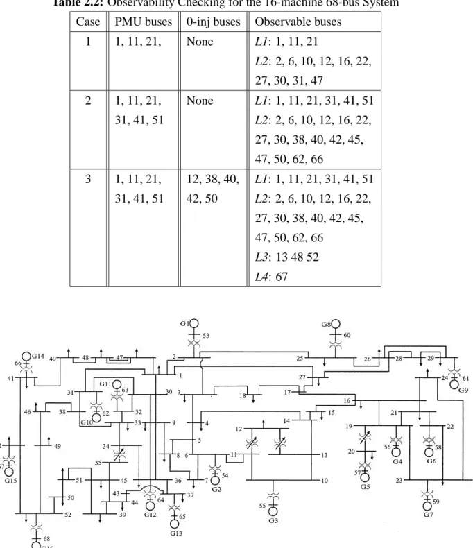
2.2 Observability Checking for the 16-machine 68-bus System . . . 36
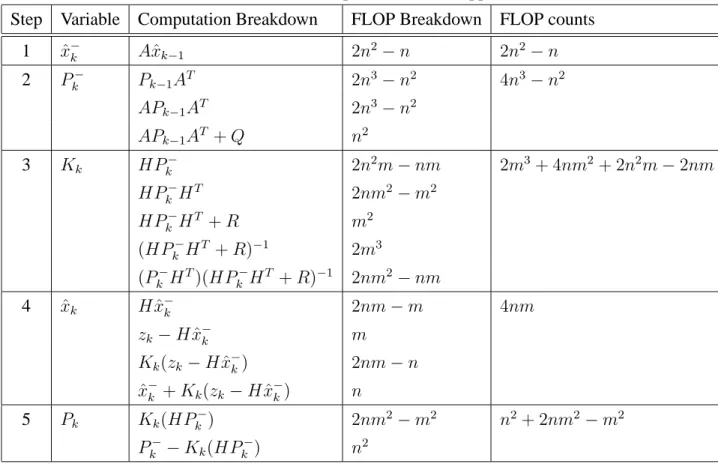
3.1 Kalman Filter Computational Cost Upper Bound . . . 66
LIST OF FIGURES
2.1 The two-portπ-model of a transmission line . . . 19
2.2 The 3-machine 9-bus system . . . 34
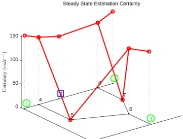
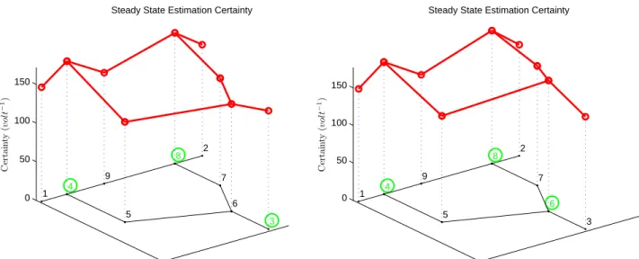
2.3 The certainty analysis plot of case 1 from Table 2.1, in the 3-machine 9-bus system . . . 35
2.4 The certainty analysis plot of case 2 from Table 2.1, in the 3-machine 9-bus system . . . 35
2.5 The certainty analysis plot of case 3 from Table 2.1, in the 3-machine 9-bus system . . . 35
2.6 The 16-machine 68-bus system . . . 36
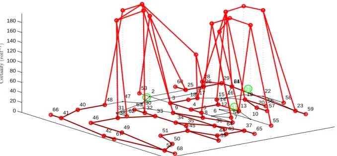
2.7 The certainty analysis plot of case 1 from Table 2.2, in the 16-machine 68-bus system . . . 37
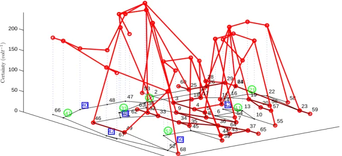
2.8 The certainty analysis plot of case 2 from Table 2.2, in the 16-machine 68-bus system . . . 37
2.9 The certainty analysis plot of case 3 from Table 2.2, in the 16-machine 68-bus system . . . 38
2.10 PMUs installed at buses 1, 6 and 8 . . . 39
2.11 PMUs installed at buses 2, 4 and 6 . . . 39
2.12 PMUs installed at buses 3, 4 and 8 . . . 39
2.13 PMUs installed at buses 4, 6 and 8 . . . 39
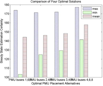
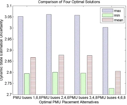
2.14 A comparison of steady-state certainties for the four “optimal" solutions, based upon three criteria: maximum (max), minimum (min) and average (mean). . . . 40
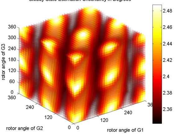
2.15 Steady-state estimation uncertainty versus rotor angles for the ideal case, i.e. when PMUs are installed on all buses. . . 47
2.17 Steady-state estimation uncertainty versus rotor angles for PMUs installed at
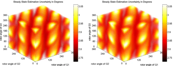
buses 2, 4 and 6. . . 48
2.18 Steady-state estimation uncertainty versus rotor angles for PMUs installed at buses 3, 4 and 8. . . 48
2.19 Steady-state estimation uncertainty versus rotor angles for PMUs installed at buses 4, 6 and 8. . . 48
2.20 The comparison of the four “optimal" solutions based upon three criteria: max, min and mean . . . 49
3.1 The operation of a discrete Kalman filter cycle . . . 60
3.2 Complexity-Speed-Change Cycle [1] . . . 64
3.3 The LoDiM algorithm flow chart. . . 74
3.4 Bus 2 Voltage magnitude estimation using conventional Kalman filter . . . 76
3.5 Bus 2 Voltage magnitude estimation using randomly chosen measurements . . . 77
3.6 Bus 2 Voltage magnitude estimation using LoDiM . . . 78
3.7 The performance comparison of state estimation with full measurement-space (in red), with randomly selected measurements (in green) and with LoDiM (in blue), fromt= 4tot = 6 . . . 79
3.8 Bus60Voltage magnitude estimation using conventional Kalman filter . . . 80
3.9 Bus60Voltage magnitude estimation using randomly chosen measurements . . 81
3.10 Bus 60Voltage magnitude estimation using our LoDiM method for measure-ment selection. . . 81
3.11 The performance comparison of different methods at generator bus 60in the 16-generator 68-bus system, with full measurement-space (in red), with ran-domly selected measurements (in green) and with LoDiM (in blue), fromt= 4 tot= 6 . . . 82
3.13 Performance comparison of LoDiM with different mσ values, at bus 2 in the
3-generator 9-bus system . . . 84
3.14 Performance comparison of LoDiM with differentmσ values, at bus 26 in the 16-generator 68-bus system . . . 84
3.15 LoDiM performance versus different amount of selected measurements in the 3-generator 9-bus system, with 10 megaFLOPS computing power available . . 85
3.16 LoDiM performance versus different amount of selected measurements in the 16-generator 68-bus system. with 1 gigaFLOPS computing power available . . 86
3.17 Estimation of rotor speed at generator 2 using ReMeDySE and regular EKF, with a 3-phase fault at bus 29 . . . 90
3.18 Performance comparison of ReMeDySE and regular EKF estimating rotor speed at generator 2, fromt= 2tot= 5 . . . 91
3.19 Performance comparison of ReMeDySE and regular EKF estimating rotor an-gle at generator 2, fromt= 2tot = 5 . . . 91
3.20 Performance comparison of ReMeDySE and regular EKF estimating rotor speed at generator 10, fromt= 2tot= 5 . . . 91
3.21 Performance comparison of ReMeDySE and regular EKF estimating rotor an-gle at generator 10, fromt= 2tot = 5. . . 91
4.1 High-level diagram of Kalman filter, courtesy of Greg F. Welch. System model error, and/or measurement error, can all lead to significant state estimation error when passing through a Kalman filter . . . 103
4.2 The circular boundary of a 1% TVE criterion . . . 109
4.3 Voltage estimation results of three filters in case 1 . . . 112
4.4 Voltage estimation accuracy of three filters in case 1 . . . 113
4.5 Voltage estimation results of three filters in case 1 . . . 115
4.6 Voltage estimation accuracy of three filters in case 2 . . . 116
4.9 Voltage estimation results of three filters in case 4 . . . 121
4.10 Voltage estimation accuracy of three filters in case 4 . . . 122
4.11 Voltage estimation results of three filters in case 5 . . . 124
4.12 Voltage estimation accuracy of three filters in case 5 . . . 125
4.13 Bus 1 voltage estimation results of three filters in case 6 . . . 128
4.14 Bus 4 voltage estimation results of three filters in case 6 . . . 129
4.15 Voltage estimation accuracy of three filters in case 6 . . . 130
4.16 Voltage estimation results of three approaches in case 1 . . . 140
4.17 Voltage estimation accuracy of three approaches in case 1 . . . 141
4.18 Rotor speed and angle estimation results of three approaches in case 1 . . . 142
4.19 Rotor speed estimation accuracy of three approaches in case 1 . . . 143
4.20 Rotor angle estimation results of three approaches in case 1 . . . 144
4.21 Voltage estimation results of three approaches in case 2 . . . 146
4.22 Voltage estimation accuracy of three approaches in case 2 . . . 147
4.23 Rotor speed and angle estimation results of three approaches in case 2 . . . 148
4.24 Rotor speed estimation accuracy of three approaches in case 2 . . . 149
4.25 Rotor angle estimation results of three approaches in case 2 . . . 150
4.26 Voltage estimation results of three approaches in case 3 . . . 152
4.27 Voltage estimation accuracy of three approaches in case 3 . . . 153
4.28 Rotor speed and angle estimation results of three approaches in case 3 . . . 154
4.29 Rotor speed estimation accuracy of three approaches in case 3 . . . 155
4.30 Rotor angle estimation results of three approaches in case 3 . . . 156
4.32 Voltage estimation accuracy of three approaches in case 4 . . . 159
4.33 Rotor speed and angle estimation results of three approaches in case 4 . . . 160
4.34 Rotor speed estimation accuracy of three approaches in case 4 . . . 161
4.35 Rotor angle estimation results of three approaches in case 4 . . . 162
4.36 Voltage estimation results of three approaches in case 5 . . . 164
4.37 Voltage estimation accuracy of three approaches in case 5 . . . 165
4.38 Rotor speed and angle estimation results of three approaches in case 5 . . . 166
4.39 Rotor speed estimation accuracy of three approaches in case 5 . . . 167
CHAPTER 1
INTRODUCTION
1.1
Motivations and Topics
From electrical power grids to economics, from microcontroller chips to spacecrafts,
sys-tems are everywhere and a part of everything. Either complex or simple, a system at a given
time point can be determined by a set of system variables. The smallest possible such set is
known as the internal state, or simply the state. Because the set of state variables can fully
specify the system at any give time, it is an essential element in system analysis and control.
While the true values of state variables may never be known exactly, they can be estimated
using the available measurements and established state models. From an engineering
per-spective, numerous professionals have devoted their efforts to developing advanced measuring
technologies and data processing technologies, so that measuring and computing devices are
constantly developing towards higher accuracy and greater efficiency.
Other than designing better measuring instruments, processing data on larger and faster
computational facilities, what else can we do to improve the estimation qualities? Here we
propose three topics from a computational and system-wide perspective:
• Grid Sensor Placement. When the measurement sensors are expensive/limited, it is
im-portant to install them at the most informative locations throughout the system network,
so that they can provide measurement data with optimal observability and reliability.
limited computational resources become obstacles in real-time state estimation, we hope
to reduce the computational complexity of the estimator. Strategic reduction of the
num-ber of measurements used per estimate allows us to do so without sacrificing the
estima-tion quality.
• Adaptive and Robust Estimation. In a hostile environment where the hypothetical models
do not match the actual systems, and/or the measurements contain significant errors, the
estimated states could deviate from the true states rapidly. The influenced estimation has
to be corrected as much as possible.
Our research on these topics, with applications in power systems, can serve as a bridge between
Computer Science and Power Engineering. Furthermore, they can be extended to other
large-scale complex systems as well. The background, previous work and our proposed ideas related
to these three topics will be explained in the following subsections.
1.1.1
Grid Sensor Placement
In our particular project we are dealing with advanced measurement sensors across the
power grid. Traditionally, power grid measurements are provided by remote terminal units
(RTUs) at the substations. RTU measurements include real/reactive power flows, power
injec-tions, and magnitudes of bus voltages and branch currents.
A novel phasor measurement technology was developed in the 1980s [2], [3]. The crucial
devices, called phasor measurement units(PMUs), are able to measure both magnitude and
phase angle of the electrical waves in a power grid. With the global positioning system (GPS),
PMU provide high-speed and high-accuracy sensor data with precise time synchronization.
While PMU measurements currently cover fewer than 1%of the nodes in the U.S. power
grid, the power industry actively invests in advancing the technology and installing more units.
However at the present stage, the installation must be selective because of resource constraints.
Previous PMU placement research has focused primarily on network topology, with the
goal of finding configurations that achieve full network observability with a minimum number
of PMUs [4, 5, 6, 7]. However we have noticed two issues about this problem: 1) The
observ-ability of the entire system is not an ˛aˇrall or nothing ˛a´s problem. PMUs are added to the grid
incrementally, and it will be useful to have some guidance on where to install them. 2) The
power system networks usually have complex topologies, so that when we obtain more than
one “optimal placement" solution with the same number of PMUs, one will have to make a
selection among these solutions.
To address these issues, recently we introduced an evaluation method that utilizes stochastic
models of the signals and measurements to characterize the observability and corresponding
uncertainty of power system states, for any given configuration of PMUs [8]. This evaluation
method includes a novel observability checking algorithm and estimation uncertainty analysis.
The observability checking classifies all the observable buses into one or more levels, according
to the ˛aˇrdirectness ˛a´s of their observations: Level 1 contains the most directly observable buses
(PMU buses), while the buses with more “indirect" (Section 2.8.1) observations are labeled
with higher levels. Then based on the previous work [9, 10], we compute a stochastic estimate
of the asymptotic or steady-state error covariance, P∞. P∞ is used as a quantitative metric for the performance evaluation. We generalize our approach for any PMU placement layout
without requirements for achieving full observability.
Because PMUs can provide real-time synchrophasor data to the Supervisory Control And
Data Acquisition (SCADA) system to capture the dynamic characteristics of the power system,
they have been found useful in estimating more transient states [11]. Thus we have extended
(generator rotor speed and rotor angles) state estimation applications. In [12], a new approach
is presented to design an optimal PMU placement according to estimation uncertainties of the
power system dynamic states. We restate the optimal PMU placement problem so that the
so-lution is not only a minimum set of PMUs that can cover the entire power system, but also
the one helps dynamic state estimation the most. So if an integer programming solver returns
multiple placement solutions, which all achieve full observability with the same minimum
number of PMUs, we apply steady-state uncertainty analysis to evaluate the solutions. The
op-timal PMU placement is hence selected according to the evaluation results. This approach can
provide planning engineers with a new tool to help in the selection between PMU placement
alternatives.
1.1.2
Filter Computation Adaptation
Dynamic state estimation (DSE) techniques, such as the Kalman filters [13], have been the
subject of extensive research and applications. Especially in modern power systems, DSE is a
fast developing research area. Compared to traditional steady state estimators, DSE techniques
are able to track dynamic state variables both efficiently and accurately.
However, in large-scale and wide-area inter-connected power systems, the combination of
high computational complexity and slow processing speed presents a significant challenge. To
help address this challenge, it is a good idea to employ faster response filters with reduced
measurement-space.
In our recent work we have set our sight on measurement-space reduction: we attempt to
select and process the measurement subsets which can improve state calculations the most. As
The LoDiM approach employs an estimator such as the Kalman filter, but with a twist:
while the filter is running in the foreground, it also performs a measurement selection procedure
in the background to optimally reduce the measurement dimension. The measurement selection
procedure utilizes the principal component analysis (PCA) of the error covariance, to determine
the subset of the state space to update most urgently (e.g. with larger estimation uncertainties
than others). We prefer to target at the principal uncertainties first, thus the measurements
are ranked according to their abilities to calibrate these uncertainties. Only a smaller subset
that can reduce the principal uncertainties most efficiently is then processed by the foreground
filter during each cycle. As a result, during each cycle it yields much smaller computational
load and hence lower latency. Furthermore, we have also extended our approach to Reduced
Measurement-space Dynamic State Estimation (ReMeDySE), for estimating the dynamic state
of power systems [17].
Although we present LoDiM in the context of the Kalman filter, the associated
measure-ment selection procedure is not filter-specific, i.e. it can be used with other state estimation
methods, as long as the state uncertainties are dynamically estimated along with the states.
Our approach is not application-specific either: it can be applied to other large-scale, real-time
on-line and computationally intensive state tracking systems with modern parallel computation
techniques.
1.1.3
Adaptive and Robust Estimation
Kalman filters achieve optimal performance only when the system noise characteristics
have known statistics that obey certain properties (zero-mean, Gaussian, and spectrally white).
However in practice, it is difficult to obtain the process and measurement noise models. When
the theoretical models do not match the actual models, and/or the measurements contain
estimated state deviate from true state, it is usually impossible to determine whether the
devia-tion is caused by a process model mismatch, a measurement model mismatch, or both.
To address this problem, we propose an efficient adaptive approach called the Adaptive
Kalman Filter (AKF) with Inflatable Noise Variances (InNoVa). Primary simulations have
demonstrated the robustness of this approach facing sudden changes of system dynamics and
erroneous measurements, with the ability to adjust noise modeling parameters on-the-fly. It is
capable of doing these because besides the regular normalized innovation test, we also employ
a normalized residual test to help separate the process and measurement factors.
Furthermore, we have considered incorporating AKF with InNoVa into the dynamic state
estimation algorithm from previous research [11], to also help with the estimation of power
system dynamic states. Thus we developed a two-stage Kalman filter approach to estimate the
static states of voltage magnitudes and phase angles, as well as the dynamic states of generator
rotor angles and generator speeds. In the first stage, we estimate the static states from raw
PMU measurements, using AKF with InNoVa, which is able to identify and reduce the impact
of incorrect system modeling and/or bad PMU measurements. Then in the next stage, the
estimated bus voltages are fed into a second extended Kalman filter to obtain the dynamic state
estimation. Case studies show the inherent advantages of our two-stage Kalman filter technique
over the extended Kalman filter alone.
1.2
Thesis Statement
to evaluate or optimize measurement unit placement in a network;
2. sensitivity-to-uncertainty ratio ranking can be used to select measurement subsets to optimally adapt to the available computational resources; and
3. innovation-residual tests can be used to identify apparent outlier measure-ments, and adapt the process/measurement models.
1.3
Contributions
• Our grid sensor placement approach is able to evaluate and compare any candidate sensor
placement configuration in complex networks, regardless of achieving full observability.
While off-line steady-state uncertainty analysis has aided in optimal sensor placement
for continuous-space systems such as the 3D tracking system, the combination of this
with a network topology analysis enables sensor placement evaluation and comparison
for discrete-space systems such as the power system.
• Our Lower Dimensional Measurement-space (LoDiM) state estimation algorithm,
adapt-ing to the computation budget available, can help many large-scale, real-time on-line and
computation-intensive state tracking systems because
1) it features a dynamic measurement selection procedure: a small measurement
subset is dynamically and strategically chosen for each cycle. The smaller
measurement-space incorporate less information per cycle, but has higher reporting rates;
2) the measurement selection procedure is not filter-specific, i.e. it can be used with
other state estimation methods such as particle and unscented filters.
• Our Adaptive Kalman Filter with Inflatable Noise Variances (AKF with InNoVa) enables
robust state estimation. Its ability of adjusting noise modeling parameters on-the-fly can
1) identify and adapt to incorrect system modeling;
2) identify and reduce the impact of erroneous measurements.
1.4
Thesis Organization
There are three main topics in this thesis. They are individually studied, yet closely related.
Among which, I investigate uncertainty-aware grid sensor placement stratagies in Chapter 2.
Next, Chapter 3 discusses how to use uncertainty-guided measurement selection approach to
reduce computational burden. Then I present our lately developed adaptive and robust state
estimation algorithms, based on uncertainty analyses, in Chapter 4. Finally, Chapter 5
summa-rizes our work, and proposes possible plans for the future research.
For each thesis topic, I will state the structure of its own chapter more specifically in the
CHAPTER 2
GRID SENSOR PLACEMENT
The synchronized phasor measurement unit (PMU), developed in the 1980s [2, 3], is
con-sidered one of the most important devices in the future of power systems. While PMU
measure-ments currently cover fewer than1% of the nodes in the U.S. power grid, the power industry
has gained the momentum to advance the technology and install more units. However, with
limited resources, the installation must be selective.
Previous PMU placement research has focused primarily on the network topology, with the
goal of finding configurations that achieve full network observability with a minimum number
of PMUs. Here we introduce a new approach that also includes stochastic models for the
signals and measurements, to characterize the observability and corresponding uncertainty of
any given configuration of PMUs, whether that configuration achieves full observability or not.
Utilization of this approach to designing optimal PMU placements, according to estimation
uncertainties of the power system static states/dynamic states, are also discussed in details.
This approach can provide planning engineers with a new tool to help choose between PMU
placement alternatives.
2.1
Introduction
State estimation plays a crucial role in determining the health of a power system. State
can be estimated using the available measurements and system model. Traditionally, remote
terminal units (RTU) at the substations provide power grid measurements. The most commonly
• Line power flow measurements: the real and reactive power flow along the transmission
lines or transformers.
• Bus power injection measurements: the real and reactive power injected at the buses.
• Voltage magnitude measurements: the voltage magnitudes of the buses.
Under certain circumstances such as state estimation of distribution systems, the line current
magnitude measurements may be considered, which provide the current flow magnitudes along
the transmission lines or transformers.
With the ability to impact future power system monitoring and operation methods, phasor
measurement technology is one of the key enabling technologies for the future “smart grid".
Phasor measurement units (PMUs) make two additional types of measurements available:
• Voltage phasor measurements: the phase angles and magnitudes of voltage phasors at
system buses.
• Current phasor measurements: the phase angles and magnitudes of current phasors along
transmission lines or transformers.
Recent development of phasor measurement technologies offers high-speed sensor data
(typi-cally 30 or 60 samples/second) with precise time synchronization. This is in comparison with
traditional RTU measurements in SCADA system, which have cycle times of 2 to 4 seconds
and are not well synchronized.
PMUs are becoming increasingly attractive in various power system applications such as
system monitoring, protection, control, and stability assessment. Widely scattered in the power
system network and synchronized from the common global positioning system (GPS) radio
such as dynamic state estimation and dynamic stability analysis [11]. Compared to estimating
relatively stationary state elements such as bus voltage magnitudes and phase angles, dynamic
state estimation seeks to estimate more transient states of a power system, i.e. generator rotor
angles and speeds. With properly placed and sufficient numbers of PMUs, we can estimate the
system status in real-time using time stamped synchrophasors.
There has been significant work in selecting the best locations to install PMUs [4, 5, 6, 7].
Many algorithms have been developed, primarily with the aim of utilizing a minimum number
of PMUs to ensure full network observability. However, two issues caught our attention:
• First, the observability of the entire system is not an “all or nothing” problem. Due to
various resource limitations, we do not have the luxury of installing a complete set of
PMUs throughout the power grid. Yet we are not starting from scratch either. In practice
people are installing PMUs to the grid incrementally, thus it would be useful to have
some guidance on where to install them.
• Second, in the previous research, the network topology was the primary focus. In practice
the networks usually have complex topologies where more than one solution for the same
minimum number of PMUs will appear. In such cases, the planning engineers need to
make a choice from these solutions.
We focus on bridging these gaps. Specifically our contributions include:
• We develop a stochastic model that captures state estimation uncertainties, to facilitate
PMUs installation assessment.
• We design an optimal PMU placement evaluation algorithm by incorporating uncertainty
estimates into topological considerations for the specific network.
• We present an approach to the comparison among alternative configurations via
2.2
Chapter Organization
The rest of this chapter is organized as follows. Section 2.3 introduces the background. In
Section 2.4 and Section 2.5, I review the basic concepts of state space models and steady state
estimation briefly. Section 2.6 discusses traditional power system state estimation method.
Section 2.7 describes the PMU devices and their impact on power system state estimation.
Then for static (Section 2.8) and dynamic (Section 2.9) state estimation respectively, we present
our approach to determine the effects of any given PMU configuration, and restate the optimal
PMU placement problem such that the solution is not only a minimum set of PMUs that can
cover the entire power system, but also the set that improves state estimation the most. Our
methods are simulated on multi-machine system models to demonstrate how it might help
engineers make decisions on different candidate plans.
2.3
Background and Related Work
The phasor measurement unit (PMU) was first developed and utilized in [2, 3].
Consid-ering partially observable systems (with an inadequate number of PMUs) the authors in [18]
presented an estimation algorithm based on singular value decomposition (SVD), which did
not require fully observable system prior to estimation.
Optimal PMU placement for full observability was studied in [4]. They developed an
algo-rithm for finding the minimum number of PMUs required for power system state estimation,
using simulated annealing optimization and graph theory in formulating and solving the
prob-lem.
PMUs using integer programming. In [5], a strategic PMU placement algorithm was developed
to improve the bad data processing capability of state estimation by taking advantage of the
PMU technology. Furthermore, [6] re-studied the PMU placement problem and presented a
generalized integer linear programming formulation.
Our work, however, is taking a different approach: we first characterize the observability
and corresponding uncertainty of the power system buses for any given configuration of PMUs,
whether that configuration achieves full observability or not. Then we also presented our work
on connecting the optimal PMU placement with power system static as well as dynamic state
estimation: we provide a method for evaluating any candidate PMU placement design, which
is especially useful when there are multiple placement candidates [8], [12].
2.4
State Space Models
The state space models are the most basic yet extensively used mathematical models in
all kinds of state estimation problems. Here I present a brief review to introduce the relevant
mathematical notations used throughout this dissertation. For more detailed description, the
readers can refer to [19].
An assumed linear system can be modeled as a set of linear stochastic process equation
and measurement equation:
xk =Axk−1+Buk−1+wk−1 (2.1)
zk =Hxk+vk (2.2)
wherex∈ Rn is the state vector,Ais an×nmatrix that relates the state at the previous time
stepk−1to the state at the current stepk, without either a driving function or process noise1,
u ∈ Rl is the optional control input vector. B is a n×lmatrix that relates the control input
vector to the state xk, z ∈ Rm is the measurement vector, H is am×n matrix that relates
the statexkto the measurementzk. w ∈ Rnandv ∈ Rmare process and measurement noise
vectors respectively.
The process noise w and measurement noise v are assumed to be mutually independent random variables, white, and with normal probability distributions:
p(w)∼N(0, Q) (2.3)
p(v)∼N(0, R) (2.4)
where the process noise covarianceQand measurement noise covarianceRmatrices are usu-ally assumed to be constant.
In reality, the process to be estimated and (or) the measurement relationship to the process
is usually non-linear. Especially when our objective is to estimate the dynamic states of the
power system. A non-linear system can be modeled using non-linear stochastic process and
measurement equations
xk =a(xk−1, uk−1) +wk−1 (2.5)
zk =h(xk) +vk. (2.6)
wherex∈ Rnis the state vector,ais a non-linear function that relates the state at the previous
time stepk−1to the state at the current stepk. uis the (optional) driving function, considered as parameters in function a. z ∈ Rm is the measurement vector. h is another non-linear
function that relates the statexkto the measurementzk. wandv again represent the zero-mean
process and measurement noise as defined before.
These non-linear functions can be linearized about the point of interestxin the state space. To do so one need to compute the state Jacobian and measurement Jacobian matrices
A= ∂a(x)
whereAandH are the partial derivatives ofaandh, with respect tox.
For any state estimatexˆk, we define the estimate error asek ≡xk−xˆk and estimate error
covariance asPk ≡E[ekeTk], whereE denotes statistical expectation. For the state estimatexˆk
at the time stepk, the estimate error covariance Pkcontains important information, reflecting
the uncertainty of the estimation.
2.5
Steady State Estimation
On-line methods such as the Kalman filter [13, 19] can be used to estimate time varying
state and error covariance, by minimizing the a posteriori estimate error covariance Pk in a
recursive predictor-corrector fashion. More details can be found in Section 3.4. In these
on-line scenarios the estimate error covariance Pk changes over time. However the steady-state
error covariance
P∞= lim
k→∞E[(xk−xˆk)(xk−xˆk)
T]
= lim
k→∞E[eke
T
k] (2.9)
can be computed off-line in closed form. Herexandxˆrepresent the true and estimated states respectively, andE denotes statistical expectation. In fact to compute the steady-state uncer-tainty one does not actually need to estimatexk andxˆk. Instead one can estimateP∞directly
from state-space models of the system using stochastic models for the various noise sources.
The rest of this section reviews the method for estimating P∞ based on previous work [9, 10], which employs the Discrete Algebraic Riccati Equation (DARE). The DARE represents
a closed-form solution to the steady-state covariance P∞ [20]. Assuming the process and measurement noise elements are uncorrelated, it can be written in this form:
The derivation of the DARE will be explained in Section 3.4.1.
The DARE solutionP∞ can be calculated using the MacFarlane-Potter-Fath “Eigenstruc-ture Method” [20]. Given the model parametersA,Q, H, andRfrom the last subsection, the
2n×2ndiscrete-time Hamiltonian matrix is written as
Ψ = ⎛ ⎜
⎝ A+QA
−THTR−1H QA−T
A−THTR−1H A−T ⎞ ⎟
⎠. (2.11)
Then after calculatingncharacteristic eigenvectors[e1, e2, ..., en]ofΨ, we form a matrix ⎛
⎜ ⎝ B
C
⎞ ⎟
⎠= [e1, e2, ..., en] (2.12)
Finally, we useB andC to compute the steady-state error covariance
P∞=BC−1. (2.13)
Note that if the JacobiansAandHare functions of the state, we will generally have to compute them at each point of interest in the state space. The noise covariance matricesRandQmight be constant, or might also vary as a function of the state.
For each point of interest in the state space, P∞ indicates the expected asymptotic state estimation uncertainty corresponding to the candidate design modeled by the specificA,Q,H, andR. Intuitively, given PMU placements leading to the same level of observability, the lower the overall uncertainty is, the more we prefer this design.
2.6
Traditional Power System State Estimation
SCADA system. Usually, people use weighted least squares (WLS) estimators to find the best
estimates of the states. In this subsection, we give a brief review of traditional power system
state estimation method and model, based on the classic textbook [21]. We refer this procedure
as a static state estimation because it obtains the voltage phasors at all buses at a single point
in time. In other words, WLS estimator only focuses on the measurement equations (2.2, 2.6)
in the state space model, without considering the process equations (2.1, 2.5).
2.6.1
Weighted Least Squares Estimator
The measurements used by the estimator are the real and reactive power flows and bus
injections, and the voltage magnitudes |V|, as provided by SCADA data. Traditionally the phase angles, θ, are not known. It is assumed that bad data have been eliminated from this measurement set by the usual methods. The measurements are usually formulated in vector
notation as
z =h(x) +v (2.14)
wherez is the measurement vector,xis the state vector,vis the vector of the measurement er-rors from noise, and the vector functionhis the nonlinearity between the power measurements and the state.
The WLS estimator aims at minimizing the objective functionJ, which is formulated as the sum of the squares of the weighted residuals:
J(x) = [z−h(x)]TR−1[z−h(x)] (2.15)
whereRis the measurement error covariance matrix. At thekth iteration of the WLS solution, the residual vectorris defined as
To minimize the objective functionJ, the first-order optimality conditions must be satisfied, that is
g(x) = ∂J(x)
∂x =−H
T(x)R−1[z−h(x)] = 0, (2.17)
where
H(x) = ∂h(x)
∂x (2.18)
is the Jacobian matrix obtained by taking partial derivatives ofhwith respect tox.
A non-linear optimization algorithm, such as the Newton-Raphson technique, is used to
iteratively converge to a solution. Assuming the Newton-Raphson method and the first-order
Taylor expansion are applied, along with an initial value of x, the step at each iteration k becomes:
xk+1 =xk+ [G(xk)]−1HT(xk)R−1[z−h(xk)], (2.19)
whereG(xk)is the gain matrix given by
G(xk) = ∂g(x
k)
∂x =H
T(xk)R−1H(xk).
(2.20)
The gain matrix is positive definite and symmetric provided that the system is fully observable,
and it is normally sparse.
The estimator is considered to have converged when the reduced-order measurement
mis-match vectorHT(xk)R−1[z−h(xk)]has reached some prescribed threshold.
sometimes line current magnitudes. These measurements can be expressed in terms of the state
variables either using the rectangular or the polar coordinates—the conventional choice is polar
coordinates. Here we briefly describe the measurement equations provided by [21].
If a system containsN buses, the state vector will have(2N −1)elements:N bus voltage magnitudes and(N −1)bus voltage phase angles, as one bus is chosen as the reference bus with its phase angle set equal to an arbitrary value such as 0. This bus is also known as the
slack bus or swing bus.
Typically we choose bus 1as the reference bus. The state vector will have the following
form:
x= [θ2θ3...θNV1V2...VN]T. (2.21)
Assuming the general two-portπ-model for the power system transmission lines (as shown in Fig. 2.1),
Figure 2.1: The two-portπ-model of a transmission line
• Real power injection at busi:
Pi =Vi N
j=1
Vj(Gijcosθij +Bijsinθij) (2.22)
• Reactive power injection at busi:
Qi =Vi N
j=1
Vj(Gijsinθij −Bijcosθij) (2.23)
• Real power flow from busito busj:
Pij =Vi2(gsi+gij)−ViVj(gijcosθij +bijsinθij) (2.24)
• Reactive power flow from busito busj:
Qij =−Vi2(bsi+bij)−ViVj(gijsinθij −bijcosθij) (2.25)
• Line current flow magnitude from busito busj:
Iij =
Pij2 +Q2ij Vi
(2.26)
Because in practice the shunt admittance gsi +jbsi is much smaller comparing to the
series admittancegij +jbij, the shunt admittance is usually ignored:
Iij = (gij2 +b2ij)(Vi2+Vj2−2ViVjcosθij) (2.27)
• Voltage magnitude at busi:
Vi =Vi (2.28)
where
θij =θi−θj is the phase angle difference between busesiandj,
gsi+jbsiis the shunt admittance connected at busi,
gij +jbij is the series admittance of the transmission line connecting busesiandj,
Gij +jBij is theijth element of the complex bus admittance matrix.
The measurement Jacobian matrixHthen has the following form:
H = ⎛ ⎜ ⎜ ⎜ ⎜ ⎜ ⎜ ⎜ ⎜ ⎜ ⎜ ⎜ ⎜ ⎜ ⎜ ⎝ ∂Pinj ∂θ ∂Pinj ∂V
∂Pf low
∂θ
∂Pf low
∂V
∂Qinj
∂θ
∂Qinj
∂V
∂Qf low
∂θ
∂Qf low
∂V
∂Imag
∂θ
∂Imag
∂V
0 ∂Vmag
∂V ⎞ ⎟ ⎟ ⎟ ⎟ ⎟ ⎟ ⎟ ⎟ ⎟ ⎟ ⎟ ⎟ ⎟ ⎟ ⎠ . (2.29) where
Pinj andQinj are the real and reactive power injection measurements,
Pf lowandQf loware the real and reactive power flow measurements,
Imag andVmag are the line current flow magnitude and voltage magnitude measurements.
• Partial derivatives of real power injection at busi: ∂Pi ∂θi = N j=1
ViVj(−Gijsinθij +Bijcosθij)−Vi2Bii (2.30)
∂Pi
∂θj
=ViVj(Gijsinθij −Bijcosθij) (2.31)
∂Pi ∂Vi = N j=1
Vj(Gijcosθij +Bijsinθij) +ViGii (2.32)
∂Pi
∂Vj
=Vi(Gijcosθij +Bijsinθij) (2.33)
• Partial derivatives of reactive power injection at busi:
∂Qi ∂θi = N j=1
ViVj(Gijcosθij +Bijsinθij)−Vi2Gii (2.34)
∂Qi
∂θj
=ViVj(−Gijcosθij −Bijsinθij) (2.35)
∂Qi ∂Vi = N j=1
Vj(Gijsinθij −Bijcosθij)−ViBii (2.36)
∂Qi
∂Vj
=Vi(Gijsinθij −Bijcosθij) (2.37)
• Partial derivatives of real power flow from busito busj:
∂Pij
∂θi
=ViVj(gijsinθij −bijcosθij) (2.38)
∂Pij
∂θj
=−ViVj(gijsinθij −bijcosθij) (2.39)
∂Pij
∂Vi
=−Vj(gijcosθij+bijsinθij) + 2(gij+gsi)Vi (2.40)
∂Pij
∂Vj
• Partial derivatives of reactive power flow from busito busj:
∂Qij
∂θi
=−ViVj(gijcosθij +bijsinθij) (2.42)
∂Qij
∂θj
=ViVj(gijcosθij +bijsinθij) (2.43)
∂Qij
∂Vi
=−Vj(gijsinθij−bijcosθij)−2(bij +bsi)Vi (2.44)
∂Qij
∂Vj
=−Vi(gijsinθij −bijcosθij) (2.45)
• Partial derivatives of line current flow magnitude from busito busj, shunt admittance ignored:
∂Iij
∂θi
= gij2 +b2ij
Iij
ViVjsinθij (2.46)
∂Iij
∂θj
=−gij2 +b2ij
Iij
ViVjsinθij (2.47)
∂Iij
∂Vi
= gij2 +b2ij
Iij
(Vi−Vjcosθij) (2.48)
∂Iij
∂Vj
= gij2 +b2ij
Iij
(Vj−Vicosθij) (2.49)
• Partial derivatives of voltage magnitude at busi:
∂Vi
∂Vi
= 1 (2.50)
∂Vi
∂Vj
= 0 (2.51)
∂Vi
∂θi
= 0 (2.52)
∂Vi
∂θj
= 0 (2.53)
2.7
The Phasor Measurement Units (PMUs)
Synchronized by GPS satellite clock, PMUs have achieved a level of precision that typically
measurements. Nowadays, PMUs are becoming more and more attractive in various power
system applications such as system monitoring, protection, control, and stability assessment.
The benefit of PMUs is especially evident when it comes to power system state estimation.
Conventional power system state estimation uses real and reactive power as measurements
to estimate the bus phasor voltages. As a result, the relationship between measurements and
states is non-linear. The solution is always obtained by linearizing the model and solving it in
an iterative fashion.
PMUs alleviate this problem by providing the phasors of voltages and currents measured
at a given substation. Hence, by measuring the bus phasor voltages and line phasor currents,
the relationship between measurements and states becomes linear. When the measurement
equation is linear, the estimation algorithm is direct and significantly faster than the non-linear
ones.
2.7.1
Observability Checking
For modeling power systems, we consider two types of measurements: PMU measurements
and zero injection measurements.
A PMU installed at a specific bus is capable of measuring not only the bus voltage phasor,
but also the current phasors along all the lines incident to the bus. Hence in addition to the
phasor voltage at this bus, we are able to compute the phasor voltages of all of its neighboring
buses.
If a bus has neither generators nor loads, it is a zero injection bus [21]. The inclusion of
measurement [7], which is useful in system state estimation. According to Kirchhoff’s current
law, we know that at any bus in the power grid, the sum of currents flowing into that bus is
equal to the sum of currents flowing out of that bus. Thus, for an injection-measured bus and
itsnneighbors ((n+ 1)buses total), if the phasor voltages at anynout of the(n+ 1)buses are known (observable), then the remainder can also be computed and hence become observable.
Consistent with previous studies, we only consider isolated zero injection buses in our test
systems. Meaning that, once a zero injection bus location is used in our algorithm, other zero
injection buses adjacent to it (if there is any) will not be taken into account. This is because
although zero injection buses can help reduce the PMUs needed for a system, the reduction of
PMUs will compromise the system reliability. More detailed explanation can be found in [22].
Based on these assumptions, we have developed the observability checking algorithm shown
in Algorithm 1.
2.8
My Method: PMU Placement for Power System Static State
Estima-tion
2.8.1
PMU Placement Evaluation
Previous studies consider a PMU placement optimal in the sense that it maximizes
observ-ability while minimizing cost. The authors in [6, 7] presented a numerical formulation of this
problem, and developed an optimal placement algorithm for PMUs using integer linear
pro-gramming. This formulation allows easy analysis of the network observability and concerns
about the full coverage of the system. However, the integer linear programming approach may
be insufficient for determining the optimal locations of PMUs. The reason is that very often
Algorithm 1: Observability checking for a given set of PMU locations and zero injection buses.
Input: PMU buses locationP_busand zero injection buses locationZ_bus Output: Observable buses locationO_bus
O_bus=∅;
O_bus=P_bus(the buses that can be measured directly by PMUs); fori←1to|P_bus|do
O_bus=O_bus∪neighbors(P_busi)
(the| · |operator denotes the cardinality of the set);
(adding the buses that can be estimated through at least one adjacent PMU bus); f lag = 1;
while flag do f lag = 0;
forj ← 1to|Z_bus|do if
(|Z_busj∪neighbors(Z_busj))∩O_bus|=|Z_busj∪neighbors(Z_busj)|−1
then
O_bus=O_bus∪Z_busj∪neighbors(Z_busj);
f lag = 1;
(adding the buses that can be estimated using the zero injection information. According to the Kirchhoff’s law: for a zero injection bus and its
neighborhood, if all but one is known, then the unknown one can be estimated );
cases, one would need a means for comparing the different solutions, as some will actually
offer lower estimate uncertainty and latency.
Built on the previous work by Allen et al. [9, 10], our approach is to use a stochastic
estimate of the asymptotic or steady-state error covariance, as a quantitative metric for the
performance evaluation. Our approach is generalized for any PMU placement layout, without
requirements for achieving full observability.
To estimate the steady-state error covariance, we first consider the relevant state space
The Process Model
For modeling the state and covariance changes over time, there are several ways to
iden-tify the parameters A andQ, both a priori and on-line [10, 20]. Following the methodology described in [23], a quasi-static model of an assumingly stable power system is used in our
ap-proach. The oscillations in the state variables of this model are assumed small, thus the states
of the power system at time step(k+ 1)are the same as those at time stepk, except for some zero mean, white Gaussian noise. Hence our process model reduces to
xk =xk−1+wk−1. (2.54)
The Measurement Model
Traditionally, real and reactive power measurements are used in the power system state
estimation, resulting in non-linear measurement models and iterative algorithm to solve for the
state of the system. Now with the help of PMUs, the measurement model becomes linear: we
simply let the phasor bus voltages be the state, while phasor bus voltages and phasor currents
be the measurements. In this way we are able to use non-iterative estimation algorithms, which
speeds up the computation signficantly.
The measurement model has the general form
z=Hx+v, (2.55)
wherex ∈ Rn is the complex state vector,z ∈ Rm is the complex measurement vector, and
H is am×n complex matrix that relates the state to the measurementzk. The measurement
noise elements invare assumed to be mutually independent random variables, white, and with normal probability distributions
For computational convenience, we convert the complex valued measurement model into a real
valued measurement model as in [18]:
⎛ ⎜
⎝ Re(z)
Im(z)
⎞ ⎟ ⎠=
⎛ ⎜
⎝ Re(H) −Im(H)
Im(H) Re(H)
⎞ ⎟ ⎠
⎛ ⎜
⎝ Re(x)
Im(x)
⎞ ⎟ ⎠ + ⎛ ⎜
⎝ Re(v)
Im(v)
⎞ ⎟
⎠ (2.57)
whereRe(·)andIm(·)stand for the real and imaginary parts of the corresponding vector/matrix respectively.
After the procedure of observability checking, all the observable buses are divided into one
or more levels, according to the “directness” of their observations: with Level 1 containing
the most directly observable buses, and the buses with more “indirect” observations labeled
with higher levels. Note that if the power grid only uses PMU measurements, the observable
buses belong to either Level 1 or Level 2; however, if both PMU measurements and injection
measurements (which could be zero injection pseudo-measurements) are taken into account,
there may be more than two levels of observable buses.
Level 1 buses
If the busiis in Level 1 (meaning that there is a PMU placed on this bus), the measurement equation is
zi =xi+vi, (2.58)
whereziis the measured complex voltage at busi,xiis the “true” complex voltage at busiand
vi is the complex measurement noise of this PMU. Thus for all the buses in Level 1, we can
where zV is the complex voltage measurement subvector,I is the identity matrix, xL1 is the
complex state subvector (“true” complex voltages at all Level 1 buses) and vV is the voltage
measurement noise subvector.
Level 2 buses
If the busiis in Level 2 (meaning that there is at least one PMU placed on an adjacent bus), then for each PMU placed at some adjacent busj, the measurement equation will be
zji =
Yji −Yji ⎛
⎜ ⎝ xj
xi ⎞ ⎟
⎠+vj, (2.60)
where zji is the measured complex current at busj (towards busi), Yji is the admittance of
line(j, i), xj andxi are the “true” complex voltages at busj andirespectively, and vj is the
complex measurement noise of this PMU. So for all the buses in Level 1 and Level 2, we have
the measurement equation
zC =
YCL1 YCL2
⎛ ⎜ ⎝ xL1
xL2
⎞ ⎟
⎠+vC, (2.61)
where zC is the complex current measurement subvector, YCL1 and YCL2 are the line
admit-tance matrices that relates Level 1 and Level 2 bus voltages to zC respectively,xL1 andxL2
are the complex state subvector (“true” complex voltages at all Level 1 and Level 2 buses),
andvC is the current measurement noise subvector. In this equation, the measurement matrix
YCL1 YCL2
has each row sum up to zero. If the number of PMUs installed is sufficient,
or the power grid is well-connected, it is quite possible that a Level 2 bus has more than one
PMU-installed neighbor buses. In such cases, the measurement equation has fused the
Level 3 or above buses
If the busiis in Level 3 or above (meaning that we can compute the bus voltage, but there is no PMU placed on itself or any adjacent bus), then we must use the information about net
injection current measurements, and Kirchhoff’s Current Law, to calculate the complex bus
voltage. Generally there are two possibilities:
• an injection measurement is taken at busi; or
• an injection measurement is taken at busj, which is adjacent to busi.
Overall, assuming there are totallyl levels of observable buses, the measurement equation can be written as
zI =
YIL1 YIL2 YIL3· · · YILl
⎛ ⎜ ⎜ ⎜ ⎜ ⎜ ⎜ ⎜ ⎝
xL1
xL2
.. .
xLl
⎞ ⎟ ⎟ ⎟ ⎟ ⎟ ⎟ ⎟ ⎠
+vI, (2.62)
wherezI is the complex injection current measurement subvector (zero pseudo-measurements),
YIL1 throughYILl are the node admittance matrices of all observable buses that are related to
zI, xL1 throughxLl represent the complex state subvector for all observable buses, andvI is
Combining the above three cases, the complete measurement model can be expressed as ⎛ ⎜ ⎜ ⎜ ⎜ ⎝ zV zC zI ⎞ ⎟ ⎟ ⎟ ⎟ ⎠= ⎛ ⎜ ⎜ ⎜ ⎜ ⎝
I 0 0· · · 0
YCL1 YCL2 0· · · 0
YIL1 YIL2 YIL3· · · YILl
⎞ ⎟ ⎟ ⎟ ⎟ ⎠ ⎛ ⎜ ⎜ ⎜ ⎜ ⎜ ⎜ ⎜ ⎝
xL1
xL2
.. .
xLl
⎞ ⎟ ⎟ ⎟ ⎟ ⎟ ⎟ ⎟ ⎠ + ⎛ ⎜ ⎜ ⎜ ⎜ ⎝ vV vC vI ⎞ ⎟ ⎟ ⎟ ⎟
⎠. (2.63)
The measurement model can be converted into real valued model, using the technique
men-tioned before.
2.8.2
Optimal PMU Placement
Conventionally, the PMU placement is considered optimal in the sense that it makes all
buses in the system observable with a minimum number of PMUs. This is especially true for
large-scale complex systems. The authors in [6, 7] presented a numerical formulation of this
optimization problem:
min
n(buses)
i
wi·Xi (2.64)
s.t. f(X) =C·X ≥ˆ1
wheren(buses)is the number of buses in the system,wiis the cost of the PMU installed at bus
i,Xis a binary decision variable vector with entriesXidefined as
Xi = ⎧ ⎪ ⎨ ⎪ ⎩
1 if a PMU is installed at busi
0 otherwise
ˆ1is a vector whose entries are all ones, f(X)is a vector function andC is the binary
connec-tivity matrix with entries
C[k,m]= ⎧ ⎪ ⎪ ⎪ ⎪ ⎨ ⎪ ⎪ ⎪ ⎪ ⎩
1 ifk =m
1 if buseskandmare connected
0 otherwise
. (2.66)
This formulation allows easy analysis of the network observability and concerns about the
full coverage of the system. We first solve this optimization problem using integer linear
pro-gramming techniques. However, the integer linear propro-gramming approach is insufficient for
determining the optimal locations of PMUs. The reason is that very often there will be
multi-ple “optimal" solutions with the same minimum number of PMUs. In such cases, one would
need a means for comparing the different solutions, as some will actually offer lower estimate
uncertainty and latency.
Thus the next step is to evaluate the solution(s) using steady-state uncertainty analysis as
described in section 2.5. Naturally, we prefer the solution with lower uncertainties. If there
is no “absolute winner", (i.e. at each bus, the uncertainty value computed for this solution is
lower than any other solution), the user need to define a criterion to judge each solution, and
we will discuss more in the next section. Briefly, our approach for optimal PMU placement
using uncertainty evaluation can be described by Algorithm 2.
2.8.3
Simulation Results
In this section, we first apply our observability checking and estimation uncertainty analysis
to two simulated multi-machine systems. We then apply our approach to evaluate four different