FUNGIBLE PARAMETER CONTOURS AND CONFIDENCE REGIONS IN STRUCTURAL EQUATION MODELS
Jolynn Pek
A dissertation submitted to the faculty of the University of North Carolina in partial fulfillment of the requirements for the degree of Doctor of Philosophy in the Depart-ment of Psychology of
Chapel Hill 2012
Approved by:
Daniel J. Bauer Kenneth A. Bollen Robert C. MacCallum Keith Payne
c
2012
Jolynn Pek
ABSTRACT
JOLYNN PEK: Fungible Parameter Contours and Confidence Regions in Structural Equation Models
(Under the direction of Robert C. MacCallum)
There are at least two kinds of uncertainty associated with parameter estimates when statistical models are fit to sample data. The first kind of uncertainty is typically con-veyed by confidence regions which provide a plausible range of values for population parameters of interest. The second kind of uncertainty involves a sensitivity analysis (Cook, 1986) with respect to model fit. Here, contours representing alternative so-lutions for parameter estimates that are almost as good as the optimal estimates in terms of model fit are obtained. Contours of these slightly suboptimal parameter val-ues have been termed fungible weights or contours (Waller, 2008; Waller & Jones, 2009; MacCallum, Browne & Lee, 2009). Although distinct from each other, confidence re-gions and fungible contours communicate parameter uncertainty and are both com-puted from the likelihood function. Given these commonalities, we set out to clarify the relationship between confidence regions and fungible parameter contours by accom-plishing three objectives.
ACKNOWLEDGEMENTS
TABLE OF CONTENTS
LIST OF TABLES . . . xi
LIST OF FIGURES . . . xii
Chapter 1 INTRODUCTION . . . 1
1.1 Structural Equation Models and Maximum Likelihood Estimation . . . 5
1.2 Constructing Confidence Regions and Fungible Contours . . . 6
1.2.1 Likelihood-Based Confidence Regions . . . 6
1.2.2 Fungible Parameter Contours . . . 9
1.3 Computing Confidence Regions and Fungible Contours . . . 11
1.3.1 Existing Algorithms for Likelihood-Based Con-fidence Regions . . . 11
1.3.2 Estimating Fungible Contours . . . 12
1.3.3 Obtaining Confidence Regions via the Brent (1973) Algorithm . . . 13
1.5 Accounting for Nuisance Parameters . . . 18
1.5.1 Profile Likelihood Method . . . 19
1.5.1.1 Profile Likelihood-Based Confidence Bounds . . . 20
1.5.1.2 Profile Likelihood-Based Fungible Parameter Contours . . . 21
1.5.2 Marginal and Conditional Likelihood Methods . . . 21
1.6 Likelihood-Based Estimation in Practice . . . 22
1.7 An Empirical Demonstration . . . 24
1.7.1 Direct Effect (k = 1 ) . . . 26
1.7.2 Indirect Effect (k = 2 ) . . . 27
1.7.3 Summary and Extensions . . . 31
2 METHODS . . . 33
2.1 Modelling Factors that May Impact Parameter Uncertainty . . . 33
2.1.1 Population Generating Models . . . 35
2.1.1.1 Magnitude of Correlations . . . 36
2.1.1.2 Model Fit . . . 39
2.1.1.3 Sample Size . . . 41
2.1.2 Study Conditions . . . 41
2.2 Perturbation Schemes . . . 44
2.3 Profile and Empirical Likelihood-Based Computation . . . 45
2.4.1 Sample Size . . . 46
2.4.2 Model Fit . . . 47
2.4.3 Magnitude of Correlations . . . 47
2.4.4 Population Covariances . . . 49
2.4.5 Profile and Empirical Likelihood-Based Computation . . . 49
3 RESULTS . . . 51
3.1 Preliminary Analysis Evaluating Generated Data . . . 51
3.1.1 Correlations among Measured Variables . . . 51
3.1.2 Model Fit in Terms of Covariance Residuals . . . 53
3.1.3 Maximum Likelihood Estimates of Model Fit . . . 54
3.2 Relationship among Different Kinds of Perturbations . . . 55
3.3 Factors that Impact Parameter Uncertainty . . . 59
3.3.1 Sample Size . . . 65
3.3.2 Model Fit . . . 68
3.3.3 Magnitude of Correlations . . . 71
3.4 Population Covariances . . . 76
3.5 Profile and Empirical Likelihood-Based Computations . . . 79
4 DISCUSSION . . . 83
4.1 General Perturbation Framework . . . 83
4.2 Factors that Impact Parameter Uncertainty . . . 86
4.2.2 Likelihood Surface . . . 89
4.3 Computational Procedure . . . 90
4.3.1 Empirical Likelihood . . . 91
4.3.2 Profile Likelihood . . . 92
4.4 Study Contributions . . . 92
4.5 Future Directions . . . 93
4.6 Conclusion . . . 95
APPENDICES. . . 96
LIST OF TABLES
Table
1 Proposed Simulation Study Conditions . . . 43
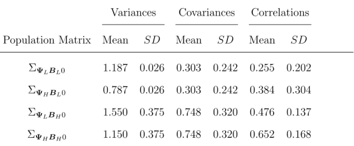
2 Descriptive Statistics of Elements within Population Matrices . . . 52
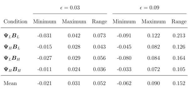
3 Range of Standardized Population Residuals . . . 53
4 Model Fit Information for Study Conditions . . . 55
5 Perturbation Values in Different Scales . . . 56
6 Major and Minor Axis across Model Fit . . . 66
7 Major and Minor Axis for Two Sets of Fungible Pa-rameter Contours . . . 70
8 Major and Minor Axis by Magnitude of Correlations among MVs . . . 74
9 Descriptive Statistics of Major and Minor Axes for the Two Sets of Fungible Parameter Contours . . . 78
LIST OF FIGURES
Figure
1 Path Diagram for Schmitt et al. (2002) Mediation Model . . . 25 2 Profile Likelihood-Based Confidence Bounds and
Fun-gible Contours for the Indirect Effect of Perceived
Dis-crimination on Well-being. . . 28
3 Profile Likelihood-Based Confidence Bounds and
Fun-gible Contours of β2,1 and β3,2 for ΨLBL. . . 61
4 Profile Likelihood-Based Confidence Bounds and
Fun-gible Contours of β2,1 and β3,2 for ΨHBL. . . 62
5 Profile Likelihood-Based Confidence Bounds and
Fun-gible Contours of β2,1 and β3,2 for ΨLBH. . . 63
6 Profile Likelihood-Based Confidence Bounds and
Fun-gible Contours of β2,1 and β3,2 for ΨHBH. . . 64
7 Profile Likelihood-Based Confidence Bounds and Fun-gible Contours of β2,1 and β3,2 by Magnitude of
Cor-relations among Measured Variables. . . 65 8 Profile Likelihood-Based Confidence Bounds and
Fun-gible Contours of β2,1 and β3,2 by Model Fit and
Sam-ple Size. . . 72 9 Profile Likelihood-Based Fungible Contours of β2,1
and β3,2 for ΨLBL and ΨHBH by Model Fit and
Sample Size. . . 77 10 Estimated and Profile Likelihood-Based Confidence
Chapter 1
INTRODUCTION
A major goal of statistical modelling is to obtain parameter estimates that summarize regularity inherent in the data at hand. Such parameter estimates allow researchers to describe, understand, explain and predict complicated phenomena. Yet, parameter estimates carry different kinds of uncertainty which should be taken into account when these estimates are to be rigorously interpreted or applied.
regions promote cross-validation. Clearly, strong scientific conclusions require small sampling variability (Green, 1977).
A second kind of uncertainty associated with parameter estimates may be in-vestigated via a sensitivity analysis (Cook, 1986). Sensitivity analysis involves intro-ducing practically insignificant changes to modelling conditions and assessing their ef-fects on study results. One form of sensitivity analysis examines the relationship be-tween parameter estimates and model fit. Specifically, parameter uncertainty is inves-tigated with respect to small perturbations introduced to model fit. Given a slightly suboptimal model fit, alternative solutions for parameter estimates may be obtained. Such alternative parameter values have been called exchangeable or “fungible” in that each set is associated with the same suboptimal model fit (Waller, 2008; Waller & Jones 2009). When a single parameter is involved, two fungible values are obtained. When more than one parameter is concerned, an infinite number of alternative solu-tions may be obtained. Uncertainty is couched as the degree of variation across dif-ferent combinations of parameter values that give practically the same, albeit slightly worse, model fit as the unique optimal solution. Stated differently, fungible parame-ter contours convey information on parameparame-ter variation, given a slightly suboptimal model fit. If the size of parameter values change radically under a minute perturbation to model fit, such parameter values provide a weak basis for scientific conclusions.
frame-work of structural equation models (SEMs) of which linear regression is a special case (MacCallum, Browne, & Lee, 2009). Indeed, the developments by these researchers are generalizable to virtually any statistical model.
Both tight confidence regions and tight fungible parameter contours promote strong scientific conclusions. Under maximum likelihood (ML) estimation, confidence regions or bounds and fungible contours are both based on the likelihood function which carries information regarding uncertainty associated with parameter estimates. While these two kinds of parameter uncertainty are distinct, these commonalities raise a need for clarification regarding the relationship between confidence regions and fungi-ble contours. As such, there are three objectives of the study. First, we will examine the analytical relationship between confidence regions and fungible contours in the context of SEMs. Second, we propose to develop computational methods to obtain likelihood-based confidence regions and fungible parameter contours for more than one parameter. Third, an investigation is conducted on how these two kinds of uncertainty are influenced by aspects of the data and model. The following is an overview of the study.
parameter values. Under this general theoretical framework, we will establish condi-tions under which confidence regions and fungible parameter contours are numerically identical, and summarize the similarities and differences between confidence regions and fungible contours.
Practical issues concerning the estimation of confidence regions and fungible contours are also discussed. In particular, computational difficulties arise when the number of parameters involved in computations is not small. Typically, analysts are interested in a small number of focal parameters and treat the remaining non-focal pa-rameters as nuisance papa-rameters. We will review several approaches to dealing with nuisance parameters and focus on the estimated likelihood and profile likelihood meth-ods to address the presence of nuisance parameters. We will then describe a root find-ing algorithm (Brent, 1973) to obtainfind-ing confidence regions and fungible parameter contours from both the estimated likelihood and the profile likelihood. An empirical example based on published data (Schmitt, Branscombe, Kobrynowicz, & Owen, 2002) is used to demonstrate this computational method as well as illustrate the relationship between confidence regions and fungible parameter contours.
1.1 Structural Equation Models and Maximum Likelihood Estimation
To set the framework and establish notation, we first review the structural equation model (SEM) and maximum likelihood (ML) estimation of these model pa-rameters. Structural equation models are multi-parameter models involving a hypoth-esized network of directional and non-directional relationships among sets of measured and latent variables (MVs and LVs). The p×p population covariance matrix of the MVs is typically denoted by Σ and the model implied k ×1 vector of parameters is denoted by θ. We will focus on covariance structure models, although our develop-ments may be extended to model mean structures. The SEM is simply expressed as Σ = Σ(θ) , implying that the population covariance matrix for the MVs is a func-tion of the model parameters. Parameter estimates ˆθ are computationally obtained by minimizing the discrepancy between the model implied population matrix Σ(θ) and the sample covariance matrix S.
There are many discrepancy functions for obtaining SEM parameter estimates such as the generalized least squares (GLS) and the asymptotically distribution free (ADF; Browne, 1984) approaches. However, the method of ML is the most commonly used technique. The multivariate normal likelihood function L(θ) to be maximized is defined by the specified model parameters θ and the data at hand. Note that L(θ) is a nonlinear expression of Σ(θ) . In practice, a monotonic transformation of the mul-tivariate normal likelihood function L(θ) , known as the ML discrepancy function F, is optimized to obtain ˆθ. Maximizing L(θ) is equivalent to minimizing F. The ML discrepancy function is
F(Σ,S) = ln|S|+ tr(SΣ−1)−ln|Σ| −p (1)
The estimated sample discrepancy function is given by ˆF = F(Σ(ˆθ),S) . Mul-tiplying ˆF by (N −1) , where N is the sample size, obtains the goodness-of-fit test statistic under the Wishart distribution (Browne & Arminger, 1995). This test statistic
T = (N −1) ˆF (2)
asymptotically follows a χ2 distribution with p(p+ 1)/2−k degrees of freedom under the null hypothesis that the model impled covariance matrix Σ(θ) is no different from the population covariance matrix Σ. Recall that k is the total number of parameters estimated under the specified model. This goodness-of-fit test statistic is also known as a likelihood ratio test (LRT) as this statistic compares the likelihoods of the specified model against the saturated model or the model which perfectly reconstructs the data (Bollen, 1989).
1.2 Constructing Confidence Regions and Fungible Contours
1.2.1 Likelihood-Based Confidence Regions
A useful supplement to ML point estimates is a confidence region, which con-veys the sampling variability that underlies parameter estimates. Besides likelihood-based confidence regions, there exist other approaches to constructing confidence re-gions such as the standard Wald approach. Suppose that a confidence interval for a single parameter is desired. Wald-type confidence intervals are constructed using the formula: estimate ± percentile × standard error of estimate. Here, the percentile is determined by some chosen confidence or error rate α and a reference distribution such as the normal distribution. Wald-type confidence intervals, however, perform poorly when the distribution of the parameter estimate is markedly skewed or if the estimated standard error is inaccurate (Stryhn & Christensen, 2003).
statistic or Lagrange Multiplier test. Score-type confidence regions are constructed us-ing the same formula as Wald-type confidence regions. While the percentile for both the Wald-type and Score-type confidence regions are the same, the estimate and stan-dard error of the estimate for the Score approach are distinct from the Wald method. In particular, Wald-type standard errors are obtained from the second derivatives of the likelihood function (or Hessian matrix) while Score-type standard errors are com-puted from the first derivatives of the likelihood function (or Gradient matrix). Score-type confidence regions suffer the same shortcomings as Wald-Score-type confidence regions as these two approaches are based on quadratic approximations to the log-likelihood (Meeker & Escobar, 1995). Perfect conformity of the log-likelihood to the quadratic form is rare in SEMs (Neale & Miller, 1997). Therefore, we will investigate likelihood-based confidence regions here.
Likelihood-based confidence intervals are constructed by inverting a certain type of LRT as described below. Suppose a likelihood-based confidence region for the k×1 vector of parameter estimates is desired. The null hypothesis tested by the LRT is H0 : θ = θ0 where θ0 is a k ×1 vector of population parameter values determined by the null hypothesis. Formally, this LRT is defined as
G2 = 2[l(ˆθ)−l(θ0)] (3)
where l(ˆθ) is the log-likelihood associated with the k ×1 vector of ML estimates and l(θ0) is the log-likelihood associated with the k ×1 vector of parameter values deter-mined by the null hypothesis. The test statistic G2 is asymptotically distributed as χ2 with k degrees of freedom under the null hypothesis.
There-fore, the likelihood-based confidence region is determined by solving for values of θ0 which satisfy the inequality
G2 ≤χ21−α,k. (4)
In this vein, the bounds or limits to likelihood-based confidence regions are obtained by solving for values of θ0 such that Equation 4 is an equality or G2 = χ21−α,k. Note
that when the null hypothesis is false, the appropriate statistic approximately follows a noncentral χ2 distribution with k degrees of freedom and a noncentrality parame-ter λ that depends on the alternative hypothesis that is taken to be true. Although confidence regions may be constructed using the noncentral χ2 distribution, when the null hypothesis is not true, implementation of this approach would require the user to specify some value of λ reflecting the degree of model misfit in the population. As this task could be problematic in practice, we will focus on inverting the LRT based on the central χ2 distribution in the current project.
Suppose now that a likelihood-based confidence region for a focal subset of the vector of parameters is desired. Let the parameter vector be partitioned into focal pa-rameters and nuisance papa-rameters as θ = (θf,θn)0. It follows from the general case
that the null hypothesis tested by the LRT on focal parameters is H0 :θf =θ0f where
θ0f is a kf ×1 vector of parameter values specified under the null hypothesis. The
associated LRT statistic is
G2 = 2[l(ˆθ)−l(˜θn,θ0f)]
where l(ˆθ) remains the log-likelihood value associated with the ML estimates ˆθ = (ˆθf,ˆθn)0 and l(˜θn,θ0f) is the joint log-likelihood associated with the ML nuisance
pa-rameter estimates ˜θn and the kf ×1 vector of population focal parameters under the
null θ0f. Note that ˆθn is distinct from ˜θn as ˆθn is estimated jointly with ˆθf while
˜
θn is estimated while holding θ0f fixed under the null hypothesis. This G2 follows an
asymptotic χ2 distribution with k
hypoth-esis. Compared to the general case, values of θ0f are obtained in place of values of θ0 so as to obtain confidence regions for a vector of focal parameters.
1.2.2 Fungible Parameter Contours
Fungible parameter values in SEM are obtained from applying a perturbation to the sample value discrepancy function ˆF, and then computing parameter values that are associated with the perturbed value of model fit (MacCallum, Browne & Lee, 2009). The magnitude of the perturbation to apply remains subjective and will be the responsibility of the investigator. However, perturbations should be small to the ex-tent that the suboptimal model fit is practically no different than the fit of the optimal solution. Let ˆF∗ denote the perturbed sample value discrepancy function. It is impor-tant to apply a perturbation which may be understood on a meaningful metric. For instance, the perturbed ˆF∗ may be determined by adding some small percentage of ˆF to the sample discrepancy value. Under such a perturbation scheme, a perturbation of 5% of ˆF would result in ˆF∗ = 1.05 ˆF.
MacCallum, Browne and Lee (2009) have suggested the use of perturbations based on the root mean squared error of approximation (RMSEA; Browne & Cudeck, 1993; Steiger & Lind, 1980) as this index has a scale understood in terms of model fit. The RMSEA is defined in the population as
=pF0/df (5)
Cudeck, 1993). Specifically, the sample RMSEA is a nonlinear function of ˆF given by
ˆ =
s
max( ˆ F df −
1
N −1,0) (6)
where max(.) is the maximum operator. The sample RMSEA may be similarly in-terpreted as a measure of the discrepancy per degree of freedom for the model, and a value of RMSEA ≤ 0.05 is conventionally viewed as indicating a close fit of the model in relation to the degrees of freedom. In this vein, a perturbed value of the RMSEA may be expressed as
∗ = ˆ+ ˜ (7)
where ˜ denotes the perturbation to the optimal RMSEA. For computations, ˆF∗ may be obtained from ∗ via Equation 7. Specifically, ˆF∗ = df((ˆ + ˜)2 + N1−1) when RMSEA6= 0 .
Fungible parameter values, denoted by the vector θˆ∗, are obtained by solving the following equation
F(Σ(ˆθ∗),S) = ˆF∗
or
F(Σ(ˆθ∗),S)−Fˆ∗ = 0. (8)
Here, S, ˆF∗ and ˆθ are known, and the vector of fungible parameter values is obtained by perturbing ML estimates ˆθ such that these perturbations yield ˆF∗.
1.3 Computing Confidence Regions and Fungible Contours
1.3.1 Existing Algorithms for Likelihood-Based Confidence Regions
Several algorithms have been proposed to obtain likelihood-based confidence intervals for a single parameter where k = 1 . Venzon and Moolgavkar (1988) devel-oped a modified Newton-Raphson algorithm based on analytical derivatives to solve for the limits of Equation 4. Developing this work further, Neale and Miller (1997) intro-duced a more flexible algorithm which is instead based on numerical derivatives. These approaches are computationally more efficient compared to a systematic search over the parameter space, but do not provide exact solutions to Equation 4. In some cases, biased estimates to confidence intervals have been reported (Neale & Miller, 1997). Ad-ditionally, these algorithms have not been generalized to compute confidence bounds for k >1 .
Computing exact likelihood-based confidence intervals typically involves a grid search (Stryhn & Christensen, 2003). For simplicity, consider constructing a confidence interval for a single parameter θ where k = 1 . To obtain the lower bound of a confi-dence interval θL, a reasonable lower bound θl is first selected; for example, −5 times
the standard error of ˆθ. This is followed by constructing a grid of values ranging from θl to ˆθ. A G2 test statistic value is obtained for each grid value θt and the estimated
lower bound ˆθL is the smallest grid value θt for which Equation 4 holds. The upper
bound ˆθU may be obtained in a similar manner by starting with a reasonable upper
bound θu.
For k = 2 parameters, the search for a joint confidence bound occurs over a two-dimensional grid. First, reasonable lower and upper bounds for the two parameters θ1l, θ2l, θ1u and θ2u are selected. Then, a two-dimensional grid of values ranging from
θ1l to θ1u on the first dimension and from θ2l to θ2u on the second dimension is
every point θt on the two-dimensional grid. The estimated confidence bound will be
an elliptical figure surrounding the parameter estimates ˆθ = (ˆθ1,θˆ2)0, which will take on certain values of grid points. In particular, the grid points that make up the confi-dence bound are the ones located furthest away from the parameter estimates ˆθ and satisfying Equation 4.
In theory, this grid search may be generalized to k-parameters. In place of a one- or two-dimensional grid, a k-dimensional grid is constructed for the search. At the end of the search, a k-dimensional confidence bound is obtained. In practice, com-puting a k-dimensional confidence bound from the large number of grid points is com-putationally burdensome. As an alternative to a crude search based on a grid as out-lined above, a systematic search procedure may be used to obtain exact likelihood-based confidence regions. However, such an algorithm has not yet been implemented in popular SEM software.
1.3.2 Estimating Fungible Contours
The root finding algorithm (Brent, 1973) was applied by MacCallum, Browne and Lee (2009) to obtain fungible parameter values in SEM. Recall that fungible val-ues are computed by perturbing the ML estimates ˆθ such that the perturbations yield a user-specified sample discrepancy function value ˆF∗ that is slightly suboptimal as defined in Equation 9. This perturbation of ˆθ is achieved by adding a term
ˆ
θ∗t = ˆθ+κtdt (9)
where dt is one of T unit length vectors and κt is one of T scaling constants to be
determined. With k = 1 , dt spans a line and only T = 2 direction vectors are
re-quired. Suppose that with k = 2 , dt adequately spans a two-dimensional plane with
span the three-dimensional space with equal coverage as the two-dimensional plane. It follows that for k parameters, dt spans a k-dimensional space with Tk−1 directional
vectors. Vectors of fungible parameter values ˆθ∗t are obtained by solving for κt in the
following expression
F(Σ(ˆθ+κtdt),S)−Fˆ∗ = 0. (10)
Note that κt is iteratively solved via the Brent (1973) algorithm and the
computa-tional burden of obtaining fungible parameter contours increases exponentially with the k number of parameters involved.
1.3.3 Obtaining Confidence Regions via the Brent (1973) Algorithm
The computational procedure applied by MacCallum, Browne and Lee (2009) to compute fungible parameter contours may be generalized to compute exact likelihood-based confidence bounds. First, G2 in Equation 4 may be re-expressed in terms of dis-crepancy function values
G2 = (N −1)[F(Σ(θ0),S)−Fˆ] (11)
where N is the sample size,Σ(θ0) is the population covariance matrix under the null hypothesis and ˆF is the sample discrepancy function value. From Equation 4, popu-lation values of θ0 falling within the (100 − α)% confidence region are obtained by perturbing ML estimates ˆθ such that these perturbations satisfy the equation
(N −1)[F(Σ(θ0),S)−Fˆ] =χ21−α,k
or equivalently,
Similar to obtaining fungible parameter values, values of θ0 in Equation 12 could be obtained by perturbing the ML estimates ˆθ by Equation 9. Here, T confidence bound-ary points are obtained in the search. By combining Equations 9 and 12, values of θ0 are obtained by solving for κt in the following expression
(N−1)[F(Σ(ˆθ+κtdt),S)−Fˆ]−χ21−α,k = 0
or equivalently,
F(Σ(ˆθ+κtdt),S)−[ ˆF +χ21−α,k/(N −1)] = 0. (13)
1.4 Analytical Relations between Confidence Regions and Fungible Contours
Given that computations of confidence regions and fungible parameter values are based on the likelihood function, we shall now consider the issue of when these two kinds of parameter uncertainty are numerically equivalent. By comparing Equations 10 and 13 of the general perturbation framework, it can be seen that confidence bounds and fungible parameter contours are numerically equivalent if and only if
ˆ
F∗ = ˆF +χ21−α,k/(N −1).
or equivalently
ˆ
F +Fp = ˆF +χ21−α,k/(N −1) (14)
where Fp is the perturbation to ˆF or ( ˆF∗−Fˆ) . As discussed earlier, Fp may be a
per-turbation in the scale of RMSEA ( ˜ from Equation 7) or a predetermined percentage of ˆF. From Equation 14, it can be seen that (N −1)Fp =χ21−α,k.
When the magnitude of perturbation in model fit Fp is equivalent to the
dis-tance from the ML estimates used to construct confidence bounds χ2
1−α,k/(N −1) ,
Sup-pose we have a sample of size N = 150 and fit a common factor model with correlated factors and simple structure to data collected on six MVs such that three MVs load onto the first factor and the remaining three MVs load onto the second factor. In this model, k = 13 and df = 8 . Suppose further that we are interested in obtaining a con-fidence region and a fungible parameter contour for the three factor loadings associated with the first factor such that kf = 3 .
Let ˆF = 0.082 with RMSEA ˆ = 0.059 . To construct a 95% confidence in-terval for kf = 3 , χ2.95,3/(150−1) = 0.052 . From Equation 14, this 95% confidence bound would be numerically equivalent to the fungible parameter contour from a per-turbation to model fit of ˆF∗ = 0.082 + 0.052 = 0.134 . From Equations 6 and 7, this perturbation in the discrepancy function value scale may be translated to a per-turbation of the RMSEA of ˜ = 0.041 , resulting in a perturbed RMSEA of ∗ = 0.059 + 0.041 = 0.100 . Likewise, this perturbation may be translated to a percentage of
ˆ
F or % ˆF = 0.052/0.082×100 = 63.4% . Alternatively, from a sensitivity analysis using a chosen ˜ = 0.005 , the perturbed RMSEA ∗ = 0.059 + 0.005 = 0.064 or ˆF∗ = 0.086 . This RMSEA perturbation translates to a perturbation of % ˆF = 4.9% . Given the value of ˆF∗, Fp = 0.086−0.082 = 0.004 . From Equation 14, χ21−α,3/(150−1) = 0.004 which translates to an error rate of α = 0.111 or a 88.89% confidence region. Instead of applying an RMSEA perturbation ˜, perturbations based on a percentage of ˆF or % ˆF may alternatively used.
Although numerical equivalence of fungible parameter contours and confidence bounds is established analytically in Equation 14, these two kinds of uncertainty are
a meaningful sensitivity analysis. Alternatively, the small perturbation of ˜ = 0.005 or % ˆF = 4.9% in the given example obtains meaningful fungible parameter contours and translates to a confidence bound of 88.89% which may be associated with less than optimal coverage values.
In summary, likelihood-based confidence regions and fungible parameter con-tours have several different properties that contribute to their theoretical distinction even though they share the commonality of being based on the likelihood function. Confidence regions are a device of statistical inference which allows for statements to be made regarding the population parameter. Specifically, confidence regions communi-cate the precision of point estimates and the extent of their cross-validity. Confidence bounds are intended to contain the population parameters based on some pre-specified α level. Therefore, confidence bounds are limits to a range of estimates which are plau-sible population parameter values, and the region within these bounds are meaning-ful. For instance, a 95% confidence interval provides a range of plausible population parameter values 95% of the time over repeated sampling. Tight confidence regions are optimal in that they convey better precision of the estimates and limited sampling variability. Proper coverage of likelihood-based confidence bounds requires the assump-tion that the populaassump-tion implied model is correctly specified. Hence, strictly speak-ing, confidence bounds are applicable only to a correctly specified maximum likelihood. Likelihood-based confidence regions are also constructed from assuming that the LRT in Equation 4 follows a known distribution. For Equation 4 to follow an asymptotic χ2 distribution with k degrees of freedom, the k estimates for θ may be ML estimates. In this context, likelihood-based confidence bounds are tied to the ML discrepancy function defined in Equation 1. From Equation 13, the k-dimensional confidence re-gion depends on sample size N and a specified coverage probability α. Hence, these two factors have a direct effect on the size of the confidence bounds.
analysis to assess the sensitivity/ robustness of parameter estimates under a practically insignificant perturbation to model fit. Fungible contours are alternative explanations of the data (with equivalent minimally suboptimal model fit) that are practically the same as the optimal solution. Unlike confidence regions, where the area located within the bounds is meaningful, only points on the fungible parameter contour are of interest in that they are associated with the user-specified perturbation to model fit; fungible parameter values lying within the fungible contour are associated with a smaller than specified perturbation to model fit. Tight fungible contours are desirable as they im-ply limited or tolerable parameter variation in describing the data under a practically equivalent model fit. Conversely, large fungible contours imply unstable model descrip-tions of the data. In the context of obtaining fungible parameter values, the optimal solution need not necessarily be ML estimates. Indeed, fungible values may be ob-tained from any discrepancy function such as ordinary least squares (OLS), two-stage least squares (2SLS), generalized least squares (GLS) and ADF (Browne, 1984) ap-proaches. Hence, another main distinction between these two kinds of parameter uncer-tainty is that distributional assumptions are required in the construction of confidence regions but not fungible parameter contours. From Equation 10, the k-dimensional fungible hyper-contour depends on a specified perturbation of the sample discrepancy function value ˆF∗ whereas the k-dimensional confidence region in Equation 13 de-pends on the χ2
1−α(k) distribution based on ML estimation.
The construction of confidence regions and fungible parameter contours in Equations 13 and 10 respectively suggest that different factors might have an effect on the size of each kind of parameter uncertainty. The determination of ˆθ∗ in Equa-tion 10 to obtain fungible parameter values does not explicitly involve sample size N. However, the determination of θ0 in Equation 13 to obtain confidence bounds involves sample size N. In particular, given smaller sample size, the kernel F(Σ(ˆˆ θ+κtdt),S)−
ˆ
re-sults in larger ranges of θ0. Stated differently, decreasing sample size is associated with larger likelihood-based confidence regions. Clearly, confidence regions incorporate information about sampling variability whereas fungible values mainly portray charac-teristics of the postulated model (cf. Green, 1977).
1.5 Accounting for Nuisance Parameters
When the number of model parameters k is not small, the general perturba-tion framework to obtaining confidence regions and fungible parameter contours using the method of root finding (Brent, 1973) outlined above is not computationally fea-sible. With increasing numbers of parameters, locating the desired contour from the k-dimensional likelihood function of a multi-parameter SEM becomes computationally burdensome. In the context of k = 2 parameters, suppose that T directional vectors are required to adequately sample the two-dimensional parameter space. With k = 3 parameters, T2 directional vectors are required to sample the three-dimensional pa-rameter space with equal coverage as the two-dimensional scenario. In general, with k-dimensions, Tk−1 directional vectors are required to sample the hypercube while maintaining the same coverage as the lower-dimensional scenarios.
Computations thus rapidly become intractable with increasing parameter di-mensionality. Additionally, multi-dimensional parameter confidence regions and fun-gible contours are difficult to describe and communicate. In a k = 2 dimensional pa-rameter space, confidence regions and fungible contours may be easily visualized as elliptical shapes. In a k = 3 dimensional parameter space, wire frame plots may be employed to visually depict the regions and contours as ellipsoidal forms. However, vi-sualizing a multidimensional space beyond k = 3 is less than optimal as it typically requires dimensional reduction of the space, and then plotting elliptical or ellipsoidal figures.
the multi-parameter model are of interest. Recall that the parameter vector θ may be partitioned into focal and nuisance parameters θ = (θf,θn)0. When focal
param-eters are of interest, the dimensionality of the likelihood may then be reduced to the dimension of θf by various methods of dealing with nuisance parameters to be
re-viewed. Once a reduced likelihood is obtained, the computational algorithms described in the above sections may be implemented to obtain confidence regions and fungible parameter contours. We will focus on implementing the Brent (1973) algorithm to ob-tain estimates of confidence regions and fungible parameter contours from the reduced likelihood.
1.5.1 Profile Likelihood Method
The profile likelihood offers a simple approach to obtaining the reduced likeli-hood of focal parameters; nuisance parameters are eliminated by substituting the latter with their ML estimates. The joint multivariate normal likelihood in terms of focal and nuisance parameters may be expressed as L(θ) = L(θf,θn) . The profile likelihood of
θf is then
L(θf) = maxθn L(θf,θn) (15)
where the estimation of θn is performed at fixed values of θf. Let the ML estimates
of θn in Equation 15 be denoted as ˜θn. Note that these ML estimates of the nuisance
parameters θn are distinct from the ML estimates obtained for the vector of model
parameters ˆθ = (ˆθf,θˆn)0. In Equation 15, ˜θn is estimated while holding θf fixed
whereas ˆθn is estimated jointly with ˆθf.
k > 1 parameters. Neither the grid search nor root finding method (Brent, 1973) have been implemented to obtain estimates from the profile likelihood in Equation 15. Given the better precision of estimates obtained from the Brent (1973) algorithm due to its exact computational nature, this algorithm will be extended to obtain exact esti-mates of confidence regions and fungible parameter contours for k ≥1 parameters.
1.5.1.1 Profile Likelihood-Based Confidence Bounds
Using the method of root finding, profile likelihood-based confidence bounds for θf are obtained by solving for values of κt by modifying the expression in Equation 13
to account for the partitioning of focal parameters from nuisance parameters as follows:
F(Σ(˜θn,θˆf +κtdt),S)−[ ˆF +χ21−α(k)/(N −1)] = 0 (16)
where ˆθf contains the ML estimates obtained jointly with ˆθn. Similar to Equation 15,
the ML estimates of the nuisance parameters ˆθn, obtained jointly with the ML
esti-mates of the focal parameters ˆθf, are distinct from ˜θn or the ML estimates obtained
while holding ˆθf +κtdt fixed.
In terms of implementation, for each of the t = 1,· · · , T unit length direction vectors dt, boundary points of the confidence region are located via the Brent(1973)
algorithm by solving for the scaling constants κt. For every candidate scaling
con-stant ˙κt, assessed by the root funding algorithm, the nuisance parameters θn are
re-estimated by optimizing the ML discrepancy function in Equation 1 while holding the values of the focal parameters fixed at ˆθf + ˙κtdt. Therefore, for every ˙κt a new set
of ˜θn are estimated. Once Equation 16 is satisfied, ˙κt is taken to be κt and boundary
1.5.1.2 Profile Likelihood-Based Fungible Parameter Contours
Similar to profile likelihood-based confidence bounds, fungible parameter con-tours for θf may be obtained by re-expressing Equation 10 to account for the
parti-tioning of focal from nuisance parameters as follows:
F(Σ(˜θn,θˆf +κtdt),S)−Fˆ∗ = 0. (17)
Again, ˆθf is the vector of ML estimates obtained jointly with the vector of nuisance
parameters ˆθn, and ˜θn contains the ML estimates of the nuisance parameters
com-puted while holding ˆθf +κtdt fixed.
1.5.2 Marginal and Conditional Likelihood Methods
In addition to the profile likelihood method, there are two major alternative theoretical approaches to eliminating nuisance parameters. The first obtains a marginal likelihood from the joint multivariate normal likelihood L(θf,θn) . The second
ap-proach is to obtain a conditional likelihood. The method of marginalizing is appro-priate when the joint likelihood of focal and nuisance parameters can be re-expressed as
L(θf,θn) =pθf,θn(yf,yn) = pθf(yf)pθn,θf(yn|yf)
=Lm(θf)Lc(θn) (18)
where p(.) denotes some probability distribution function and y is the vector of MVs associated with the parameters in θ. The marginal likelihood of θf is then Lm(θf) =
pθf(yf) , where this expression does not contain the nuisance parameters θn.
like-lihood may be re-expressed as
L(θf,θn) = pθf,θn(yf|yn)pθn(yn)
=Lc(θf)Lm(θn) (19)
where the conditional likelihood for θf is Lc(θf) = pθf(yf|yn) . Note that this
condi-tional likelihood does not include the vector of nuisance parameters θn.
Unfortunately, the likelihood for SEMs cannot be easily re-expressed into Equa-tions 18 or 19 as the model implied likelihood is expressed in terms of the covariance matrix Σ(θ) , which is a function of simultaneous equations of the parameters. Only for special cases involving limited types of models have conditional likelihoods been worked out (for example, see duToit & Cudeck, 2009). Hence, we will focus on profile likelihood-based approaches in computing confidence bounds and fungible parameter values.
1.6 Likelihood-Based Estimation in Practice
The implementation of the Brent (1973) algorithm by MacCallum, Browne, and Lee (2009) to obtain fungible parameter values is distinct from the profile likeli-hood approach outlined in Equation 17. Instead, these authors computed fungible pa-rameter values from the estimated or pseudo likelihood. This estimated likelihood is a simplified version of the profile likelihood where ˜θn is replaced by ˆθn such that the
nuisance parameters are not re-estimated with every ˆθf +κtdt from Equation 9. In
place of Equation 17, fungible parameter values were computed from the following ex-pression:
F(Σ(ˆθn,θˆf +κtdt),S)−Fˆ∗ = 0 (20)
where ˆθn is the vector of ML estimates for the nuisance parameters obtained jointly
Equation 17, only a single set of ML estimates ˆθ = (ˆθf,θˆn)0 is employed in the
compu-tations for Equation 20. Compared to obtaining estimates from the profile likelihood in Equation 17, estimates obtained from the estimated likelihood in Equation 20 are com-putationally more efficient as the latter requires only a single optimization to obtain estimates for the nuisance parameters θn.
Confidence bounds may be similarly computed from the estimated likelihood. Here, instead of optimizing Equation 16, confidence regions are computed from
F(Σ(ˆθn,θˆf +κtdt),S)−[ ˆF +χ21−α(k)/(N −1)] = 0 (21)
where ˜θn is replaced by ˆθn in the same fashion as fungible parameter contours.
Although obtaining confidence regions and fungible parameter contours from the estimated likelihood has the advantage of computational efficiency over the profile likelihood, the estimated bounds and contours come with the price of potential bias and overly optimistic precision (Pawitan, 2001). By substituting ˆθn for ˜θn, the
1.7 An Empirical Demonstration
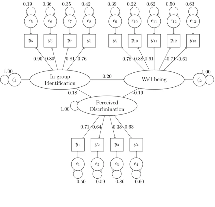
As an illustration, confidence bounds and fungible parameter contours are ob-tained from a published example in social psychology (Schmitt, Branscombe, Kobrynow-icz & Owen, 2002). The authors fit a latent variable (LV) mediation model to data ob-tained from a group of women (N = 220 ) where the effect of perceived discrimination against one’s in-group on psychological well-being was hypothesized to be mediated by in-group identification. Perceived discrimination was indicated by four measured vari-ables (MVs) - in-group disadvantage (y1) , out-group privilege (y2), prejudice across contexts (y3) and past experience with discrimination (y4). In-group identification was indicated by four MVs quantifying the extent of emotional attachment to one’s group - liking one’s group (y5), valuing one’s group (y6), having pride in one’s group (y7) and having positive experiences due to being a member of one’s group (y8). Fi-nally, psychological well-being was indicated by five MVs - life satisfaction (y9), self-esteem (y10), positive affect (y11), anxiety (y12) and depression (y13). To identify the model, all LVs were scaled according to their first indicators by fixing respective factor loadings to 1.0. Figure 1 is a path diagram of the model with standardized ML esti-mates.
Figure 1: Path Diagram for Schmitt et al. (2002) Mediation Model
5 6 7 8 9 10 11 12 13
0.19 0.36 0.35 0.42 0.39 0.22 0.62 0.50 0.63
y5 y6 y7 y8 y9 y10 y11 y12 y13
In-group
Identification Well-being
Perceived Discrimination
ζ1 ζ2
1.00 1.00
1.00
0.20
0.18 -0.19
0.90 0.80 0.81 0.76 0.78 0.88 0.61 -0.71 -0.61
y1 y2 y3 y4
1 2 3 4
0.71 0.64 0.38 0.63
1.7.1 Direct Effect (k = 1)
The ML estimate for the direct effect of perceived discrimination on well-being is ˆθf = −0.19 . In order to compute a 95% confidence interval for this focal parameter,
the perturbation applied to ˆF as defined in Equation 13 is χ20.95(1)/(220−1) = 0.0175 , and the profile likelihood-based confidence interval for this direct effect is (−0.389,−0.010) . As the confidence interval does not capture the value of θf = 0 , the direct effect of
perceived discrimination on well-being is statistically significant at p < .05 . Such a conclusion is consistent with Schmitt, et al. (2002) who would have obtained a stan-dard error of 0.092, and a Wald-type confidence interval of (−0.368,−0.008) . Note that the Wald-type confidence interval is different from the estimated likelihood-based confidence interval due to the former using a quadratic approximation of the likelihood function.
To compute fungible parameter values, the RMSEA perturbation of ˜ = 0.005 to model fit is specified, such that from Equations 6 and 7, ˆF∗ = 0.620 and Fp =
0.044 . In this example, the two fungible parameter values are (−0.533,0.097) . Since these two values are of different signs, the direct effect of perceived discrimination on well-being is not consistently negative under the minor perturbation introduced to model fit. These results suggest that the effect of perceived discrimination on well-being is sensitive to a perturbation of model fit. Hence, the robustness of this signif-icant direct effect is somewhat questionable, and the direct effect is said to be sen-sitive to a perturbation resulting in practically the same model fit as the ML solu-tion. Note that these fungible parameter values are larger in magnitude compared to the confidence bounds as the perturbation applied to the ML estimate for the former (Fp = 0.044 ) is larger than the latter (Fp = 0.0175 ).
0.071 . This is equivalent to perturbing the RMSEA by ˜ = 0.071−0.0687 = 0.002 , a value smaller than the specified perturbation of ˜ = 0.005 , which was used to compute the two fungible parameter values above. Alternatively, the perturbation associated with the fungible values translates to χ2
1−α(1) = (220−1)(0.578−0.576) = 9.672 , which
is associated with a 99.81% confidence interval along with α= 0.002 .
The above calculations show that confidence bounds may be translated to fgible parameter values and vice versa. However, the conversion of one measure of un-certainty to the other may not necessarily be meaningful. First, the fungible parameter values are numerically equivalent to constructing a 99.81% confidence interval. How-ever, the associated small error rate of α = 0.002 is not practically useful in making statistical inferences. Second, the 95% confidence interval is equivalent to a model per-turbation of ˜ = 0.002 . While this perturbation is smaller than the specified perturba-tion used to compute fungible parameter values, ˜ = 0.002 is practically no different from ˜ = 0.005 in terms of model fit. The small difference of 0.003 between these two perturbations of RMSEA was associated with fungible parameter values with different conclusions regarding θf = 0 , implying that the direct effect is sensitive to the
magni-tude of perturbation applied to model fit.
1.7.2 Indirect Effect (k= 2)
The effect of perceived discrimination on psychological well-being was hypothe-sized to be mediated by in-group identification, and the ML estimates for the effect of perceived discrimination on in-group identification and the effect of in-group identifica-tion on well-being are ˆθf = (0.18,0.20)0. To compute the 95% confidence bound for the
focal parameters, we apply a perturbation of χ2
0.95(2)/(220−1) = 0.0273 as defined in Equation 13. Recall that a perturbation of ˜= 0.005 or Fp = 0.044 is used to compute
the fungible parameter contour. Hence, it is expected that the latter has larger values than the former. Figure 2 depicts the simultaneous 95% confidence region (as blue col-ored crosses) and the fungible parameter contour (as red colcol-ored circles) based on the profile likelihood.
Figure 2: Profile Likelihood-Based Confidence Bounds and Fungible Contours for the Indirect Effect of Perceived Discrimination on Well-being.
−0.4 −0.2 0.0 0.2 0.4 0.6 0.8
−0.4 −0.2 0.0 0.2 0.4 0.6 0.8
Effect of Percevied Discrimination on In−group Identification
Eff
ect of In−group Identification on W
ell−being ● ● ● ● ● ● ● ● ● ● ● ● ● ● ● ● ● ● ● ● ● ● ● ● ● ● ● ● ● ● ● ● ● ● ● ● ● ● ● ● ● ● ● ● ● ● ● ● ● ● ● ● ● ● ● ● ●● ●● ● ●●●● ●●●●●●●●●●●●●●●●●●●● ●●●● ●● ●● ●● ●● ●● ● ● ● ● ML Estimate
95% Confidence Bound Fungible Parameter Contour
θf = (0,0)0, implying that the estimated effects are not simultaneously significant at
p < .05 . Additionally, the fungible parameter values take on all possible combinations
of positive and negative values for each of the effects, suggesting that the results are sensitive to a perturbation to model fit. Hence, the distinct information on parameter uncertainty, as depicted in the elliptical forms of Figure 2, implies that the mediation effect may not be interpreted vigorously.
It is noted that Schmitt et al. (2002) drew the opposite conclusion that the two effects are significant at p < .05 . However, there are at least two explanations for this inconsistency. First, Schmitt, et al. (2002) conducted their hypothesis tests using the Wald test. Although the two effects were statistically significant at p < .05 , the Wald-type confidence intervals were close to θf = (0,0)0; the intervals are (0.004,0.346) and
(0.042,0.352) for the effect of perceived discrimination on in-group identification and the effect of in-group identification on psychological well-being respectively. Addition-ally, the profile likelihood-based confidence regions reported here are, however, based on an LRT. While the Wald test and LRT are asymptotically equivalent, a sample of N = 220 may not be large enough for these two test results to converge. It is notewor-thy to mention here that the LRT is usually more reliable than the Wald test for small to mid-sized samples (Agresti, 2002).
param-eter estimates is accounted for. Therefore, the non-simultaneous Wald tests reported in Schmitt, et al. (2002) tended to be overpowered compared to a joint test associated with the confidence region in Figure 2.
As the fungible parameter values in Figure 2 take on all combinations of pos-itive and negative values, the sign of both effects may be reversed given a practically similar model fit to the optimal ML solution. Observe that the range of the fungible values for the effect of perceived discrimination on in-group identification is wider than the effect of in-group identification on well being; this suggests that the latter effect is relatively less sensitive to the former effect under a small perturbation to model fit. The two measures of uncertainty, computed from the estimated likelihood, suggest that the indirect effect of perceived discrimination on well-being should not be interpreted rigorously.
1.7.3 Summary and Extensions
Confidence regions may be translated to fungible parameter contours and vice-versa as demonstrated in the empirical illustration. However, the example showed that the resulting information gained from translating confidence regions into fungible pa-rameter contours may be of limited value. In particular, the equivalence of these es-timates was achieved at the expense of their interpretability, especially for confidence regions. However, it may not always be the case that the equivalence between confi-dence regions and fungible parameter values occur under unrealistic or substantively less meaningful conditions. In situations where these two kinds of parameter uncer-tainty are meaningful numerical translations of each other, they provide unique and useful information to the analyst.
Chapter 2
METHODS
There were three objectives of the project. The first two aims of establishing the analytical relationship between confidence regions and fungible parameter contours, and implementing computations to be based on the profile likelihood have been accom-plished. The remaining objective is to assesses how certain factors affect confidence regions and fungible parameter contours. These factors involve certain modelling condi-tions, the perturbation schemes used to construct fungible parameter contours, as well as whether computations are based on the empirical or profile likelihood. The following sections describe how each of these factors are examined in the simulation study.
2.1 Modelling Factors that May Impact Parameter Uncertainty
To better understand the nature of the two kinds of parameter uncertainty -confidence bounds and fungible parameter values - it is proposed that certain mod-elling factors which may influence them are examined. The three factors explored are sample size, overall model fit, and the magnitude of correlations among MVs. As this aspect of the project is exploratory, the following suggested hypotheses on how the three factors may affect the two kinds of parameter uncertainty differently are only working hypotheses based on informed speculation.
increas-ing sample size would lead to tighter confidence regions, reflectincreas-ing higher precision and lower sampling variability of the estimates. It is also expected that changes in sample size will not affect the size of fungible parameter contours. Stated differently, fungible parameter contours are expected to be independent of sample size. Yet with different sample sizes, fungible parameter values should not remain constant; instead these con-tours are expected to shift slightly from sample to sample, reflecting sampling variabil-ity. Note that the sampling variability expected to be reflected in fungible parameter values does not result from the effect of sample size, but the variation in the correla-tions among MVs across the different samples.
Second, from limited exploratory computations of fungible parameter values on published examples, an apparent tendency for the size of fungible parameter con-tours to be related to model fit has been observed. In particular, larger fungible pa-rameter contours were found to be associated with less well-fitting models. Alterna-tively, smaller fungible parameter contours were found to be observed when the fit of the model was good. It is plausible that the likelihood surface would be less peaked when model fit is not extremely good (Michael Browne, personal communication March 2011). A basis for conjecture regarding this phenomenon is that when model fit is not very good, the sample discrepancy function values based on ML and GLS estimation can differ substantially (Browne, MacCallum & Kim, 2002), possibly implying a flatter likelihood surface. Alternatively, when the sample discrepancy function values based on ML and GLS estimation coincide in the context of good model fit, the likelihood function may tend to be more peaked. With a more peaked likelihood surface, fungible parameter contours as well as confidence regions are anticipated to be tighter compared to a flatter likelihood surface.
words, fewer models can fit well to data structures with large correlations among MVs compared to data structures with small correlations among MVs. This limited number of models in data structures with larger correlations translates to more peaked likeli-hood surfaces which are expected to be associated with tighter confidence bounds and fungible parameter contours. Stated differently, higher correlations are expected to be associated with fungible parameter values that provide data descriptions that are tol-erably different from the ML solution. Likewise, holding sample size constant, larger correlations are expected to be associated with more precise confidence regions.
The following section describes the exploratory simulation study used to assess the effect of sample size, model fit and the magnitude of correlations among MVs on the size of confidence regions and fungible parameter contours. Additionally, the as-sertion that parameter sensitivity (or parameter fungibility) is a property of the model (Green, 1977) and not the sample is empirically examined.
2.1.1 Population Generating Models
The empirical illustration based on Schmitt, et al. (2002) will serve as the blueprint to generating data for the proposed exploratory simulation study. Recall that there
were 13 MVs and 3 LVs involved in this model of LV mediation (see Figure 1). The general SEM model in covariance structure form is expressed as
Σ=Λ(I−B)Φ(I−B)0Λ0+Ψ (22)
In particular, the population generating model has the following specified matrices: Λ=
0.8073 0 0
0.8102 0 0
0.8047 0 0
0.8059 0 0
0 0.8086 0
0 0.8072 0
0 0.8038 0
0 0.8017 0
0 0 0.8007
0 0 0.8043
0 0 0.8004
0 0 0.8081
0 0 0.8055
and Φ=
1.0 0 1.0
0 0 1.0
.
The values for Ψ and B will be introduced in the following section where different magnitudes of correlations between the MVs are specified. Note that these popula-tion values for Λ and Ψ are based on the estimated values reported in Schmitt et al. (2002).
2.1.1.1 Magnitude of Correlations
more weight on structural paths. The study will fully cross these two methods for ma-nipulating the correlations among MVs.
The size of unique variances indirectly affects correlations between MVs. The variance of each MV is attributable to three sources of variation - common variance, specific variance, and error variance. The common variance is attributable to the com-mon factor or LV, the specific variance represents systematic factors affecting a given MV and the error variance represents random error of measurement or unreliability. Hence, reliable variance in any given MV is made up of common and specific variances. Unique variance is made up of the sum of specific and error variances. Small unique variances indirectly translate to larger correlations between MVs as they reflect ac-curacy of measurement associated with increased power to reject false models. Addi-tionally, when MVs have smaller unique variances, effect sizes tend to be larger and power of the LRT will be high (Browne, MacCallum & Kim, 2002), implying tighter confidence regions due to a more peaked likelihood surface. As fungible parameter con-tours are also based on the peakedness of the likelihood surface, they are expected to be tighter when unique variances of MVs are small. Large measurement errors take on values close to Ψp,p = 0.50 where p = 1,· · · ,13 . These unique variances are not
ex-actly 0.50 , but randomly vary very slightly from one another to avoid equivalent pop-ulation parameter values. In addition, these values were chosen to follow the unique variances observed in Schmitt, et al. (2002) where 0.19≤ Ψp,p ≤ 0.86 . Small
measure-ment errors similarly take on values close to Ψp,p = 0.10 .
effect sizes are specified using
B =
0 0 0
0.2076 0 0
−0.1989 0.2015 0
,
which reflects the values observed by Schmitt, et al. (2002) where β2,1 = 0.17 , β3,1 =
−0.18 and β3,2 = 0.19 . In contrast, large effect sizes are specified using
B =
0 0 0
0.6076 0 0
−0.5989 0.6015 0
.
With the two different specifications of Ψ and the two different specifications of B, there are four possible population covariance matrices. Let the subscripts ΨL
and ΨH denote low and high correlations among MVs due to controlling the size of
unique variances. Similarly, let the subscripts BL and BH denote low and high
corre-lations resulting from manipulating the size of the structural effects respectively. It is emphasized that L and H refer to low and high correlations among MVs due to ma-nipulating Ψ and B, and not the values within these two matrices themselves. Hence, ΣΨLBL refers to the population covariance matrix based on large unique variances and
small structural effect sizes. It follows that ΣΨHBL refers to the population covariance
matrix defined by small unique variances and small structural effect sizes, ΣΨLBH is
the population covariance matrix due to large unique variances and large effect sizes and ΣΨHBH is the population covariance matrix derived from small unique variances
and large structural effects. Let PΨLBL, PΨHBL, PΨLBH and PΨHBH denote their
commensurate population correlation matrices.
variances and small effect sizes is
ΣΨLBL and PΨLBL =
1.15 0.57 0.56 0.56 0.12 0.12 0.12 0.12 0.13 0.13 0.13 0.13 0.13
0.65 1.16 0.56 0.56 0.12 0.12 0.12 0.12 0.13 0.13 0.13 0.13 0.13
0.65 0.65 1.16 0.56 0.12 0.12 0.11 0.11 0.13 0.13 0.13 0.13 0.13
0.65 0.65 0.65 1.16 0.12 0.12 0.11 0.11 0.13 0.13 0.13 0.13 0.13
0.14 0.14 0.14 0.14 1.18 0.57 0.57 0.57 0.14 0.14 0.14 0.14 0.14
0.14 0.14 0.13 0.14 0.68 1.18 0.57 0.57 0.14 0.14 0.14 0.14 0.14
0.13 0.14 0.13 0.13 0.68 0.68 1.18 0.57 0.14 0.14 0.14 0.14 0.14
0.13 0.13 0.13 0.13 0.68 0.68 0.67 1.18 0.14 0.14 0.14 0.14 0.14
0.16 0.16 0.16 0.16 0.16 0.16 0.16 0.16 1.21 0.58 0.58 0.59 0.59
0.16 0.16 0.16 0.16 0.16 0.16 0.16 0.16 0.71 1.22 0.58 0.58 0.59
0.16 0.16 0.16 0.16 0.16 0.16 0.16 0.16 0.70 0.71 1.21 0.58 0.58
0.16 0.16 0.16 0.16 0.16 0.16 0.16 0.16 0.71 0.71 0.71 1.22 0.59
0.16 0.16 0.16 0.16 0.16 0.16 0.16 0.16 0.71 0.71 0.71 0.72 1.21
where the covariances among the MVs are presented in the lower triangular matrix, the variances are bold in the diagonal of the matrix, and the correlations are italicized in the upper triangular matrix. Note that ΣΨLBL and PΨLBL have values based on
Schmitt et al.’s (2002) empirical study. The remaining three population covariance matrices (ΣΨHBL, ΣΨLBH, and ΣΨHBH) as well as correlation matrices (PΨHBL,
PΨLBH, and PΨHBH) are presented in Appendix A.
2.1.1.2 Model Fit
do not appear to follow models which hold exactly in the samples (Tucker, Koopman & Linn, 1969). Introducing noise to the regularity of the population generating model reflects any variety of unsystematic or unknown aspects of the process which gave rise to the observed data. Two levels of model fit - good and poor - are predetermined. For good model fit, a population RMSEA value of = 0.03 is used. Alternatively, for poor model fit, a population RMSEA value of = 0.09 is specified.
To illustrate, the population covariance and correlation matrix associated with large unique variances and small effect sizes for good model fit is
ΣΨLBLG and PΨLBLG =
1.15 0.58 0.55 0.56 0.12 0.11 0.14 0.12 0.13 0.13 0.15 0.14 0.15
0.67 1.16 0.56 0.55 0.13 0.13 0.11 0.10 0.12 0.13 0.14 0.12 0.14
0.63 0.65 1.16 0.58 0.11 0.11 0.08 0.10 0.11 0.12 0.14 0.10 0.11
0.64 0.64 0.67 1.16 0.13 0.10 0.11 0.15 0.14 0.15 0.16 0.13 0.14
0.14 0.15 0.13 0.16 1.18 0.59 0.58 0.56 0.12 0.17 0.18 0.12 0.14
0.13 0.15 0.13 0.11 0.69 1.18 0.56 0.57 0.11 0.13 0.14 0.12 0.13
0.16 0.13 0.10 0.13 0.68 0.66 1.18 0.58 0.13 0.13 0.12 0.11 0.11
0.14 0.12 0.12 0.17 0.66 0.68 0.69 1.18 0.14 0.15 0.16 0.13 0.18
0.15 0.14 0.13 0.17 0.14 0.13 0.16 0.16 1.21 0.57 0.59 0.60 0.57
0.16 0.15 0.15 0.18 0.20 0.16 0.15 0.18 0.70 1.22 0.59 0.57 0.60
0.17 0.16 0.17 0.19 0.21 0.17 0.14 0.19 0.71 0.71 1.21 0.58 0.57
0.16 0.15 0.12 0.16 0.15 0.15 0.13 0.15 0.73 0.70 0.70 1.22 0.59
0.18 0.16 0.13 0.17 0.17 0.16 0.14 0.21 0.70 0.73 0.70 0.72 1.21
2.1.1.3 Sample Size
Two sample sizes were chosen to cover the range of designs that are used in applied psychological research. The moderate sample size is N = 200 and the large sample size is N = 1000 . The large difference in these values is meant to cover a broad range of sample sizes in addition to amplifying the effect of sample size on confidence bounds and fungible parameter values.
2.1.2 Study Conditions
From the model specifications laid out, there are four derived population co-variances constructed with (a) large unique co-variances and small structural effects ΣΨLBL,
(b) small unique variances and small structural effects ΣΨHBL, (c) large unique
vari-ances and large structural effects ΣΨLBH and (d) small unique variances and large
structural effects ΣΨHBH. To be explicit, let the subscript 0 denote covariance
ma-trices which hold exactly in the population. For example, ΣΨLBL0 is the population
covariance matrix based on large unique variances and small structural effects which holds exactly in the population.
Noise may then be added to these four population covariance matrices, which hold exactly, via the Cudeck and Browne (1992) method. Let the subscripts G and P denote good and poor model fit respectively. Therefore, ΣΨLBLG is the population
covariance matrix based on large unique variances, small structural effects and good model fit, ΣΨLBLP is the population covariance matrix based on large unique
vari-ances, small structural effects and poor model fit, and so on. By adding two levels of model error to the four population covariances, there are a total of 4×3 = 12 popula-tion covariance matrices (see Appendices A and B).
as computing profile likelihood-based confidence regions and fungible parameter con-tours is computationally intensive. Additionally, we are not focused on the repeated sampling properties of likelihood-based confidence intervals and fungible parameter contours. Let the subscripts N200 and N1000 denote the moderate and large sample sizes. Following the established notation, let SΨLBLGN200 denote the sample covariance
matrix constructed with large unique variances, small structural effects, good model fit and moderate sample size; likewise, SΨLBLGN1000 is the sample covariance matrix
based on large unique variances, small structural effects, good model fit and large sam-ple size, and so forth.
In summary, there are a total of 12 proposed population conditions where only fungible parameter values can be obtained. Additionally, we will compute both likelihood-based confidence bounds and fungible parameter contours for the 24 sample conditions. Of interest, is the indirect effect of the LV mediation concerning the focal parameters of θf = (β2,1, β3,2)0. Hence, the study has a total of 24 + 12 = 36 conditions. Ta-ble 1 summarizes the 36 cells associated with the proposed design. Estimation will be carried out using R (R Development Core Team, 2010).
2.2 Perturbation Schemes
Confidence regions and fungible parameter contours may be constructed from the general perturbation framework as laid out in Equations 10 and 13. The “pertur-bation” applied to obtain confidence regions is derived directly from the LRT, and is an objective function of sample size and the quantiles of the χ2 distribution (see Equation 13). Following convention, we will construct 95% confidence regions where α= 0.05 .
In contrast to confidence regions, the choice of perturbations to be used to compute fungible parameter contours is a subjective one. As a general principle, per-turbations should be very small such that the change in model fit is practically no dif-ferent from the fit of the optimal solution; the constructed fungible parameter contour will therefore contain alternative exchangeable parameter values that describe the data almost as well as the optimal solution in terms of model fit. As suggested by MacCal-lum, Browne and Lee (2009), and consistent with the perturbation scheme used in our empirical demonstration, we continue to use the perturbation based on RMSEA for all study cells. Specifically, the RMSEA perturbation is chosen to be ˜ = 0.005 , corre-sponding to a practically insignificant difference in model fit.
Additionally we implemented a perturbation directly to the sample discrep-ancy function value ˆF to compute fungible parameter contours. In particular, a small percentage of ˆF was used as the alternative perturbation scheme. For a subset of the study cells, a perturbation of % ˆF = 5% or ˆF∗ = 1.05 ˆF will be used to compute fungible parameter contours. These two perturbation schemes were applied to the con-ditions of large unique variances and small structural effects (ΨLBL) as well as small
unique variances and large structural effects (ΨHBH) to obtain two distinct sets of
2.3 Profile and Empirical Likelihood-Based Computation
Estimates based on the empirical likelihood, as implemented by MacCallum, Browne and Lee (2009), have the advantage of computational efficiency over estimates based on the profile likelihood. In a multi-parameter context, where interest is in a se-lected set of focal parameters θf, the estimated likelihood makes use of a single ML
solution to take account of the nuisance parameters θn. Here, the nuisance
parame-ters take on values of ˆθn which are the estimates of the nuisance parameters obtained
jointly with the focal parameters, ˆθf. In other words, the estimated likelihood does
not re-compute θn or ˜θn in the search for fungible parameter values or confidence
bounds (see Equations 20 and 21). However, confidence bounds and fungible parameter contours based on the empirical likelihood may be biased downward. Stated differently, confidence bounds computed from the estimated likelihood, compared to the profile likelihood, may communicate overly optimistic precision (Pawitan, 2001). Likewise, fungible parameter contours obtained from the estimated likelihood may be tighter than contours obtained from the profile likelihood. By substituting ˆθn for ˜θn, the
es-timated likelihood does not take account of the uncertainty of the nuisance parameters and the correlations among the nuisance and focal parameters, causing potential bias in estimates.
The advantage of obtaining less biased estimates from the profile likelihood outweighs the computational burden of having to re-compute ˜θn for every point on the