Marriage, divorce and economic
activity in the US: 1960–2008
Hamid Baghestani
a,*
and Michael Malcolm
b aDepartment of Economics, School of Business and Management, American University of Sharjah, Sharjah, 26666 UAE
b
Department of Economics, West Chester University of Pennsylvania, West Chester, PA 19383, USA
We utilize a time-series model to examine the interrelationship between marriage and divorce and their connections with macroeconomic conditions for the period 1960 to 2008. Ourfindings suggest that marriage and divorce are pro-cyclical, although macroeconomic conditions affect divorce only when the economy is underperforming. Marriage is pro-cyclical in all circumstances. Further, bidirec-tional causation exists, with marriage (divorce) affected by lagged rates of divorce (marriage).
Keywords: demographics; marital formation; GDP gap; unemployment gap;
causality
JEL Classification: J12; C32
I. Introduction
Individual choices related to household and family structure are known to be associated with aggregate economic conditions. Becker (1981) observed that volun-tary marriages must raise the expected utility of both spouses above what it would have been if they had remained single. Economies of scale, income gains from specialization and the prospect of investing in high-quality children are among the most important quan-tifiable welfare improvements, and all are affected by macroeconomic conditions. Conversely, divorces occur when one spouse determines that his or her utility is higher outside marriage, and this comparison is also affected by the economy at large.
Most existing research estimates the magnitude of these effects by using household-level data. Time-series studies that relate marriage and divorce to macroeco-nomic aggregates are sparse. We specify a time-series model to better understand the interrelationship between marriage and divorce and their connections with
macroeconomic conditions for the period 1960–2008. We use both GDP and unemployment gaps, which we argue are more informative indicators than the unem-ployment rate commonly used in the literature. Wefind that marriage displays pro-cyclical behaviour, with the responsiveness to the unemployment gap being larger when the economy is underperforming. Divorce is pro-cyclical only when the economy is underperforming; widening of the gap inversely affects divorce. Finally, the relationship between marriage and divorce exhibits bidirectional causality. Section II presents a literature review. Section III reports the empirical results. Section IV interprets the results.
II. Related Literature
While the economic climate can affect incentives to marry and divorce, the direction of these effects is theoretically ambiguous. Ekert-Jaffe and Solaz (2001) and Guitierrez-Domenech (2008) find that the formation of initial
*Corresponding author. E-mail:[email protected]
Vol. 21, No. 8, 528–532, http://dx.doi.org/10.1080/13504851.2013.872753
marriages is positively associated with good economic circumstances. Jensen and Smith (1990) and Eliason (2012)find that bad economic circumstances leading to job loss induce divorce. As such, these studies suggest that improvements in economic conditions increase marriages and reduce divorce.
However, bad economic circumstances can elevate the importance of economies of scale from cost-sharing in multi-person households. Harknett and Schneider (2012)
find that economic distress reduces the probability of divorce. Shore (2010) argues that the risk-sharing benefits of marriage are more important during bad economic times.
To the extent that cyclical fluctuations affect men and women differently, a change in economic conditions can disrupt bargaining power within marriages, which has implications for the divorce rate (Kesselring and Bremmer, 2006). But the direction is uncertain. Clark and Summers (1981) argue that cyclicalfluctuations affect women more strongly than men in all age groups. Elsby
et al. (2010)find the opposite with respect to the recent recession.
Further, in newer theoretical models, the marriage– divorce relationship features bidirectional causality. Evaluation of the utility from marrying versus remaining single depends on the probability of divorce, which in turn depends on howfluid the remarriage market is. Each feeds back to the other, possibly with a time lag (Chiappori
et al.,2008).
Among previous time-series studies, South (1985)finds that increases in unemployment are associated with higher divorce rates, while Schaller (2013)finds that both mar-riage and divorce are pro-cyclical with respect to employment outcomes. There are a few important innova-tions in our article. First, wefind that the level of respon-siveness is different when the economy is overperforming versus underperforming. Second, our model allows for bidirectional causality between marriage and divorce. Third, wefind that the GDP gap and the unemployment gap are more informative indicators than the unemploy-ment rate.
III. Data and Empirical Results
The annual data on the total marriages and divorces per 1000 population come from various issues of the National Vital Statistics Report, published by the National Center for Health Statistics up to 2008. The unemployment gap is the actual (civilian) unemployment rate minus the natural unemployment rate. The real GDP gap is 100 times the difference between the logarithm of actual GDP and the logarithm of potential GDP. The data on economic vari-ables are available on the Federal Reserve Bank of St. Louis website.
Both marriage and divorce rates (plotted inFig. 1 for the period 1960 to 2008) display strong quadratic trends. According to our unit root test results, the de-trended marriage and divorce series, the unemployment rate, unemployment gap and real GDP gap are all stationary around a constant. As such, we specify the following general model:
Mt¼a1þ X7
i¼1
b1iMtiþ X7
j¼0 b2jVtj
þb3D1jUtgapj þb4ð1D1ÞU gap t
j j
þb5D2jYtgapj þb6ð1D2ÞY gap t
j j þu1t
(1)
Vt¼a2þ X7
i¼1
c1iVtiþ X7
j¼0 c2jMtj
þc3D1jUtgapj þc4ð1D1ÞjU gap t j þc5D2jYtgapj þc6ð1D2ÞY
gap t
j j þu2t
(2)
whereMtandVtare, respectively, the de-trended marriage
and divorce rates. jUtgapj is the unemployment gap (in absolute value), andD1is a dummy (=1 whenUtgap> 0, and = 0 whenUtgap<0). Y
gap t
j jis the GDP gap (in absolute value), andD2is a dummy (=1 whenYtgap<0, and = 0 when Ytgap> 0). Note thatD1U
gap t
j jand D2jYtgapj corre-spond to the period when the economy is underperform-ing, and 1ð D1ÞjUtgapjand 1ð D2ÞY
gap t
j jcorrespond to the period when the economy is overperforming.
11 5.5 5.0 4.5 4.0 3.5 3.0 2.5 –2.0 –1.5 Marriage rate Divorce rate 10 9 8 7 6
1960 1965 1970 1975 1980 1985 1990 1995 2000 2005 1960 1965 1970 1975 1980 1985 1990 1995 2000 2005
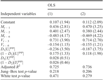
Equation 1 is initially estimated using OLS for 1960– 2008. Excluding the highly insignificant variables, the equation is then re-estimated, with the results reported in column 1 ofTable 1. As seen, the parameter estimates on both D2jYtgapj and 1ð D2ÞY
gap t
j j are not significantly different from zero. Excluding these variables, we have re-estimated the equation with the results reported in column 2. These estimates pass a series of diagnostic tests. For instance, the Ljung–Box test and the White
test results point to the absence of autocorrelation and heteroscedasticity in the error term, and the cusum of squares test results inFig. 2confirm that the equation is stable in terms of parameters. The parameter estimates on bothD1jUtgapjand 1ð D1ÞU
gap t
j jare significant, with the signs suggesting that marriage is pro-cyclical. However, the parameter estimate onD1jUtgapj, 0.187, is larger than the parameter estimate on 1ð D1ÞjUtgapj, 0.118, indicat-ing that marriage is more responsive to the gap when the economy is underperforming.1Further, the marriage rate, while contemporaneously independent of divorce, is affected by the lagged divorce rates.
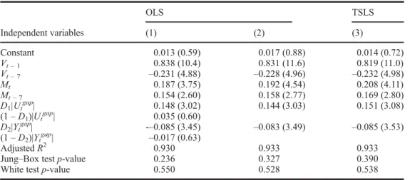
Next, Equation 2 is initially estimated using OLS. Excluding the highly insignificant variables, the equation is then re-estimated, with the results reported in column 1
of Table 2. As seen, the parameter estimates on both
1D1
ð ÞjUtgapjand 1ð D2ÞY gap t
j j are not significantly different from zero. Excluding these variables, we have re-estimated the equation with the results reported in column 2. The corresponding two-stage least squares (TSLS) estimates, which purge the simultaneous bias, are reported in column 3.2As seen, the TSLS estimates are very similar to the OLS estimates in column 2 and pass a series of diagnostic tests. For instance, the Ljung-Box test and the White test results point to the absence of autocorrelation and heteroscedasticity in the error term, and the cusum of squares test results in Fig. 2confirm that the model is stable in terms of parameters. The para-meter estimates on bothD1jUtgapjand D2Y
gap t
j jare sig-nificant, with the signs suggesting that divorce is pro-cyclical when the economy is underperforming; that is, widening of the gap inversely affects divorce. However, divorce does not respond to the gap when the economy is overperforming. Finally, divorce is contemporaneously Table 1. Marriage rate equation estimates (dependent
variable =Mt)
OLS
Independent variables (1) (2)
Constant 0.107 (1.94) 0.112 (2.09) Mt–1 0.436 (2.81) 0.470 (3.25)
Mt–2 0.401 (2.47) 0.380 (2.44)
Mt–6 –0.483 (4.17) –0.469 (4.22)
Vt–3 0.731 (3.90) 0.714 (2.70)
Vt–6 –0.154 (1.15) –0.155 (1.21)
D1|Utgap| –0.236 (3.50) –0.187 (3.75)
(1–D1)|Utgap| 0.175 (1.33) 0.118 (1.98)
D2|Yt gap
| 0.028 (0.51)
(1–D2)|Yt gap
| 0.026 (0.46)
AdjustedR2 0.725 0.736
Jung–Box testp-value 0.218 0.206 White testp-value 0.471 0.279
Notes:MtandVtare, respectively, the de-trended marriage rate
and divorce rate.jUtgapjis the unemployment gap (in absolute value), andD1is a dummy (=1 whenUtgap> 0, and = 0 when Utgap<0). |Ygapt| is the GDP gap (in absolute value), andD2is a
dummy (=1 whenYtgap<0, and = 0 whenYtgap> 0). Absolute t-ratios are in parentheses. The Ljung–Box test examines the null hypothesis of no autocorrelation problem up to the 12th order.
1.4
1.2 The marriage rate equation Cusum of squares; 5% significance
The divorce rate equation Cusum of squares; 5% significance 1.0
0.8 0.6 0.4 0.2 0.0 –0.2 –0.4
1.4 1.2 1.0 0.8 0.6 0.4 0.2 0.0 –0.2 –0.4
76 78 80 82 84 86 88 90 92 94 96 98 00 02 04 06 08 76 78 80 82 84 86 88 90 92 94 96 98 00 02 04 06 08
Fig. 2. Cusum of squares parameter stability test results
1
We have re-estimated the marriage equation in column 2 with the unemployment rate included along with D1jUtgapj and 1D1
ð ÞjUtgapj. Our results indicate that the parameter estimate on the unemployment rate (=0.222, with ap-value of 0.345) is insignificant. The parameter estimates on bothD1jUtgapjand 1ð D1ÞjUtgapj, however, remain significant.
2
determined by marriage and also is affected by the lagged marriage rates.
IV. Interpretation and Conclusions
Consistent with theory, both marriage and divorce are pro-cyclical when the economy is underperforming. For mar-riage, this effect is captured by a widening of the unem-ployment gap; for divorce, the unemunem-ployment gap and the GDP gap contain independent information. An important factor in the decision to marry is the potential for eco-nomic gains. A bad economy reduces the potential for these gains. However, for couples who are already mar-ried, an improvement in economic conditions increases the potential utility from separation. This effect is espe-cially strong for women, who initiate most divorces (Brinig and Allen,2000).
The effect of the economic climate on divorce is active
onlywhen the economy is underperforming. This
ampli-fies earlierfindings that economic distress stabilizes exist-ing marriages. A worsenexist-ing economy makes it difficult to divorce, because divorce dissolves the economies of scale and the risk sharing that characterize marriage. By con-trast, the formation of new marriages is pro-cyclical regardless of whether the economy is overperforming or underperforming. This follows the literature that the decision to marry is a calculated consideration of expected gains from marriage,3 while the relationship between divorce and the economy is specific to the economic stresses associated with an underperforming economy.
As for the bidirectional causality between marriage and divorce, the cumulative effect of lagged increases in one is an increase in the other. This follows newer theoretical
models which treat the process as dynamic (Chiappori
et al., 2008). An increase in the divorce rate feeds back to higher marriage rates by increasing remarriage. This improvement in remarriage prospects increases utility out-side of marriage, which in turn endogenously increases the divorce rate. Consistent with this approach, wefind the effect of divorce rates on subsequent marriage rates is lagged, while the effect of changes in marriage rates on divorce rates is both lagged and contemporaneous.
Acknowledgement
We thank Todd Sandler for helpful feedback.
References
Alm, J. and Whittington, L. A. (1995) Does the income tax affect marital decisions?,National Tax Journal,48, 565–72. Becker, G. S. (1981) A Treatise on the Family, Harvard
University Press, Cambridge.
Brinig, M. F. and Allen, D. W. (2000)‘These boots are made for walking’: why most divorcefilers are women,American Law and Economics Review,2, 126–69.
Chiappori, P. A., Iyigun, M. and Weiss, Y. (2008) An assignment model with divorce and remarriage. IZA Discussion Paper No. 3892. Available at http://ssrn.com/abstract=1318851 (accessed 23 December 2013).
Clark, K. B. and Summers, L. H. (1981) Demographic differ-ences in cyclical employment variation,Journal of Human Resources,16, 61–79.
Ekert-Jaffe, O. and Solaz, A. (2001) Unemployment, marriage, and cohabitation in France,Journal of Socio-Economics,
30, 75–98.
Eliason, M. (2012) Lost jobs, broken marriages, Journal of Population Economics,25, 1–33.
Table 2. Divorce rate equation estimates (dependent variable =Vt)
OLS TSLS
Independent variables (1) (2) (3)
Constant 0.013 (0.59) 0.017 (0.88) 0.014 (0.72)
Vt–1 0.838 (10.4) 0.831 (11.6) 0.819 (11.0)
Vt–7 –0.231 (4.88) –0.228 (4.96) –0.232 (4.98)
Mt 0.187 (3.75) 0.192 (4.54) 0.208 (4.11)
Mt–7 0.154 (2.60) 0.158 (2.77) 0.169 (2.80)
D1|Utgap| 0.148 (3.02) 0.144 (3.03) 0.151 (3.08)
(1–D1)|Utgap| 0.035 (0.60)
D2|Ytgap| -–0.085 (3.45) –0.083 (3.49) –0.085 (3.53)
(1–D2)|Ytgap| –0.017 (0.63)
AdjustedR2 0.930 0.933 0.933
Jung–Box testp-value 0.236 0.327 0.390
White testp-value 0.550 0.528 0.538
Notes: See the notes inTable 1.
3
Elsby, M. W., Hobijn, B. and Sahin, A. (2010) The labor market in the Great Recession. NBER Working Paper No. 15979. Available athttp://www.nber.org/papers/w15979(accessed 23 December 2013).
Gutiérrez-Domènech, M. (2008) The impact of the labour mar-ket on the timing of marriage and births in Spain,Journal of Population Economics,21, 83–110.
Harknett, K. and Schneider, D. (2012) Is a bad economy good for marriage? The relationship between macroeconomic conditions and marital stability from 1998–2009, National Poverty Center Working Paper Series #12-06. Available at http://npc.umich.edu/publications/u/2012-06%20NPC% 20Working%20Paper.pdf(accessed 23 December 2013). Jensen, P. and Smith, N. (1990) Unemployment and marital
dissolution,Journal of Population Economics,3, 215–29.
Kesselring, R. G. and Bremmer, D. (2006) Female income and the divorce decision: evidence from micro data,Applied Economics,38, 1605–16.
Oreffice, S. and Quintana-Domeque, C. (2010) Anthropometry and socioeconomics among couples: evidence in the United States,Economics & Human Biology,8, 373–84. Schaller, J. (2013) For richer, if not for poorer? Marriage and
divorce over the business cycle, Journal of Population Economics,26, 1007–33.
Shore, S. H. (2010) For better, for worse: intrahousehold risk-sharing over the business cycle,The Review of Economics and Statistics,92, 536–48.