TECHNICAL UNIVERSITY OF CLUJ-NAPOCA
ACTA TECHNICA NAPOCENSIS
Series: Applied Mathematics, Mechanics, and Engineering Vol. 60, Issue III, September, 2017
GENERALIZED FORCES IN ANALYTICAL DYNAMICS OF SYSTEMS
Iuliu NEGREAN
Abstract: In the case of the multibody systems (MBS), as example the mechanical robot structure, and in accordance with differential principles typical to analytical dynamics of systems, the study of dynamical behavior is based on the generalized forces. They are developed in the direct connection with the generalized variables, also named independent parameters corresponding to holonomic mechanical systems. But, mechanically, the generalized forces are due to: driving sources of the mechanical motion, gravitational forces, manipulating loads, as well as complex frictions from physical links between the kinetic ensembles belonging to MBS. The expressions of definition of the generalized forces contain on the one hand kinematical parameters corresponding to absolute motions, on the other hand the mass properties. The last are highlighted by mass and position of the mass center, inertial tensors and pseudoinertial tensors. By means of the especially researches of the author, in this paper new formulations concerning the kinematical parameters, generalized forces and dynamics equations of the current and sudden motions will be presented. The dynamics study will be also contain acceleration energy and its time derivatives according to differential equations of higher order, typically to analytical dynamics of systems.
Key words: analytical dynamics, mechanics, generalized forces, dynamics equations, robotics.
1. INTRODUCTION
In the case of the multibody systems (MBS), as example the mechanical robot structure, see Fig.1, and according with differential principles answerable to analytical dynamics of systems, the study of dynamical behavior is based on, among others, the generalized forces [3] – [15]. They are mechanically developed in the direct connection with the generalized variables, also named independent parameters (d.o.f.) which they univocally characterize the absolute motion for holonomic mechanical systems. But, mechanically, the generalized forces are due to: driving sources of the mechanical motion, gravitational forces, manipulating loads, as well as complex frictions from physical links between the kinetic ensembles belonging to MBS (for example see Fig.1). In the same time, the expressions of definition for the generalized dynamics forces contain the both kinematical parameters corresponding to absolute motions, geometrical features, and the mass properties. The last are highlighted by mass and position of the mass center, as well as inertial tensors and pseudoinertial tensors [4], [5], [7], [8] and [14].
On the basis of the especially researches of the author, in the four sections of this paper new formulations will be presented. So, the first section is devoted to the kinematical parameters typical to MBS (mechanical robot structures) with current and sudden motions. Second and third sections of the paper highlight, by means of transfer matrices, the generalized gravitational, manipulating and inertia forces, as well as the generalized friction forces. In the fourth section dynamics equations with acceleration energies and their time derivatives according to [9] - [14] are developed. They are typical to the analytical dynamics of systems with sudden motions.
Fig.1 Mechanical Robot Structure (MBS)
0 y 1 y
2 y 3 y
5 4 y y ≡
0 x
1 x
2 x 3 x
5 4 x x ≡
0 z 1 z
3 z
2 z
5 4 z z ≡
n
s a
0 l
1 l
2 l
3 l
2. KINEMATICS PARAMETERS OF MBS
The kinematical and dynamical study from this paper [4], [5], [7] is oriented on mechanical structure with opened kinematical chain, where
the kinetic ensembles i= →1 n are physically
linked by driving joints of fifth order. (Example mechanical robot structure sees Fig.1).
Fig.2 Sequence of Kinetic Ensembles
This is characterized by
(
n d.o.f .)
, according to:( )0
( )
( )
Ti
; t q t ; i 1 n
θ ≠θ θ = = → , (1)
where q ti
( )
is the generalized coordinate fromevery driving axis. But, considering the current and sudden motions the generalized variables of higher order are developed as follows:
( )
( )
( )
( )
( )
( )
( )
( )
( )( )
m
m
i i i i
t ; t ; t ; ; t
q t ; q t ; q t ; ; q t
i 1 n, m 1
θ θ θ θ
=
=
= → ≥
& && L
& && L
, (2)
and
( )
m represents the time deriving order. Themain objective of this section consists in the establishment of the absolute angular and linear velocities and accelerations for every kinetic ensemble from MBS. Unlike the classical approaches [3] – [5], [7] in the following a few formulations based on the time derivatives of the locating matrices will be developed.
So, in the Fig.2 a sequence of two kinetic ensembles belonging to MBS is subjected to kinematical study. According to [5] – [7], the locating matrices are the following:
[ ]
( )
[ ]
( )
[ ]
( )
[ ]
( )
( )
[ ]
( )
[ ]
0 0 i 1
i i i
0
i i
0 i 1
i 1 ii 1
i 1 i
T t T t T t
R t p t
0 0 0 1
R t R p p
0 0 0 1
−
−
− −
−
= ⋅ =
=
⋅ +
=
, (3)
They define the locating (position – orientation) of the moving frame
{ }
i versus{ }
0 . The components with the same significance are written below thus:[ ]( ) [ ]( ) ( )
= − −
−
1 0
0 0
t p t R t
T i 01 i 1
0 1
i , (4)
[ ]( ) [ ]
= − − −
−
1 0 0 0
p R t
T i 1i i 1 ii 1
1 i
i , (5)
The matrix components from (3) – (5) are:
[ ] ii 1
(
i i( ) i)
1 i
i R =R − ⋅R k ;q t ⋅∆
− , (6)
( )
(
)
( )i 1 i i i 0
1 ii 1 i 1 ii 1
i p p 1 q t − k
− − −
− = + −∆ ⋅ ⋅ , (7)
[ ]
R( )
t i 01[ ]
R( )
t i 1i[ ]
R 0i
−
− ⋅
= , (8)
( )
( )
( )
( )
[ ]
i 1 ii 10 1 i 1 i 1 ii 1 i
i t p t p t p t R p
p = − + − = − +− ⋅− − , (9)
[
] [
]
{
}
i 1, i R ; 0, i T
∆ = = = ; (10)
The symbol (10) shows the driving joint type. On matrix (3) is applied the first time derivative:
( )
( )
( )
( )
[ ]
( )
[ ]
( )
( )
0 0
i i
i
0 i 1 0 i 1
i i 1
i 1 i
R t p t
T t
0 0 0 0
T t − T t − T t − T t
−
= =
= ⋅ + ⋅
& & &
& &
. (11)
The matrix components from right member are:
( )
[ ]
( )[ ]
0 i 1
i i 1
0 i 1 0
i 1
i 1 i i 1
i
i 1 i 1
T t T t
R R p R p
0 0 0 1
− −
−
−
− −
− −
⋅ =
⋅ + ⋅
=
&
&
& & ; (12)
[ ]( ) ( )
[ ]( ) ( )
(
)
[ ]( ) ( )
(
)
( )i 1 0
i 1 i
i 1
0 i 1
i i i i 1 i 1
i 1 i
i 1 0 i i i i i i i 1
T t T t
R 1 p
R t p t
0 0 0 0 0 0 0 1
R k q t 1 q t k
T t
0 0 0 1
− −
−
− − −
−
−
−
⋅ =
∆ ⋅ − ∆ ⋅
= ⋅
⋅ ∆ − ∆ ⋅ ⋅
= ⋅
&
& &
& ; &
. (13)
Considering (12) and (13), matrix (11) becomes:
( ) ( ) ( ) ( )
[ ]
[ ]
(
)
( ) [ ]0 0
i i
j j i
0 i 1 0 i 1 i 1 i i 1 i
i 1 i 1
i 1
0 0
i 1 i i 1 i i i i 1 i i 1
R t p t T q t q t j 1 i
0 0 0 0
R R p R p
0 0 0 1
R R 1 q t R k p
0 0 0 1
−
−
− −
− −
−
− −
− −
= → = =
⋅ + ⋅
+ +
∆ ⋅ ⋅ − ∆ ⋅ ⋅ ⋅ +
& & & &
&
& &
& & ; ;
(14)
According to [7], matrix (14) is identical with:
( )
( )
(
)
[ ]
( )
0
j j
i
0
i i i i
i
T q t q t j 1 i
p p
T t
0 0 0 0
ψ ψ
= → =
× − ×
= ⋅
& &
& &
; ;
, (15)
and ψi is orientation vector from
{ }
i versus{ }
0 . [ ]i 1 ii 10 1 i 1 i 1 ii 1 i
i p p p R p
p = − + − ≡ − +− ⋅− −
[ ] i 1i 0 1 i 1
ii R r
p− =− ⋅ −
i O
{ }i
1 i k−
1 i
O−
1 i
p−
{i−1}
Considering the time derivative property (15), on the matrix (11) a few transformations are:
( )
[ ]
( )
[ ]
( )
[ ]
( )
{
}
( ) {
} ( )
0 0 1
i i
0 0 T 0 0 T
i i
i i
i i
0 0
i i i i
T t T t
R R p t R R p t
0 0 0 0
p t p t
0 0 0 0
ω ω
−
⋅ =
⋅ − ⋅ ⋅
=
× − × ⋅
=
&
&
& &
&
, (16)
{
0}
0 0[ ]
Ti i R i R
ω × = & ⋅ ,
{
i}
0[ ]
T 0i i R i R
ω × = ⋅ & ; (17)
where properties (17) are according to [7] – [8]. Using (11), expression (16) is written again as:
( )
[ ] ( )
( )
[ ]( ) [ ] ( )
[ ]( )
( )
[ ] ( )
0 0 1
i i
0 i 1 0 1
i i
i 1
i 1
0 0 1
i 1 i i
T t T t
T t T t T t
T t T t T t
−
− −
−
− −
−
⋅ =
= ⋅ ⋅ +
+ ⋅ ⋅
&
&
&
. (18)
The first matrix term from (18) becomes:
( )
[ ]
( )
[ ]
( )
( )
[ ]
( )
[ ]
( )
[ ]
( )
( )
[ ]
( )
{
}
( ) {
}
( )
0 i 1 0 1
i i
i 1
0 i 1 i 1 1 0 1
i i i 1
i 1
0 0 1
i 1 i 1
0 0
i 1 i 1 i 1 i 1
T t T t T t
T t T t T t T t
T t T t
p t p t
0 0 0 0
ω ω
− −
−
− − − −
− −
− − −
− − − −
⋅ ⋅ =
= ⋅ ⋅ ⋅ =
= ⋅ =
× − × ⋅
=
&
&
&
&
, (19)
where
{
0}
0 0[ ]
Ti 1 i 1 R i 1 R
ω− −
−
× = & ⋅ , (see (17)).
The second matrix term from (18) is shown as:
[ ]
( )
( )
[ ]
( )
[ ]
( )
{
( )
[ ]
( )
}
[ ]
( )
(
)
(
)
i 1
0 0 1
i 1 i i
i 1
0 i 1 1 0 1
i 1 i i i 1
i i i i
T t T t T t
T t T t T t T t
dR q dp 1 q
0 0 0 0
− −
−
− − − −
− −
⋅ ⋅ =
= ⋅ ⋅ ⋅
∆ ⋅ − ∆ ⋅
=
&
&
& &
(20)
where
{
( )
i 1}
i 1 i 1[ ]
Ti q ti ki i i R i R
− −
−
∆ ⋅& ⋅ × = ∆ ⋅ & ⋅ . (21)
The components from (20) are developed thus:
(
)
{
( )
0}
i i i i i
dR q q t k
∆ ⋅ = ∆ ⋅ ⋅ ×
& & , (22)
(
)
(
)
( )
( )
{
}
{
[ ]
}
0
i i i i i
0
0 i 1
i i i i 1 i 1 i i 1
dp 1 q 1 q t k
q t k p R − p
− − −
− ∆ ⋅ = − ∆ ⋅ ⋅ −
− ∆ ⋅ ⋅ × ⋅ + ⋅
& &
& . (23)
Taking into account on the one hand (16), and on the other hand (18) with the components (19), as well as (20) – (23) the following matrix and differential identity is obtained below:
{ } ( ) { } ( )
{ } ( ) { } ( )
(
)
(
)
0 0
i i i i
0 0
i 1 i 1 i 1 i 1
i i i i
p t p t
0 0 0 0
p t p t
0 0 0 0
dR q dp 1 q
0 0 0 0
ω ω
ω− − ω− −
× − × ⋅
=
× − × ⋅
= +
∆ ⋅ − ∆ ⋅
+
&
&
& &
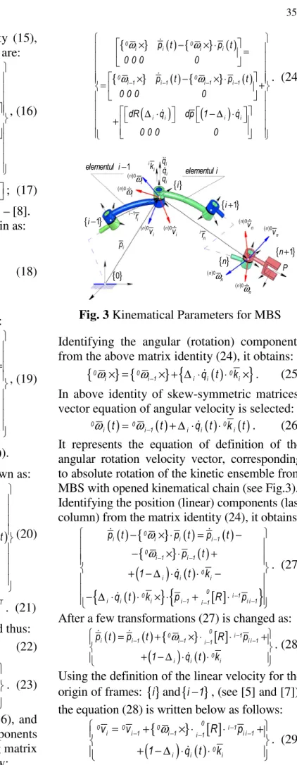
. (24)
Fig. 3 Kinematical Parameters for MBS
Identifying the angular (rotation) components from the above matrix identity (24), it obtains:
{
0} {
0}
{
( )
0}
i i 1 i q ti ki
ω × = ω− × + ∆ ⋅& ⋅ × . (25) In above identity of skew-symmetric matrices, vector equation of angular velocity is selected:
( )
( )
( )
( )
0 0 0
i t i 1 t i q ti k ti
ω = ω− + ∆ ⋅& ⋅ . (26)
It represents the equation of definition of the angular rotation velocity vector, corresponding to absolute rotation of the kinetic ensemble from MBS with opened kinematical chain (see Fig.3). Identifying the position (linear) components (last column) from the matrix identity (24), it obtains:
( ) {
} ( )
( )
{
}
( )
(
)
( )
( )
{
}
{
[ ]
}
0
i i i i 1
0
i 1 i 1 0
i i i
0
0 i 1
i i i i 1 i 1 i i 1
p t p t p t
p t
1 q t k
q t k p R p
ω ω
−
− −
−
− − −
− × ⋅ = −
− × ⋅ +
+ − ∆ ⋅ ⋅ −
− ∆ ⋅ ⋅ × ⋅ + ⋅
& &
&
&
. (27)
After a few transformations (27) is changed as:
( )
( ) {
}
[ ]
(
)
( )
0
0 i 1
i i 1 i 1 i 1 i i 1
0
i i i
p t p t R p
1 q t k
ω −
− − − −
= + × ⋅ ⋅ +
+ − ∆ ⋅ ⋅
& &
& . (28)
Using the definition of the linear velocity for the origin of frames:
{ }
i and{
i 1−}
, (see [5] and [7]), the equation (28) is written below as follows:{
}
[ ]
(
)
( )
0
0 0 0 i 1
i i 1 i 1 i 1 i i 1
0
i i i
v v R p
1 q t k
ω −
− − − −
= + × ⋅ ⋅ +
+ − ∆ ⋅ ⋅
&
. (29) { }0
{ }i−1
{ }i
{ }i+1
{ }n { }
1
n+ P
i
qqi
&i
q
&&
i i
k ( )n0
i
ω ( )n0
i
ω&
( )n0
n
ω ( )n0
n
ω& ( )n0
i
v ( )n0
i
v& ( )n0
n
v ( )n0
n
v&
i
p
1
i i
r −
i n
r
1
It represents the equation of definition of the linear velocity vector, corresponding to absolute
motion of the origin Oi∈
{ }
i belonging to kineticensemble from MBS with opened chain (Fig.3). Applying the absolute time derivatives of first order on (26) and (29), and performing a few differential transformations, the equations of definition for angular and linear accelerations
vectors are obtained:0
i
ω& and respectively0 i v& . But, especially in the dynamics equations the above kinematical parameters are required by
the components with respect own frame
{ }
i . Theangular and linear velocities and accelerations, corresponding to every kinetic ensemble (Fig.3) are below presented by means of the definition
equations with respect own frame
{ }
i thus:[ ]
ii i 1 i
i i 1 R i 1 i qi ki
ω −ω
− −
= ⋅ + ∆ ⋅& ⋅ ; (30)
[ ]
{
}
(
)
i
i i 1 i 1 i 1
i i 1 i 1 i 1 ii 1
i
i i i
v R v p
1 q k
ω ∆
− − −
− − −
−
= ⋅ + × +
+ − ⋅ ⋅
&
; (31)
[ ]
[ ]
{
}
i
i i 1
i i 1 i 1
i i 1 i i
i i 1 i 1 i i i i
R
R q k q k
ω ω
∆ ω
− − −
− − −
= ⋅ +
+ ⋅ ⋅ × ⋅ + ⋅
& &
& && ; (32)
[ ]
(
)
(
)
i
i i 1 i 1 i 1
i i 1 i 1 i 1 ii 1
i 1 i 1 i 1
i 1 i 1 ii 1
i i i
i i i i i i
v R v p
p
1 2 q k q k
ω
ω ω
∆ ω
− − −
− − −
−
− − −
− − −
= ⋅ + × +
+ × × +
+ − ⋅ ⋅ × ⋅ + ⋅
& & &
& &&
. (33)
They are function in exclusivity of parameters included in
[ ]
0 ; i kinematical interval [7]. So,they are applied by outward iterationsi=1→n.
When
(
i=1)
, within of the equations (30) – (33)the kinematical parameters of the fixe basis from MBS are substituted, according to next:
{
0 0 0 0}
0 0 , 0 0 , v0 0 , v0 0
ω = ω& = = & = . (34)
When
(
i=n)
, the kinematical parameters of thelast kinetic ensemble from MBS are obtained. They are operational velocities and accelerations:
( )
( )
( ) ( )
( )
( ) ( )
( )( ) ( )
{
}
n 0 6 1
T
n 0 T n 0 T
n n
X t ; t
v t ; t t ; t
θ θ
θ θ ω θ θ
×
=
& &
& &
; (35)
( )
( )
( ) ( ) ( )
( )
( ) ( ) ( )
( )
( ) ( ) ( )
n 0 6 1 n 0
n n 0
n
X t ; t ; t
v t ; t ; t
t ; t ; t
θ θ θ
θ θ θ
ω θ θ θ
×
=
=
&& & &&
& && &
& && &
; (36)
( )n 0
( ) ( )
( )n 0 ( )0 n( ) ( )
X&θ t ;θ& t = R⋅ X&θ t ;θ& t ; (37)
( )
( ) ( ) ( )
( ) ( )
( ) ( ) ( )
n 0 n 0 0 n
X t ; t ; t
R X t ; t ; t
θ θ θ
θ θ θ
=
= ⋅
&& & &&
&& & && ; (38)
( ) ( )
[ ]
( )[ ]
[ ]
[ ]
( )0 T
n 0 n
0 T
6 6
n
R 0
R
0 R
×
=
; (39)
The above expressions (35) and (37), as well (36) and (38) represent the linear and angular velocities as well accelerations, corresponding to motion of the last kinetic ensemble of MBS with respect to absolute Cartesian frame, [5] – [7]. To
these is added the locating matrix (3) for
(
i=n)
.The operational velocities and accelerations (35) and (36), according to [7] and [14], are also determined by means of the transfer matrices answerable to kinematical modeling of MBS. In the view of this, for beginning the orientation vector of the last kinetic ensemble of MBS is:
( )
t A( )
t B( )
t C( )
t Tψ =α β γ ; (40)
( )
( )
( )
(
)
(
) (
)
0
A B C
0
A A B
J t t t
A R A; B R A; R B; C
ψ α β γ
α α β
− − =
⋅ ⋅ ⋅
; (41)
( )
0( )
( )
( )
( )
A B C
t Jψ t t t t
ψ = α −β −γ ⋅ψ ; (42)
where (41) represents the angular transfer matrix defined as function of set of orientation angles. In the following, according to [7] – [14], column vectors corresponding to angular and linear transfer matrices for velocities and accelerations, as well as their time derivatives are presented for
(
i= →1 n)
. So, the equations of definition are:[ ]
[ ]
{ }
[ ]
( )
( )
0
0 i
i i i i i i
0 0 T
i
n n
i 0
i i
k R k
vect R R
q
J t t
q
ψ
Ω ∆ ∆
∆
ψ ∆
= ⋅ = ⋅ ⋅ =
∂
= ⋅ ⋅ =
∂
∂
= ⋅ ⋅
∂
; (43)
0
0 i 0 0
i ki i i R ki i i ki i
Ω& = & ⋅∆ = & ⋅ ⋅∆ = ω × ⋅∆ ; (44)
(
)
(
)
0 0
n
i i n i i i i
i p
V k p p 1 k
q ∆ ∆
∂
= = × − ⋅ + − ⋅
∂ ; (45)
(
)
(
)
2 n
n
i j
j 1 i j
0 0
i n i i i i
p
V q
q q
d
k p p 1 k
d t ∆ ∆
=
∂
= ⋅ =
∂ ⋅ ∂
= × − ⋅ + − ⋅
∑
& &
; (46)
The components (43) and (44), respectively (45) and (46) are corresponding to transfer matrices for angular and respectively linear velocities and accelerations. Finally, the following are obtained:
( )
( )
( )
( ) ( )
( ) 0
i 0
i
i
V t
J t ... t
V t
J t ... ; i 1 n t
θ θ
Ω θ
Ω
= =
= = = →
; (47)
( )
( )
( )
( )
( )
( )
0
i 0
i
i
V t
J t ...
t V t
J t ... ; i 1 n
t
θ θ
Ω θ
Ω
= =
= = = →
&
&
&
&
&
&
; (48)
( )n 0
( )
( )n 0 ( )0 n( )
Jθ t = R⋅ Jθ t ; (49)
( )n 0
( )
( )n 0 ( )0 n( )
J&θ t = R⋅ J&θ t . (50) According to [5] and [7], the matrix expression (47) represents the Jacobian matrix, also named the velocity transfer matrix, sometimes matrix of partial derivatives of the locating equations. The expression (48) is the time derivative of the Jacobian matrix, while (49) and (50) are the transfer relationships from one to another frame. The inverse of Jacobian matrix is determined as:
( )
1 0( )
T 0( )
1 0( )
T0Jθ Jθ Jθ ⋅ Jθ
⋅
=
− −
; (51)
( )
1 0( )
T 0( ) ( )
0 T 10J − J J J −
⋅
⋅
= θ θ θ
θ . (52)
When the mechanical robot structure (Fig. 1) is dominated by sudden motions, the generalized and operational accelerations of higher order are developed. Considering the researches from [7] – [14], in the paper the expressions become:
( )
( )
( )
( )( )
(
)
(
)
( )
( )
( )
[ ]
(
)
(
) (
)
( )
( )
( )
( )
m m
0 0
k m k
m 1
0 k 1
k 1 m k 1
m
0 k 1
X t J t t
m 1 !
J t t
k ! m k 1 ! m 1 !
J t t
k 1 ! m k !
θ θ
θ θ
θ θ
− −
=
− − −
=
= ⋅ +
−
+ ⋅ ⋅ =
− −
−
= ⋅ ⋅
− −
∑
∑
; (53)
where
( )
m is the order of the time derivatives,the symbol
( )
( )m
0X t represents the column matrix
of the operational accelerations of higher order,
and
( )
( )m
t
θ is the column matrix of generalized
accelerations of higher order, according with:
( )
( )
( )
( )
( )
( )
(
)
(
)
( )
( )
( )
( )
m m
1
0 0
k m k
m 1 1
0 0
k 1
t J t X t
m 1 !
J t J t t
k ! m k 1 !
θ θ
θ θ θ
−
− −
−
=
= ⋅ −
−
− ⋅ ⋅ ⋅
− −
∑
(54)
Considering the mathematical models from [7], the Jacobian matrix (47) can be also determined with matrix exponentials. But, the components of (53) and (54) are based on rotation matrices and position vectors, according (43) – (48). So, their time derivatives of higher order show as:
( )
( ) ( )
( )
( ) ( )
k k
0 0
i i
6 n 6 1
J θ t J θ t where i 1 n
× ×
≡ = →
; (55)
( )
( ) ( )
( )
( )
( )
( )
k
k i
0 i i
k 6 1
i V t
J t
t
θ
×
=
Ω
... ; (56)
[ ]
( ){
}
[ ]
( )
( )
{ }
[ ]
( )( )
( )
( )
{ }
[ ]
( )( )
( )
{ }
[ ]
( ) ( )( )
( ) ( )
[ ]
( )
k m
k i k
0 0 0
j j
k i i m S
j 1 j r
m
p k p
i k 1
0 p 1
j j
p m S
j 1 r 1
j
m k
i
0
j j m S
j 1 j r
m p 0 p 1
m S j d
R t R R q
d t q
k p d
R q
p! dt q
R q
q
k p
p ! m !
R
p! m p ! q
=
− −
= = =
=
+ =
∂
= = ⋅ ∆ ⋅ +
∂
−
∂
⋅ ⋅ ∆ ⋅ =
∂
∂
= ⋅ ∆ ⋅ +
∂
−
⋅ ∂
⋅ ⋅
+ ∂
∑
∏
∑∑
∑
∏
(k p)i k 1
j j j 1 r 1
q − −
= =
⋅ ∆ ⋅
∑∑
( )
( ) ( )( )
( )
(
)
(
)
( )
( )
( )
m
k k i k
i i
i j
k m
j 1 j r
m p k p i k 1
p 1 i
j m j 1 r 1
j
d p t p
p q
d t
q
k p
p p! m !
q p! m p ! q
=
+ − −
=
= =
∂
= = ⋅ +
∂
−
∂ ⋅
⋅ ⋅ ⋅
+
∂
∑
∏
∑∑
(57)
and
{
}
(
)
{
}
k 1; k 1; 2; 3; 4;5; ...
m k 1 ; m 2; 3; 4;5; ...
≥ =
≥ + =
; (58)
where the symbols:
( )
k and( )
m are the orders3. GENERALIZED ACTIVE FORCES
In accordance with [3], [4] and [7], on every
kinetic ensemble
(
i= →1 n)
, belonging to themechanical robot structure, as integrated part from MBS, are especially applied a system of external and active forces, manipulating loads,
as well as complex friction forces, see Fig.4.
Fig. 4 Distribution of the forces on MBS In function of (static or dynamic) behavior in every physical link (driving joint of fifth order) generalized static or driving force is developed.
For beginning, using the classical algorithm
[4] and [7], generalized forces corresponding to static equilibrium are established. Considering theorems from statics of mechanical systems and a few transformations, the next expressions are
obtained by inward iterations
(
i= →n 1)
, thus:[ ]
[ ]
0 T i
i i 1
i i i i 1 i 1
f M R g R + f+
+
= ⋅ ⋅ + ⋅ ; (59)
[ ]
[ ]
[ ]
i
0 T
i i
i C i i
i i
i i 1 i 1
i 1 i 1 i 1 i 1 i 1
n r R g M
r+ + R +f+ + R +n+
= × ⋅ ⋅ +
+ × ⋅ + ⋅
; (60)
{
} { }
0 0 0 0 0
g= ⋅ ⋅τ g k , and k = x ; y ; z ∈ 0 frame; (61)
T g 0
T 0 0
g 0 T g
g 0
1; k k 1
k k , k g g
1; k k 1
τ = − ⋅ =− ⋅ = =
⋅ = −
; (62)
(
)
i i T i T i
S i i i i i
Q = f ⋅ − ∆ +1 n ⋅ ∆ ⋅ k . (63) The symbols from above expressions have the following significances: ifi andini are the action
(force and moment of force) from
(
i 1−)
on( )
iensemble of MBS (Fig.4); Mi and
i
i C
r are mass
and position of the mass center; g module of
gravitational acceleration (61); i
S
Q is generalized
static force (63). It observes that all vectors are
projected on driving axis whose unit vector isiki.
To highlight the influence of gravitational and manipulating loads, (59) and (60) are written as:
[ ]
( )
M[ ]
n
0 T
i 2
i m j i
j i
i n 1
m
n 1 n 1
m
f M R g
1
1 R f
1
∆
∆ ∆ ∆
=
+ + +
= ⋅ ⋅ ⋅ +
−
+ − ⋅ ⋅ ⋅
+
∑
; (64)
[ ]
(
)
( )
{
[ ]
(
)
[ ]
[ ]
}
j
m
n
0 T
i 2 0
i m j i C i
j i
0 T i
m n 1
i n 1
i n 1
m
i n 1
n 1 n 1
n M R r p g
1
1 R p p R f
1
R n
∆
∆
∆ ∆
=
+ + +
+ + +
= ⋅ ⋅ ⋅ − × +
−
− ⋅ ⋅ ⋅ − × ⋅
+
+ ⋅
∑
(65)
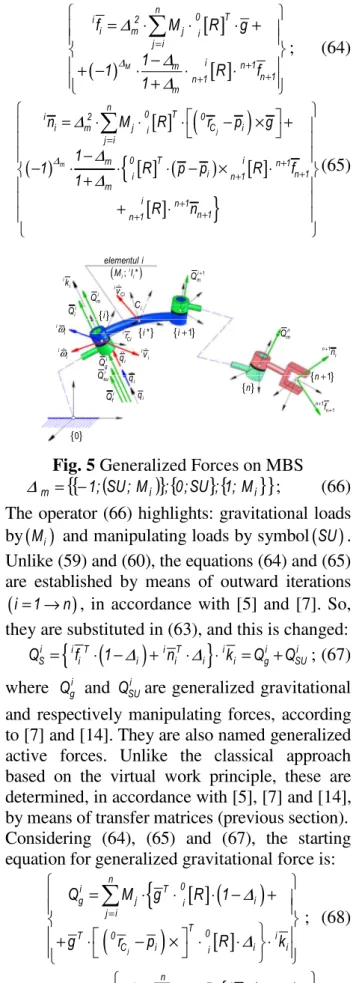
Fig. 5 Generalized Forces on MBS
(
)
{
} {
} {
}
{
i i}
m = −1; SU;M ; 0;SU ;1;M
∆ ; (66)
The operator (66) highlights: gravitational loads
by
( )
Mi and manipulating loads by symbol(
SU)
.Unlike (59) and (60), the equations (64) and (65) are established by means of outward iterations
(
i= →1 n)
, in accordance with [5] and [7]. So,they are substituted in (63), and this is changed:
(
)
{
}
i i T i T i i i
S i i i i i g SU
Q = f ⋅ 1−∆ + n ⋅∆ ⋅ k =Q +Q ; (67)
where i
g
Q and i
SU
Q are generalized gravitational
and respectively manipulating forces, according to [7] and [14]. They are also named generalized active forces. Unlike the classical approach based on the virtual work principle, these are determined, in accordance with [5], [7] and [14], by means of transfer matrices (previous section). Considering (64), (65) and (67), the starting equation for generalized gravitational force is:
[ ]
(
)
{
(
j)
[ ]
n
0
i T
g j i i
j i
T 0
T 0 i
C i i i i
Q M g R 1
g r p R k
∆ ∆
=
= ⋅ ⋅ ⋅ − +
+ ⋅ − × ⋅ ⋅ ⋅
∑
; (68)
[ ]
0 i 0
i i
i R ⋅ k = k ;
(
)
{
(
j)
}
n
i T 0
g j i i
j i
0 0
i C i i
Q M g k 1
k r p
∆ ∆
=
= ⋅ ⋅ ⋅ − +
+ × − ⋅
∑
(69)
{ }0
i f
Q
i su
Q
i g
Q
i
q
& i
q
&& i
q iv&i
{ }i
ω& i
i ω i
i i i
Q
i m
Q
i i
k
i Ci
r
& i
Ci
v
i
C elementul i ( ;i*)
i i
M I
{ }i* {i+1}
+1
i m
Q
n m
Q
{ }n
{n+1}
+1
n n
n
+ +
1 1
n n
f
{ }0
i p
{ }i i
i n
+ +
1 1
i i n
+ +
1 1
n n n i
i N i
i f
+ +
1 1
i i f
+ +
1 1
n n f i
i F i
Ci r
i
C { }i* +1
i i r
elementul i
( ;i*) i i M I
0
Cj r
j Cj r
0
j G j C
n p
nj p elementul j
{ }n
{n+1} {i+1}
+1