Diversity-Multiplexing Trade-off for Coordinated
Direct and Relay Schemes
Chan Dai Truyen Thai, Petar Popovski,
Senior Member, IEEE,
Elisabeth de Carvalho,
Member, IEEE,
and Fan Sun
Abstract—The recent years have brought a significant body of research on wireless Two-Way Relaying (TWR), where the use of network coding brings an evident advantage in terms of data rates. Yet, TWR scenarios represent only a special case and it is of interest to devise similar techniques in more general multi-flow scenarios. Such techniques can leverage on the two principles used in Wireless Network Coding to design throughput-efficient schemes: (1) aggregation of communication flows and (2) embracing and subsequently cancel/mitigate the interference. Using these principles, we investigate Coordinated Direct/Relay (CDR) schemes, which involve two flows, of a direct and a relayed user. In this paper we characterize a CDR scheme by deriving/bounding the Diversity-Multiplexing Trade-off (DMT) function. Two cases are considered. In the first case a transmitter knows the Channel State Information (CSI) of all the links in the network, while in the second case each node knows only CSI of the links towards its neighbors. The results show that the new CDR scheme outperforms the reference scheme in terms of DMT characterization. Several interesting features are identified with respect to the impact of the CSI knowledge to the improvement in diversity or multiplexing brought by the CDR scheme.
I. INTRODUCTION
A. Motivation
Relay–based transmission, has been a subject of extensive research efforts in the recent years, due to its potential to extend cellular coverage or increase diversity. Several relaying modes have been established, such as Amplify-and-Forward (AF) [1], Decode-and-Forward (DF) [2] and Compress-and-Forward (CF) [3], etc. These modes have been used as building blocks to devise relaying techniques in relaying scenarios with one, two, or multiple communication flows [4].
In particular, Two-Way Relay (TWR) using Wireless Net-work Coding (WNC) has recently attracted a significant
Manuscript received May 20, 2012; revised Oct 12, 2012 and Feb 26, 2013.
This work is supported by the Danish Research Council for Technology and Production, grant nr. 09−065035 and 09−065920 and by the CISIT (International Campus on Safety and Intermodality in Transportation) program of the North Region, the French State and the European Commission (FEDER).
Part of this work has been performed in the framework of the FP7 project ICT-317669 METIS, which is partly funded by the European Union. The authors would like to acknowledge the contributions of their colleagues in METIS, although the views expressed are those of the authors and do not necessarily represent the project.
Chan Dai Truyen Thai was with Department of Electronic Systems, Aalborg University, Denmark. He is now with IFSTTAR, LEOST, Villeneuve d’Ascq, France (email: [email protected]).
Petar Popovski, Elisabeth de Carvalho and Fan Sun are with De-partment of Electronic Systems, Aalborg University, Denmark (email:
{petarp, edc}@es.aau.dk, [email protected]).
interest, due to the evident throughput benefits in wireless networks [5]–[7]. Schemes applying WNC in TWR scenarios have been extensively discussed, analyzed and evaluated in many different aspects. Yet, the TWR scenarios are essen-tially limited, as they represent a special case of the general scenario in which multiple communication flows need to be concurrently transmitted over a shared wireless medium. In order to generalize the transmission schemes applied in TWR scenarios, it is instructive to identify the two basic principles used in designing throughput–efficient schemes with WNC: (1)
aggregation of communication flows: WNC operates by having a set of flows sent/processed jointly; (2)intentional cancelable interference using side information: flows are allowed to interfere over the wireless channel, knowing a priori that the interference can be cancelled by the destination via side information.
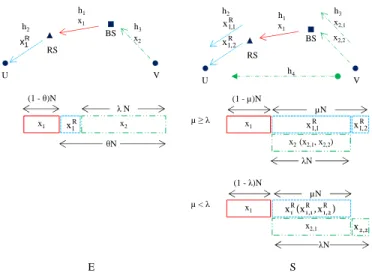
Using these principles one can design novel transmission schemes in other multi-flow scenarios that involve wireless relaying. A particularly promising scenario is a network with a base station (BS), a relay station (RS), a relayed user (U) and a direct user (V). One possible configuration of multiple traffic flows is depicted on Fig. 1, where user U receives downlink traffic from the BS, while V sends uplink traffic to the BS. In the first step the BS transmits to the relay RS. For the reference schemeE, in the second step RS transmits to user U and in the third step V transmits to the BS. However, using the principles behind WNC, we can do better in the following way. By recognizing that the BS knowsa prioriwhat RS will send in the second step because the relayed signal from RS is what was originally transmitted by the BS, the new schemeS operates by combining both transmissions RS→U and V→BS in the same step. Then BS can cancel the signal sent by the RS and obtain a “clean” message from V. This scheme has been proposed in [10]. The same scenario can be used as a basis to design transmission schemes for other configurations of traffic flows. One example is when U has an uplink traffic towards BS through the RS, while V has a downlink traffic from the BS. The latter and two more schemes have been discussed and analyzed in [11]. Detailed analysis of the achievable rate regions in these traffic scenarios is provided in [4] (AF) and [12] (DF).
transmission phase durations of TWR Network Coding. We focus on the scenario and the traffic configuration depicted on Fig. 1 (from now on referred to simply as “the scenario”) and we derive the DMT functions for both the reference scheme and the scheme S from [10]. We are using DF as a relaying method, which means that the relay is able to re–encode the information that is relayed with another codebook. The transmissions rates from the BS to the RS and from the RS to user U are not necessarily identical, leading to time intervals that are not necessarily equal. The essential difference with [14] is that in the two-phase two-way relaying scheme in [14], the interference is a priori known and completely cancelled while in this paper part of the interference is cancelled and part is treated as noise. We thus introduceβ as a power exponent to distinguish the transmit powers of different sources. As a technical difference, we need to optimize over multiple variables that represent the time intervals, rather than one variable as in [14].
The DMT function of S depends on three different trans-missions, two of which (RS→U and V→BS) are taking part simultaneously. In fact, due to the use of DF, the transmissions of RS and V in the second step of the scheme S are not necessarily completely overlapping. The durations/overlaps of all transmissions are therefore different and subject to opti-mization, through which one minimizes the outage probability.
B. Main Contributions
The main contributions of this paper can be described as follows. We consider two possible configurations of channel knowledge in the network. In the first case, termed CSI-L
(Channel State Information for the related Link channels), each node knows only the CSI of the links towards its neighbors. In the second model, termed CSI-A(Channel State Information for All channels), the information of all channels is available at all stations. The transmission strategies and the DMT functions are significantly different for the two cases. We analytically calculate the DMT function of the reference scheme, denoted byE, and the CDR scheme in CSI-L model. In CSI-A model the DMT functions are bounded.
• In the case of CSI-L, due to the fact that not all channels in the network are known, the durations of the different transmissions cannot be optimized for the instantaneous fading realizations, i.e. the actual channels that are valid during the time block in which the transmission takes place. Instead, for given rates, these durations are fixed and optimized according to the statistics of the individual links.
• In the case of CSI-A, for each fading realization one can optimize the durations of the different steps. Outage occurs if, for the fading realizations in the observed time block, there are no time durations that can satisfy the required rates.
The rest of the paper is organized as follows. Section II presents the system model used. We describe and calculate the maximal achievable rates of the reference and CDR schemes in Section III. Section IV calculates and bounds the DMT functions of the schemes. Section V presents and discusses the numerical results and Section VI concludes the paper.
BS RS
x2,2
x1
V U
µN µ ≥ λ
x2 (x2,1, x2,2)
λN x1 x2,1
R 2 , 1
x
R 1 , 1
x R
2 , 1
x
R 1 , 1
x
x1
(1 -θ)N
λ N x2
R 1
x
h1
h3
h2
h4
θN
(1 - µ)N BS
RS
V U
x1
x2 R
1 x
h1
h3
h2
λN
E
x1
µN
x2,1
λN
) x , x (
x R
2 , 1 R
1 , 1 R 1
2 , 2
x
(1 -λ)N µ < λ
S
Fig. 1. Reference E and S CDR Schemes. In each scheme, the time interval of the transmission represented by an arrow above is represented by a rectangular below with the same color and the transmissions represented by the rectangles in the same column are conducted simultaneously.
II. SYSTEMMODEL
We consider a scenario with one base station (BS), one relay (RS), and two users (U and V), see Fig. 1. All stations have a single antenna and all transmissions have a normalized bandwidth of 1 Hz. Each of the complex channels hi, i ∈
{1,2,3,4}, is reciprocal and a realization of a block fading Rayleigh distribution. The variance of each channel is set to 1. We consider two channel models. In the first one, only the transmitter and the receiver of a transmission know the channel of that transmission (CSI-L). In the second one, information of all channels is available at all stations (CSI-A). The direct channel BS–U is assumed weak and U gets the information from BS only through the decoded/forwarded signal from RS. BS has to send message s1 to user U via relay RS and
receive messages2 from user V directly. Because we have a
relayed downlink and a direct uplink, there are three relevant links: BS→RS, RS→U, V→BS, corresponding to the channels h1, h2 and h3, respectively. We assume that the transmit
powers of the corresponding transmitters are PB, PR, PV,
respectively. In addition, we assume PB = PR = ρ and
PV =ρβ[16]. The noise at all stations has a complex circular
Gaussian distribution with varianceσ2
N set to 1. We denote the
number of symbols in codewordxas|x|,logdenotes the base-2 logarithm and,serves to define a notation via an equation. In the reference scheme denoted as E, all transmissions are orthogonally multiplexed in time. In the CDR scheme denoted asS, transmissions of the two messages are partially overlapped in time. This overlap time is chosen in such a way that the information about the interference is exploited as much as possible. We use RiU and RiV, i ∈ {E, S} to denote the maximal achievable rates averaged over the whole duration of schemeifor users U and V respectively.
symbols in the whole scheme. In schemeE, there are totally θN symbols in the RS→U and V→BS hop transmissions. In scheme S, there are µN symbols in the RS→U hop transmission.
Finally, we use yk[j] andzk[j] to denote the received and
noise signals respectively at stationk,k∈ {B, R, U, V}where B, R, U and V are corresponding subscripts for BS, RS, users U and V, in time intervalj,j∈ {1,2,3} andqi
U[j]andqVi [j]
as instantaneous transmission rates in time intervaljfor user U and V respectively in schemei,i∈ {E, S}. Denoteγi= |
hi|2 σ2
N
withi∈ {1,2,3,4}. The notation summary is given in Table I.
III. SCHEMEDESCRIPTION
We describe and calculate the achievable rates for two users in the reference scheme E and the CDR schemeS.
A. Reference Scheme
The reference scheme consists of three transmission phases. In the first transmission phase, BS encodes s1 tox1 at a rate qUE[1] and transmits it to RS as seen in Fig. 1. RS receives
yR[1] =h1x1+zR[1]. In the second transmission phase, RS
decodes x1 to s1, re-encodes it to xR1 at a rate qEU[2] and
transmits it to user U. U receives yU[2] =h2xR1 +zU[2]. In
the third transmission phase, user V encodess2tox2at a rate qE
V[3] and transmits it to BS. BS receives yB[3] = h3x2+ zB[3]. Since x1, x2 and x3 are transmitted with power PB,
PR and PV, the rates qUE[1],qEU[2]andqEV[3]are selected as
the maximal rates over the corresponding channels qE
U[1] =
log (1 +ργ1),C1,qEU[2] = log (1 +ργ2),C2andqEV[3] =
log 1 +ρβγ
3,C3.
Since all transmissions are performed separately, the dura-tion of the BS→RS transmission is (1−θ)N. The BS→RS, RS→U and V→BS transmissions therefore have durations of
(1−θ)N, (θ−λ)N and λN symbols respectively. On the other hand, the corresponding maximal rates are C1,C2 and C3for each of the respective transmissions. Thus the maximal
rates for the transmissions on the links BS→RS, RS→U and V→BS are
RE U1=
(1−θ)N C1
N = (1−θ)C1, R E
U2 = (θ−λ)C2,
RE
V =λC3.
(1)
B. CDR Scheme
The RS→U and V→BS transmissions can be conducted simultaneously because the interfering signal from RS to BS is known at BS and can be cancelled. Therefore compared to the reference scheme, the maximal rates will be increased.
In the first time interval, BS transmits x1 to RS (see
Fig. 1), RS receives yR[1] = h1x1 +zR[1] and decodes
x1 to s1. The maximal achievable rate of this transmission
is therefore qUS[1] = C1. In the second time interval, two
cases are distinguished depending on the relative duration of transmissions RS→U and V→BS.
1) µ≥λ: In the second time interval, user V encodess2to x2and RS dividess1 into two sub-messagess1,1 ands1,2 so
that after re-encoding toxR
1,1andxR1,2, we have|xR1,1|=λN.
RS transmits xR
1,1 to user U and user V transmits x2 to BS
simultaneously. BS thus receives yB[2] = h1x1R,1+h3x2+ zB[2]. Since BS knows x1, it can cancel the contribution of x1and decodes its desired signalx2with maximal achievable
rate C3. In the meantime, user U receives yU[2] =h2xR1,1+ h4x2+zU[2]. There are two decoding options for user U:
• No-Interference Cancellation (NIC): User U decodesxR1,1 treating x2 as noise. The maximal achievable rate for
transmitting xR1,1 isqUS[2] = log
1 + ργ2
ρβγ
4+1
,C2−4.
The transmitting rate ofx2 is selected asqSV[2] =C3.
• Interference Cancellation (IC): User U first decodes x2
treating xR1,1 as noise. It is possible only if the
trans-mitting rate of x2 is not larger than log
1 + ρβγ4
ργ2+1
,
C4−2. Hence the transmitting rate of x2 is selected as
qSV[2] = min{C3, C4−2}. Then user U cancels x2’s
contribution inyU[2]and decodesx1,1 interference-free.
Hence the maximal achievable rate for transmitting x1,1
isqS
U[2] =C2.
A trade-off between those two options can be achieved by mul-tiplexing them by time. It is actually one point in the diagonal edge of the Multiple Access Channel (MAC) rate region when user U treats the interference from user V as another signal to decode [15]. In terms of sum-rate, this trade-off solution can be better than both NIC and IC decoding options above. However, when computing the DMT, the transmit powers tend to infinity. Depending on which of RS and user V’s powers goes to infinity faster, the only relevant decoding options are either NIC or IC.
In the third time interval, RS transmits xR1,2 to user U interference-free with rateqS
U[3] =C2.
The durations for the three time slots are therefore(1−µ)N, λN and(µ−λ)N symbols respectively. The maximal achiev-able rates averaged over the whole duration of the scheme are,
• For links BS→RS, RS→U and V→BS in the NIC option, RSU
1 = (1−µ)C1, R
S
U2 = λC2−4 + (µ−λ)C2 and
RS
V =λC3.
• For links BS→RS, RS→U, V→U and V→BS in the IC option, RS
U1 = (1−µ)C1, R
S
U2 = µC2 and R
S V =
λmin(C3, C4−2) + (µ−λ) min(C3, C4).
Selecting a decoding option will be discussed later on.
2) µ < λ: In the second time interval, RS encodes s1 to xR
1 and user V dividess2into two sub-messagess2,1ands2,2
so that after re-encoding to x2,1 and x2,2, we have |x2,1| = µN. RS transmits xR1 to user U and user V transmits x2,1
to BS simultaneously. The NIC and IC options are conducted similarly as in the caseµ≥λ. In the third time interval, user V transmitx2,2 to BS.
The durations for the three time slots are (1−λ)N, µN and(λ−µ)N symbols respectively. The maximal achievable rates averaged over the whole duration of the scheme are,
• For links BS→RS, RS→U and V→BS in the NIC option, RS
U1 = (1−λ)C1,R
S
U2 =µC2−4 andR
S
TABLE I
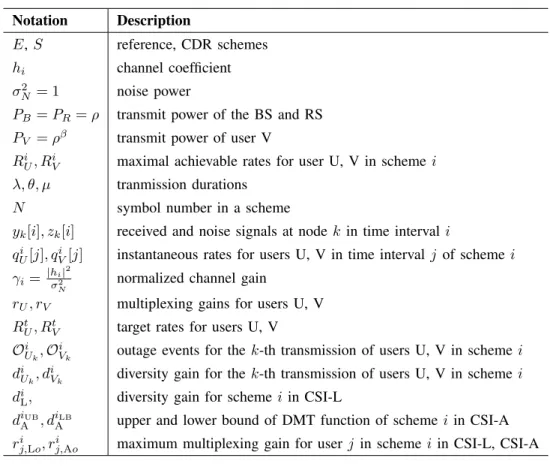
NOTATIONSUMMARY
Notation Description
E,S reference, CDR schemes
hi channel coefficient
σ2
N = 1 noise power
PB=PR=ρ transmit power of the BS and RS
PV =ρβ transmit power of user V
Ri
U, RiV maximal achievable rates for user U, V in schemei
λ, θ, µ tranmission durations
N symbol number in a scheme
yk[i], zk[i] received and noise signals at nodekin time interval i
qi U[j], q
i
V[j] instantaneous rates for users U, V in time interval j of scheme i
γi= |hi|
2
σ2
N
normalized channel gain
rU, rV multiplexing gains for users U, V
RtU, RtV target rates for users U, V
Oi Uk,O
i
Vk outage events for thek-th transmission of users U, V in schemei
di Uk, d
i
Vk diversity gain for thek-th transmission of users U, V in schemei
diL, diversity gain for scheme iin CSI-L
diUB
A , d
iLB
A upper and lower bound of DMT function of schemei in CSI-A ri
j,Lo, r i
j,Ao maximum multiplexing gain for userj in schemei in CSI-L, CSI-A
• For links BS→RS, RS→U, V→U and V→BS in the IC option, RS
U1 = (1 − λ)C1, R
S
U2 = µC2 and
RS
V = µmin{C3, C4−2}+ (λ−µ) min(C3, C4) with
C4,log 1 +ρβγ4
.
IV. DIVERSITY-MULTIPLEXINGTRADE-OFF(DMT) ANALYSIS
We first introduce the DMT definition and notations in section IV-A and derive the DMT functions in both channel modes CSI-L and CSI-A forEin section IV-B andSin section IV-C.
A. DMT Definition and Notations
A scheme is said to achieve spatial multiplexing gainrand diversity gaindif
limζ→∞Rlog(ζζ)=r and limζ→∞−loglogPeζ(ζ)=d (2)
where R(ζ) is the maximal achievable rate, ζ is the corre-sponding average SNR andPeis the average outage
probabil-ity.
Throughout the rest of the paper, we use the symbol =.
to denote exponential equality, i.e. we write f(ζ) =. ζb
then limζ→∞loglogf(ζζ) = b. Notations and .
≥, ≤. are similarly defined. Therefore, the second equation in (2) can be written as
Pe(ζ)
.
=ζ−d. (3)
We also denote (x)+ = max(0, x). Because
limζ→∞ ζ
a+ζb
ζmax(a,b) = 1, we often use ζ
a +ζb =. ζmax(a,b) or
ζa+ 1 =ζa+ζ0=. ζmax(a,0)=ζa+. Moreover,
Pr[γi < x] =
Z x
0
e−tdt= 1−e−x and lim
x→0
1−e−x
x = 1.
(4) Therefore,
Pr
γi < ζ−a=. ζ−a
+
. (5)
We investigate the outage probability and how fast it decays with respect to logPi,i∈ {B, R, V}, when the system tries
to achieve a certain target rate pair(RtU, RtV).
Since the stations have different transmit powers, the target rates have different expressions. We calculate the DMT for the scheme when the target rate for user i is given byRt
i =
rilogPj whereri is the corresponding multiplexing gain and
Pjis the transmit power of the transmitter i.e. for direct uplink
Pj =PV =ρβ and for relayed downlinkPj =PB =ρ. We
assume that β is always known in both cases of CSI-L and CSI-A.
factors. For example, in scheme S, if the transmission from the BS is allocated a short duration compared to the 2 other simultaneous transmissions, the rate to user U computed over the whole duration of the scheme will likely be small and below the target rate.
In the CSI-L model of scheme E, an outage is defined if the pair (λ, θ) cannot support a target rate pair(Rt
U, RtV). The
outage probability and then the DMT function are calculated as functions of λandθ. The DMT function is maximized based on λ and θ. In the CSI-A model of scheme E, all channels are available thus for a certain channel realization, λ and θ are calculated so that they can support a target rate pair for the given fading realization. An outage is defined as there is not any pair(λ, θ)which can support the target rate pair [14], [17], [18]. A similar procedure is carried out in both channel models of scheme S with parameters(λ, µ).
B. Reference Scheme E
1) CSI-L:
Proposition 4.1: The DMT function of schemeE in CSI-L channel model is given bydE
L = min
dE U1, d
E U2, d
E
V in which
dE U1 =
1− rU
1−θ
+
, dE U2=
1− rU
θ−λ
+
,
dEV =β 1−rV λ
+ (6)
are the DMT functions of three transmissions BS→RS, RS→U and V→BS in the scheme respectively.
Proof: The scheme is in outage, denoted as OE, when
either Rt
U is larger than the maximal achievable rateR E U for
user U orRt
V is larger than the maximal achievable rateR E V
for user V. Recalling thatRE
U = min(R
E U1, R
E
U2), the system is in outage when one of the following conditions occur
OE U1 :R
E U1< R
t U, O
E U2:R
E U2 < R
t U, O
E V :R
E V < R
t V.
(7) Hence OE
L =O
E U1∪ O
E U2∪ O
E
V, where subscript L refers to
CSI-L. The probability of the first event is
PrOE
U1
= Pr[(1 +ργ1)1−θ< ρrU]
.
= Pr[(ργ1)1−θ< ρrU]
= Pr[γ1< ρ
rU
1−θ−1].
(8) The second equality in (8) is obtained when lettingρtend to infinity. This probability decays only when rU
1−θ −1 < 0. It
means that we have a positive diversity gain corresponding to this transmission only when 1− rU
1−θ >0. Using (5), we
can writePr OE
U1 .
=ρ−(1−1rU−θ)
+
. Similarly, the probability
of the second event is Pr OE
U2 .
= ρ−(1−θ−λrU )
+
. We have
Pr
OE V
.
=ρ−β(1−rVλ )
+
. Therefore,
Pr[OE
L] .
= Pr[OE
U1] + Pr[O
E
U2] + Pr[O
E V]
.
=ρmax{−dEU1,−dEU2,−dEV}=ρ−min{dEU1,dEU2,dEV}. (9)
The first equality comes from the fact that the eventsOE U1,O
E U2 andOE
V are independent due to the independence ofγ1,γ2and γ3and that the product of any two or three of the probabilities
Pr[OE
U1], Pr[O
E
U2] and Pr[O
E
V] decays faster than each of
them. The second equality is due to that the smaller terms are negligible and the probability is determined by the largest
term in the sum whenρ→ ∞. According to the definition in (3), the diversity gain is thereforedE
L = min dEU1, d
E U2, d
E V
,
fE
L(θ, λ, rU, rV).
The information in CSI-L channel model is necessary and enough to achieve the result above. At a station, the information of all channels is not available thus determining the transmission durations according to the current channel realization is impossible. Therefore, as shown above, the results in (6) is obtained by averaging all channel realizations. The optimal transmission durations will be then optimized based on these averaged results. On the other hand, the information of the channels to the neighbors of a station is still necessary such that it can determine the instantaneous rates to transmit and receive e.g. in the second time interval of schemeE, the RS needs to knowh2to determineqUE[2] =C2.
However this information does not help to determine the optimal transmission durations as all channels are assumed to be independent.
Proposition 4.2: The DMT function of schemeEin CSI-L channel model with optimized transmission durations is given by
dELo=
1− rU
1−θo
+
=
1− rU
θo−λo
+
=β
1−rV
λo
+ .
(10) in which θo= λo2+1,λo= 1−β−βrV−2rU+
√
∆
2(1−β) and∆ = (1−
β−βrV −2rU)2+ 4(1−β)βrV.
Proof: Each individual diversity component dE
U1, d
E U2, d
E V
increases when the corresponding time assigned to each transmission, (1 − θ)N, (θ − λ)N and λN respectively, increases. The time durations assigned to the 3 transmission hops should be balanced such that the diversity gain of the whole scheme is maximized. Note that increasing the diversity gain at a certain multiplexing gain also makes the multiplexing gain at a certain other diversity gain increased. Therefore maximizing diversity gain is equivalent to maximizing the multiplexing gain. Hence, with finite β, the optimal values λo and θo are roots of the equations dEU1 = d
E U2 = d
E V.
The equations dE
U1 = d
E
U2 = d
E
V are equivalent to
(1−β)λ2−(1−β−βrV −2rU)λ−βrV = 0andθ= 1+2λ.
Because ∆ = (1−β −βrV −2rU)2+ 4(1−β)βrV ≥ 0,
there are always real roots. We consider two cases
• β≤1, the two roots satisfiesλ1λ2=−β(1−β)rV ≤0,
there is hence one positive root.
• β > 1, λ1λ2 = −β(1−β)rV > 0 and λ1 +λ2 = 1−β−βrV−2rU
1−β >0, there are hence two positive roots.
We select the root as written in Proposition (4.2) which satisfies 0< λ < θ <1.
2) CSI-A: For the CSI-A case we have only derived the upper bound, similar to the approach in [13], [14].
Proposition 4.3: The upper bound of the DMT function of schemeE in CSI-A channel model is given by
dEUB
A =
β(1−2r
U−rV) 1−2rU
+
if β≤1
1−2rU−rV 1−rU−rV
+
if β >1.
θ
a2 1– a1
µ = λ+ a2
a3 λ
O
Fig. 2. Only in the shaded triangle in the middle, the scheme is not in an outage (λ≥a3,θ≤1−a1andθ≥λ+a2).
Proof:When all channels are available at all stations, the value ofλandθcan be selected according to all CSIs. User U and BS can decode the messagess1ands2respectively when
RE U1 ≥R
t U, R
E U2 ≥R
t U, R
E V ≥R
t
V. (12)
Denoting a1 , log(1+rUlogργρ
1), a2 ,
rUlogρ
log(1+ργ2) and a3 ,
rVlogρβ log(1+ρβγ
3), equation (12) is equivalent to
θ≤1−a1, λ≥a3 and θ≥λ+a2. (13)
We illustrate condition (13) in Fig. 2 with a coordinate system of λandθ in which the shaded area represents the values of λandθ which satisfy the conditions in (13). This non-outage area does not exist if and only if the point (a3,1−a1) lies
below the line θ = λ+a2. This condition is equivalent to
1−a1< a3+a2 or
a1+a2+a3>1. (14)
Equation (14) is the condition for an outage event, denoted as OE
A, for the CSI-A model. Denote αi = −loglogγρi, i ∈
{1,2,3,4} therefore a1 .
= rUlogρ
log(ργ1) =
rU 1−α1,a2
.
= rUlogρ
log(ργ2) =
rU
1−α2 anda3
.
= rVlogρβ
log(ρβγ
3)
.
= rV
1−α3
β
hence
Pr[OE
A] = Pr
h
rU 1−α1 +
rU 1−α2 +
rV 1−α3
β
>1i. (15)
Whenρ→ ∞,αi→0,α1α2,α2α3,α3α1andα1α2α3decay
faster than α1,α2 or α3 hence
Pr[OE
A] .
= Pr [rU(β−βα2−α3) +rU(β−α1−α3)
+rV(β−βα1−βα2)> β−βα1−βα2−α3].
(16) Because the time is divided for two transmissions of user U and one tranmission of user V we have rU +rV < 1 and
2rU <1. Using these conditions, we have two cases below
respectively. We therefore obtain lower bounds on the outage probability and thus upper bounds on the DMT functions for both cases as in (17). The upper bound of the DMT function is therefore given by (11).
It is obvious that Pr[OE
A] monotonically decreases with ρ whenever β(11−−23rr) is positive. Therefore −logρPr[OE
A]
monotonically increases with ρ. A lower bound of the DMT function can be hence obtained by calculating Pr[OE
A] at a
fixed value ofρ=ρo. The higherρo is, the tighter the lower
bound is. From (15), the condition rU 1−α1+
rU 1−α2+
rV 1−α3
β
>1is
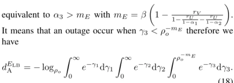
equivalent toα3> mE withmE =β
1− rV
1−1−αrU 1−
rU
1−α2
.
It means that an outage occur whenγ3< ρ−omE therefore we
have
dELB
A =−logρo
Z ∞
0
e−γ1dγ
1
Z ∞
0
e−γ2dγ
2
Z ρ−omE
0
e−γ3dγ
3.
(18) This bound is numerically calculated and given in section V.
C. Coordinated Direct and Relay SchemeS
In the CDR scheme S, there are two decoding options at user U. Whenβ≤1, the NIC option treating the interference from user V (with transmit powerρβ) as noise is better than the
IC option decoding the interference first. On the other hand, in the NIC option, the three transmission hops BS→RS, RS→U and V→BS have corresponding normalized ratesRS
U1= (1−
max(µ, λ))C1, RSU2 = min(µ, λ)C2−4+ (µ−min(µ, λ))C2
andRS
V =λC3. We have
• Ifµ≥λ,RS
U1 = (1−µ)C1,R
S
U2 =λC2−4+ (µ−λ)C2,
RS
V =λC3.
• Ifµ < λ,RS
U1 = (1−λ)C1,R
S
U2 =λC2−4,R
S
V =λC3.
Hence RS
U2(µ≥λ)≥R
S
U2(µ<λ),R
S
V(µ≥λ)=R
S
V(µ<λ). On the
other hand, because λ and µ take similar roles in RS U1, the caseµ≥λis better than the caseµ < λin the NIC option.
When β >1, the IC option is better than the NIC option and the caseµ < λ is better than the caseµ ≥λ in the IC option. To summarize, in each CSI model, we consider two cases: If β ≤ 1, we use the NIC option with µ ≥ λ and if β >1, we use the IC option withµ < λ.
1) CSI-L:
Proposition 4.4: The DMT function of schemeS in CSI-L channel model is given by
• Ifβ ≤1,dSL= mindSU1, dSU2, dSV in which
dS U1 =
1− rU
1−µ
+
, dS
V =β 1− rV
λ
+
,
dS U2 =
1− rU
µ−λ
+
if rU ≤β(µ−λ)
1−βλ
µ − rU
µ
+
if rU > β(µ−λ).
(19) • Ifβ >1,dSL= mindSU
1, d
S U2, d
S V1, d
S
V2 in which
dS U1 =
1− rU
1−λ
+
, dS U2 =
1−rU
µ
+
,
dSV2 =β 1−rV λ
+
,
dSV1 =
β1− rV λ−µ
+
if rV ≤λ−βµ
β−µλ−βrV λ
+
if rV >λ−βµ.
(20)
Proof:We consider two cases below
• β≤1: The scheme is in outage when one of the three link transmissions BS→RS, RS→U and V→BS is in outage; the corresponding events are denoted byOS
U1, O
S U2 and OS
V. According to section III-B1,RSU1 =R
E U1 andR
S V =
RE
V thereforePr[OSU1] = Pr[O
E
U1]andPr[O
S
V] = Pr[OEV]
which are already calculated in the schemeE. HerexR
Pr[OE A] . ≥
Prhα3> β(1−1−2r2Ur−rV) U
i
= Pr
γ3< ρ
−β(1−12−rU2rU−rV)+
if β ≤1
Prhα1> (11−−2rrU−rV) U−rV
i
= Pr
γ1< ρ
−11−−2rUrU−−rVrV+
if β >1
(17)
and xR
1,2 are jointly decoded therefore only one outage
event for the RS–user U is defined.
Pr[OS
U2] = Pr
RS U2 < R
t U . = Pr
1 + γ2ρ
γ4ρβ λ
(1 +γ2ρ)
µ−λ
< ρrU
. (21)
We consider four cases below in which the outage events are denoted as OS1
L ,O S2
L ,O S3
L andO S4
L respectively.
– γ2ρ
γ4ρβ ≤ 1 and γ2ρ ≤ 1: In this case, the outage always occurs. We havePrhOS1
L
i
=ρ−1.
– γ2ρ
γ4ρβ > 1 and γ2ρ ≤ 1: It is in outage when γ
2ρ
γ4ρβ λ
< ρrU. Combining the conditions we have
PrhOS2
L
i .
= minnρ−1, ρrUλ +β−1o=. ρ−1.
– γ2ρ
γ4ρβ ≤ 1 and γ2ρ > 1: It is in outage when
(γ2ρ)
µ−λ
< ρrU. Combining the conditions we have
PrhOS3
L
i .
=ρ−max{1−β,1−µ−λrU }
+
.
=
(
ρ−(1−µ−λrU )
+
1 if r
U ≤β(µ−λ)
ρ−(1−β) if rU > β(µ−λ).
(22)
– γ2ρ
γ4ρβ > 1 and γ2ρ > 1: It is in outage when γ
2ρ
γ4ρβ λ
(γ2ρ)
µ−λ
< ρrU. Combinning the
condi-tions we have
PrhOS4
L
i .
=
(
0 if rU≤β(µ−λ)
ρ−
1−βλµ−rUµ +
if rU> β(µ−λ)
(23)
Pr [OL] = Pr
h OS1
L ∪ O S2
L ∪ O S3
L ∪ O S4
L
i
.
= PrhOS1
L
i
+ PrhOS2
L
i
+ PrhOS3
L
i
+ PrhOS4
L
i
.
=
(
ρ−(1−µ−λrU )
+
if rU ≤β(µ−λ)
ρ−(1−βλµ−rUµ )
+
if rU > β(µ−λ)
(24) The DMT function for this case is therefore given in Proposition 4.4.
• β >1: In this case, the scheme is in outage when one of the following event occurs
RS U1 ≥R
t
U, RUS2≥R
t
U, min RSV1, R
S V2
≥Rt
V
(25) with RS
U1, R
S U2, R
S
V1 and R
S
V2 given in section III-B2. With similar steps as in the case β ≤ 1, we have the DMT function as Proposition 4.4.
Proposition 4.5: The DMT function of scheme S with optimized transmissions’ durations in CSI-L channel model
is given by
dSLo=
1− rU
1−µa
+
if β≤βa,b
1− rU
1−µb
+
if βa,b≤β > βb,c
1− rU
1−µc
+
if βb,c≤β >1
1− rU
1−λd
+
if 1≤β ≤βd,e
1− rU
1−λe
+
if βd,e ≤β ≤βe,f
(1−2rU)
+
if β > βe,f
(26)
whereµa,µb,µc,µd,µe,λa,λb,λc,λd andλe are given in
(27) andβa,b,βb,c,βd,e andβe,f are the roots of the equations
µa(β) =µb(β),µb(β) =µc(β),λd(β) =λe(β)andλe(β) =
1
2 respectively.
Proof:Similarly to scheme E in CSI-L, the optimal values λiandµi,i∈ {a, b, c, d}, are also roots of the equationdSU1 =
dS U2 =d
S V. 2) CSI-A:
Proposition 4.6: For scheme S in the CSI-A model the upper bound of the DMT function of the CDR scheme S in CSI-A channel model is given by
dSUB
A =
β1−2rU−βrV 1−2rU
+
if β≤1
1−(1+1
β)rU−rV 1−rUβ−rV
+
if β >1.
(28)
The proof is given in the Appendix. On the other hand, similarly to scheme E and based on (32) and (34) a lower bound for scheme S is given (29) where mS1 =
β
1− βrV
1−1−αrU 1−
rU
1−α2
and mS2 = 1 −
rU 1−β(1rU−α
2 )−
rV
1−α4
β
.
These bounds are numerically calculated and given in section V. Comparison between the schemes E and S We first consider the case of CSI-L and β ≤ 1. Substituting θ to µ in (19) and comparing (6) and (19), we see that dS
L = dEL
when rU ≤ β(µ−λ). The case rU ≤ β(µ−λ) is divided
into two cases. In the first case, dE U2 ≤ d
E
U1, which is equivalent to 2θ − 1 ≤ λ, dE
L = min{dEU2, d
E
V}. Since
dS U2 ≥d
E
U2, by substitution and further manipulation, we get
dS
L > min{d
E U2, d
S
V} = min{d
E U2, d
E V} = d
E
L and therefore dSL ≥ dEL. In the second case, dEL = min{dEU1, dEV} and we have dS
L > min{dEU1, d
S
V} = dEL. The case with CSI-L and β > 1 is treated similarly and we also have dS
L ≥dEL. With
CSI-A, we can easily compare (11) and (28) see thatdS A≥dEA.
µa =λa =
−β−βrV+1−rU+
√
(β+βrV−1+rU)2+4β(1−β)rV
2(1−β) , µb=
βλb+rU βλb+2rU, µc=
λc+1
2 , µd= 1−λd, µe= 1−λe, µf =λf =12, λb=
1−β−2rU+
√
(β−1+2rU)2+4β2rV
2β , λc=
1−β−βrV−2rU+
√
(1−β−βrV−2rU)2+4(1−β)βrV
2(1−β) ,
λd=
3β−3+2rU+βrV−
√
(3β−3+2rU+βrV)2−8(β−1)(β+βrV+rU−1)
4(β−1) , λe=
rU+β+1+βrV−
√
(rU+β+1+βrV)2−4β(1+βrV)
2β ,
(27)
dSLB
A =
−logρo
R∞
0 e
−γ1dγ
1
R∞
0 e
−γ2dγ
2
Rρ
−mS1 o
0 e
−γ3dγ
3 if β≤1
−logρoR
∞
0 e
−γ2dγ
2R
∞
0 e
−γ4dγ
4R
ρ−mS2
o
0 e
−γ1dγ
3 if β >1
(29)
0 0.05 0.1 0.15 0.2 0.25 0.3 0.35 0
0.1 0.2 0.3 0.4 0.5 0.6 0.7
r
U (multiplexing gain)
d
(
d
iv
e
rs
it
y
g
a
in
)
dE Lo dS
Lo dELB
A dEUB
A dSLB
A dSUB
A
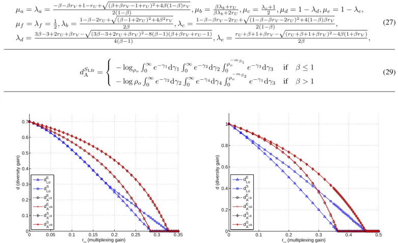
Fig. 3. The optimal DMT functions ofEandSin CSI-L,dLo(r), and the
lower and upper bounds of the DMT functions ofE andS in CSI-A with
rV = 32rUandβ= 0.7.
i−th user. The MMGs are the smallest rootsrU andrV of the
equationsd(rU, rV) = 0whered(rU, rV)is the corresponding
DMT function. The MMG pair including the MMGs of two users U and V is a curve represented by a certain equation
f(rU, rV) = 0. With the schemeEin CSI-L, the MMGs satisfy
rU,ELo= 1−θo(rEU,Lo, r E
V,Lo)whereθo is given in Proposition
4.2. The equation gives rE
V,Lo = 1−2r E
U,Lo which is also
simmilar to the equation for MMGs of scheme E in CSI-A rE
V,Ao= 1−2rEU,Ao. For the schemeS in CSI-L, the MMGs
satisfyrS
U,Lo= 1−µj(rSU,Lo, rSV,Lo),j∈ {a, b, ..., f}ifβ ≤1
andrSU,Lo= 1−λj(rSU,Lo, r S
V,Lo)and ifβ >1, whereµj and
λj are given in Proposition 4.5. The equations give
rSV,Ao=
( 1−2rU
β if β≤1
1−1 + 1
β
rU if β >1.
(30)
which are also the equations for MMGs of schemeS in CSI-A. Clearly, the MMGs of schemeS are larger than MMGs of schemeE.
V. NUMERICALRESULTS
The following numerical results show the DMT functions of scheme S and E in the two models CSI-L and CSI-A. In the CSI-L model, dEL and dSL are functions of (λ, θ) and
(λ, µ) respectively, dELo and dSLo are the optimal functions when optimized with respect to (λ, θ)and(λ, µ)respectively.
0 0.1 0.2 0.3 0.4 0.5 0
0.2 0.4 0.6 0.8 1
r
U (multiplexing gain)
d
(
d
iv
e
rs
it
y
g
a
in
)
dE Lo dS
Lo dELB
A dEUB
A dSLB
A dSUB
A
Fig. 4. The optimal DMT functions ofEandSin CSI-L,dLo(r), and the
lower and upper bounds of the DMT functions ofE andSin CSI-A with
rV =34rUandβ= 2.3.
In the CSI-A model, the lower bounds of the DMT functions of schemes E and S are numerically calculated with large enoughρ=ρo. In both cases of β≤1 andβ >1, the lower
bounds are quite close to their corresponding upper bounds. In Fig. 3, the DMT functions of schemeS andE in CSI-L and CSI-A are shown for the case with rV = 32rU and
β = 0.7. In case of β >1, by a similar variable substitution, we can see a similar comparison between dS
L and dEL. For
CSI-A, the results withβ= 2.3 andrV = 34rU are shown in
Fig. 4. From (6), (11), (19), (20) and (28), we observe that all schemes have the same maximum diversity gain ofmin(1, β), regardless of the CSI model.
The reference scheme gives the same MMG for both CSI-L and CSI-A channel models. The CDR scheme also has the same MMG for both CSI models but with a different value with the reference scheme. Therefore, at higher multiplexing gains, knowing all channels does not help significantly while applying the CDR scheme gives a significant improvement as shown in Fig. 3 and 4. At lower multiplexing gains, knowing all channels brings a large gain while applying the CDR scheme does not give a significant improvement.
(
minn(1−µ) log(1 +ργ1),(µ−λ) log(1 +ργ2) +λ
1 + ργ2
ρβγ
4+1 o
≥ rUlogρ
λlog(1 +ρβγ
3) ≥ rV logρβ
(31)
0 0.5 1 1.5 2 2.5 3 0
0.1 0.2 0.3 0.4 0.5 0.6 0.7 0.8
β
d
iv
e
rs
it
y
g
a
in
dEL
dSL
dEUB
A dSUB
A dELB
A dSLB
A
Fig. 5. The optimal DMT functions in CSI-L,dLo(r), ofEandSand the
lower and upper bounds of the DMT functions ofE andS in CSI-A with fixedrU=rV = 0.2.
0 0.5 1 1.5 2 2.5 3 0.2
0.3 0.4 0.5 0.6 0.7 0.8 0.9
β
o
p
ti
m
a
l
d
u
ra
ti
o
n
θE o λE o µS o λS o
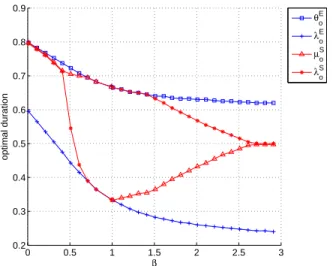
Fig. 6. The optimized tranmissions durations of schemeE (θandλ) and schemeS(µandλ) in CSI-L with fixedrU=rV = 0.2.
as the desired signal thus both NIC or IC options consisting in treating interference as noise or decoding and cancelling it are not efficient. This also holds for CSI-L. The difference between CSI-L and CSI-A achieves its maximum at β = 1. Thus knowing all channels benefits the most when β = 1. These are reflected in Fig. 5 with a multiplexing gain rfixed at 0.2.
The optimized DMT function of scheme E in CSI-L is given by a single expression in Proposition 4.2 while the optimized DMT function of scheme S in CSI-L is given by many expressions for cases of β Proposition 4.5. Therefore as shown in Fig. 6 where the optimal µ and λof scheme S andEin CSI-L are shown also with fixedr= 0.2and varied β, there are several corresponding discontinuities in case of
schemeS.
Regarding the limit of the diversity gain when β tends to infinity, as shown in Fig. 5, increasing β over 1 does not give any improvement for scheme E in CSI-A. The reason is that its diversity gain reaches and not affected by β as seen in (11). On the other hand for scheme S in CSI-A, the
limit is higher at limβ→∞dSAU B =
1−rU−rV 1−rV
+
= 0.75.
For scheme E in CSI-L, a very high β means a very high dEV = β(1− rV
λ)
+ in (6). The diversity gain of the scheme
dEL = mindEU1, dEU2, dEV is hence limited by dEU1 and dEU2
which corresponds to transmission duration ratios 1−θ and θ−λ. Thereforeλshould be reduced as much as possible to make1−θandθ−λhigher. However,λmust be kept larger than or equal torV =rto make 1−rλV
not negative. Hence the optimal value is λo = rV = 0.2. The optimal θ can be
calculated based on equation dE U1 =d
E
U2 which is equivalent to 1−µ =µ−λ from which we obtain µo = 1+2rV = 0.6
thereforelimβ→∞dEL = 1−
0.2
1−0.4 = 0.5as seen in the figure.
The case with schemeSin CSI-L is dealt similarly. The limit of diversity gain of scheme S is higher than that of scheme E.
VI. CONCLUSION
In this paper, we have considered a network with a base station, a relay station, a relayed user and a direct user in two models with different channel knowledge levels. The Diversity-Multiplexing Trade-off (DMT) functions of the Co-ordinated Direct and Relay (CDR) scheme and of the corre-sponding conventional scheme are either analytically calcu-lated or bounded. The transmission durations in both schemes are optimized accordingly. The results reveal that at low diversity gains, knowledge of all channels at a station does not improve the DMT function. Nevertheless, upgrading the conventional scheme to the CDR scheme brings improvement in terms of the multiplexing gain. Conversely, at high diversity gains, upgrading does not help while knowing all channels can improve the DMT function.
APPENDIX
PROOF OFPROPOSITION4.6
We consider the two casesβ ≤1 andβ≥1.
A. β ≤1
Similarly to the CSI-L case, we considerµ≥λ. From the expressions for RS
U1, R
S
U2 and R
S
V, we derive the condition
for no outage as in (31). It is equivalent to
µ≤1−a1, λ≥a3 and µ≥max(λ(1−a4) +a2, λ)
(36) with a1, a2 and a3 as denoted in section IV-B2 and a4 =
log1+ ργ2
ρβ γ4 +1
PrhOS2
A
i
= Prh rU
1−α1 +
rU 1−α2 +
βrV 1−α3
β
>1i
= Pr
βα1+βα2+α3−βα1(rU+βrV)−βα2(rU+βrV)−2α3rU > β−2βrU−β2rV
.
≥Pr
α3−2α3rU > β−2βrU−β2rV
= Prhα3> β1−21r−U2−rUβrV
i .
=ρ−β
(1−2rU−βrV)
1−2rU +
(32)
(
min
(1−λ) log(1 +ργ1), µlog(1 +ρβγ2) ≥ rUlogρ
minn(λ−µ) log(1 +ρβγ
4) +µ
1 + ρβγ4
ργ2+1
, λlog(1 +ρβγ
3)
o
≥ rV logρβ
(33)
PrhOS2
A
i
= Prh rU
1−α1 +
rV 1−α4
β
+ rU
β(1−α2) >1 i
.
= Prhα1(β−βrV −rU) +α2(β−βrU−βrV) +α4(1−rU−rβU)> β−βrU −βrV −rU
i
.
≥Pr [α1(β−βrV −rU)> β−βrU −βrV −rU] = Pr
h
α1> β−(ββ−+1)r rU−βrV U−βrV
i . ≥ρ
− 1−(1+ 1β)rU−rV 1−rUβ−rV
!+ (34)
Pr
OS
A
.
= PrhOS1
A
i
+ PrhOS2
A
i
+ PrhOS3
A
i
.
= max
ρ− 1−2rU
1−rU +
, ρ−β
1−rU−rV
1−rU +
, ρ
− 1−(1+ 1β)rU−rV 1−rU
β −rV
!+
=ρ
− 1−(1+ 1β)rU−rV 1−rU
β−rV !+
(35)
λ µ
a2
1– a1
µ = λ(1 – a4) + a2 a
2/a4
µ = λ
λ a2
µ = λ λ= a5+ (1 – a6)µ
a3
λ
O a3
λ O 1 – a1
(a) β ≤ 1 and µ ≥λ
a6
(b) β> 1 and µ < λ
Fig. 7. Non-outage areas forµ≥λandµ < λin CDRS.
7a. Using the method in section IV-B2, we can derive that (36) never occurs if the point (a3,1−a1) lies below one of
the lines µ=λ andµ =λ(1−a4) +a2 or 1−a1 < b1 =
max(a2+a3(1−a4), a3). In this case, we cannot find any
(λ, µ) to accommodate the target rate pair. The condition is equivalent to OS
A=O
S1
A ∪ O
S2
A whereO
S1
A ,{1−a1< a3}
andOS2
A ,{1−a1< a2+a3(1−a4)}. Similarly to schemeE
in CSI-A, we have PrhOS1
A
i . ≥ρ−β
1−rU−rV
1−rU +
,dS1
A. On
the other hand, becauselimρ→∞a4= 1−β, we have (32).
Pr
OS
A
.
= PrhOS1
A
i
+ PrhOS2
A
i
.
= max
ρ−β
1−rU−rV
1−rU +
, ρ−β
(1−2rU−βrV) 1−2rU
+
=ρ−β
(1−2rU−βrV) 1−2rU
+
.
(37)
The DMT function is therefore given in (28).
B. β >1
We consider µ < λ. The condition for no outage is given in (33). It is equivalent to
λ≤1−a1, µ≥a2,
λ≥max(µ(1−a5) +a6, µ), λ≥a3
(38)
with a1, a2, a3 as denoted in section IV-B2, a5 = log
1+ρβ γ4
ργ2 +1
log(1+ρβγ
4) and a6 =
log(1+ρβ)
log(1+ρβγ
4). The no-outage area is demonstrated in Fig. 7b. Using the method in section IV-B2, we can see that (38) never occurs if (1) the point
(a3,1−a1) lies above one of the lines λ = µ and λ = µ(1 − a5) +a6 or (2) a3 < 1 − a1. The condition is
equivalent to 1−a1 < max(a2, a6+a2(1−a5), a3). The
outage condition is denoted asOS
A=O
S1
A ∪ O
S2
A ∪ O
S3
A where
OS1
A , [1−a1 < a2], OAS2 , [1−a1 < a6+a2(1−a5)]
andOS3
A ,[1−a1< a3]in which Pr
h OS1
A
i .
=ρ−
1−2rU
1−rU +
andPrhOS3
A
i .
=ρ−β
1−rU−rV
1−rU +
. On the other hand, because
limρ→∞a5= 1−β1, we have (34) and (35). The upper bound
of the DMT function in this case is therefore given in (28).
REFERENCES
[1] G. Farhadi and N. C. Beaulieu, “Capacity of amplify-and-forward multi-hop relaying systems under adaptive transmission,” IEEE Trans. on Comm., vol 58, iss. 3, pp 758-763, 2010.
[2] Y. Zhu, P.-Y. Kam, and Y. Xin, “Differential modulation for decode-and-forward multiple relay systems,”IEEE Trans. on Comm., vol 58, iss. 1, pp. 189-199, 2010.
[4] C. Thai, P. Popovski, M. Kaneko and E. Carvalho, “Multi-flow scheduling for coordinated direct and relayed users in cellular systems,”IEEE Trans. on Comm., Jan 2013.
[5] P. Popovski and H. Yomo, “Bi-directional amplification of throughput in a wireless multi–hop network,” inProc. IEEE VTC, Spring 2006. [6] S. Katti, S. Gollakota, and D. Katabi “Embracing wireless interference:
Analog network coding,” inProc. ACM SIGCOMM, 2007.
[7] H. Ning, C. Ling, and K. K. Leung, “Wireless network coding with imperfect overhearing,” arXiv:1003.4270v1 [cs.IT], 22 Mar 2010. [8] F. Sun, T. M. Kim, A. J. Paulraj, E. de Carvalho, and P. Popovski,
“Cell-Edge Multi-User Relaying with Overhearing,”IEEE Commun. Lett., 2013. [9] F. Sun, E. de Carvalho, P. Popovski and C. Thai, “Coordinated Direct and Relay Transmission with Linear Non-Regenerative Relay Beamforming,”
IEEE Signal Process. Lett., vol. 19, no. 10, Oct. 2012.
[10] C. Thai and P. Popovski, “Coordinated direct and relay transmission with interference cancelation in wireless systems,”IEEE Comm. Letters, vol. 15, no. 4, Apr 2011, pp. 416-418
[11] C. Thai, P. Popovski, M. Kaneko and E. Carvalho, “Coordinated transmissions to direct and relayed users in wireless cellular systems,” inProc. IEEE ICC, Kyoto, Japan, Jun 2011.
[12] C. Thai and P. Popovski, “Coordination of regenerative relays and direct users in wireless Cellular Networks,” inProc. IEEE ISWCS’11, Aachen, Germany, Nov 2011.
[13] L. Zheng and D. N. C. Tse, “Diversity and multiplexing: A fundamental tradeoff in multiple antenna channels,”IEEE Trans. Inform. Theory, vol. 49, pp. 1073-1096, May 2003.
[14] T. Kim and H. Poor, “Diversity-multiplexing trade-off in adaptive two-way relaying,”IEEE Trans. on Info. Theo., vol. 57, iss. 7, pp. 4235 -4254, June 2011.
[15] D. Tse and R. Viswanath, “Fundamentals of wireless Communications,” Chap. 8, Cambridge Press, 2005.
[16] M. Ansari, A. Bayesteh and A. Khandani, “Diversity-multiplexing trade-off in Z-channel,” inProc. IEEE CWIT, pp. 21-24, June 2007. [17] E. Akuiyibo and O. Leveque, “Diversity-multiplexing tradeoff for the
slow fading interference Channel,” inProc. in IEEE IZS, pp. 140 - 143, Mar. 2008.
[18] M. Yuksel and E. Erkip, “Diversity-multiplexing tradeoff for MIMO wire-tap channels with CSIT,” inProc. IEEE EW, pp. 796 - 801, June 2010.
Chan Dai Truyen Thaireceived his B.S. from Posts and Telecommunications Institute of Technology, Vietnam, in 2003, his MSc. from Korea Advanced Institute of Science and Technology (KAIST), South Korea, in 2008 and Ph.D. from Aalborg Univer-sity, Denmark, in 2012. He is now a postdoc-toral researcher in IFSTTAR, LEOST, Villeneuve d’Ascq, France. His interest topics include: coopera-tive/relaying communications, femtocell, vehicle-to-vehicle communications, communication for high-speed vehicles.
Petar Popovski (S’97–A’98–M’04–SM’10) re-ceived Dipl.-Ing. in electrical engineering (1997) and Magister Ing. in communication engineering (2000) from Sts. Cyril and Methodius University, Skopje, Macedonia, and Ph. D. from Aalborg University, Denmark, in 2004. He is currently a Professor at Aalborg University. He has more than 160 publica-tions in journals, conference proceedings and books and has more than 25 patents and patent applications. He has received the Young Elite Researcher award and the SAPERE AUDE career grant from the Danish Council for Independent Research. He has received six best paper awards, including three from IEEE. Dr. Popovski serves on the editorial board of several journals, including IEEE Communications Letters (Senior Editor), IEEE JSAC Cognitive Radio Series, and IEEE Transactions on Communications. He is a Steering Committee member for the upcoming IEEE Transactions on Internet of Things and Chair of the ComSoc subcommittee on Smart Grid Communications. His research interests are in the broad area of wireless communication and networking, information theory and protocol design.
Elisabeth de Carvalho received a Ph.D. in elec-trical engineering from Telecom ParisTech, France, in 1999. After her Ph.D, she was a post-doctoral fellow at Stanford University working in the field of ADSL communications. Then she worked in industry in the field of ADSL and wireless LAN. She joined Aalborg University in 2005 where she has led several national and international research projects in wireless communications. Her general area of expertise is in digital signal processing for wireless communications with multiple antennas. She is a co-author of the text book “A Practical Guide to the MIMO Radio Channel.”