NBER WORKING PAPER SERIES
SYSTEMIC RISK AND HEDGE FUNDS Nicholas Chan Mila Getmansky Shane M. Haas Andrew W. Lo Working Paper11200 http://www.nber.org/papers/w11200
NATIONAL BUREAU OF ECONOMIC RESEARCH 1050 Massachusetts Avenue
Cambridge, MA 02138 March 2005
Prepared for the NBER Conference on the Risks of Financial Institutions. The views and opinions expressed in this article are those of the authors only, and do not necessarily represent the views and opinions of AlphaSimplex Group, MIT, the University of Massachusetts, or any of their affiliates and employees. The authors make no representations or warranty, either expressed or implied, as to the accuracy or completeness of the information contained in this article, nor are they recommending that this article serve as the basis for any investment decision|this article is for information purposes only. Research support from AlphaSimplex Group and the MIT Laboratory for Financial Engineering is gratefully acknowledged. We thank David Modest and participants of the NBER Conference on The Risks of Financial Institutions for helpful comments and discussion. Parts of this paper include ideas and exposition from several previously published papers and books of some of the authors. Where appropriate, we have modi ed the passages to suit the current context and composition without detailed citations and quotation marks so as preserve continuity. Readers interested in the original sources of those passages should consult Getmansky (2004), Getmansky, Lo, and Makarov (2004), Getmansky, Lo, and Mei (2004), and Lo (2001, 2002). The views expressed herein are those of the author(s) and do not necessarily reflect the views of the National Bureau of Economic Research.
© 2005 by Nicholas Chan, Mila Getmansky, Shane M. Haas, and Andrew W. Lo. All rights reserved. Short sections of text, not to exceed two paragraphs, may be quoted without explicit permission provided that full credit, including © notice, is given to the source.
Systemic Risk and Hedge Funds
Nicholas Chan, Mila Getmansky, Shane M. Haas, and Andrew W. Lo NBER Working Paper No. 11200
March 2005 JEL No. G12
ABSTRACT
Systemic risk is commonly used to describe the possibility of a series of correlated defaults among financial institutions---typically banks---that occur over a short period of time, often caused by a single major event. However, since the collapse of Long Term Capital Management in 1998, it has become clear that hedge funds are also involved in systemic risk exposures. The hedge-fund industry has a symbiotic relationship with the banking sector, and many banks now operate proprietary trading units that are organized much like hedge funds. As a result, the risk exposures of the hedge-fund industry may have a material impact on the banking sector, resulting in new sources of systemic risks. In this paper, we attempt to quantify the potential impact of hedge funds on systemic risk by developing a number of new risk measures for hedge funds and applying them to individual and aggregate hedge-fund returns data. These measures include: illiquidity risk exposure, nonlinear factor models for hedge-fund and banking-sector indexes, logistic regression analysis of hedge-fund liquidation probabilities, and aggregate measures of volatility and distress based on regime-switching models. Our preliminary findings suggest that the hedge-fund industry may be heading into a challenging period of lower expected returns, and that systemic risk is currently on the rise. Nicholas Chan
AlphaSimplex Group, LLC One Cambridge Center Cambridge, MA 0214 [email protected] Mila Getmansky
Isenberg School of Management University of Massachusetts Amherst, MA 01003
Shane M. Haas
AlphaSimplex Group, LLC One Cambridge Center Cambridge, MA 02142 [email protected] Andrew W. Lo
MIT Sloan School of Management 50 Memorial Drive, E52-432 Cambridge, MA 02142 and NBER
Contents
1 Introduction 1 1.1 Tail Risk . . . 6 1.2 Phase-Locking Risk . . . 13 2 Literature Review 17 3 The Data 20 3.1 CSFB/Tremont Indexes . . . 23 3.2 TASS Data . . . 284 Measuring Illiquidity Risk 36 4.1 Serial Correlation and Illiquidity . . . 37
4.2 An Econometric Model of Smoothed Returns . . . 41
4.3 Maximum Likelihood Estimates of Smoothing Profiles . . . 47
4.4 An Aggregate Measure of Illiquidity . . . 54
5 Hedge-Fund Liquidations 56 5.1 Attrition Rates . . . 61
5.2 Logit Analysis of Liquidations . . . 66
6 Other Hedge-Fund Measures of Systemic Risk 79 6.1 Risk Models for Hedge Funds . . . 80
6.2 Hedge Funds and the Banking Sector . . . 87
6.3 Regime-Switching Models . . . 90
7 The Current Outlook 97 A Appendix 98 A.1 TASS Category Definitions . . . 98
1
Introduction
The term “systemic risk” is commonly used to describe the possibility of a series of correlated defaults among financial institutions—typically banks—that occurs over a short period of time, often caused by a single major event. A classic example is a banking panic in which large groups of depositors decide to withdraw their funds simultaneously, creating a run on bank assets that can ultimately lead to multiple bank failures. Banking panics were not uncommon in the U.S. during the nineteenth and early twentieth centuries, culminating in the 1930–1933 period with an average of 2,000 bank failures per year during these years according to Mishkin (1997), and which prompted the Glass-Steagall Act of 1933 and the establishment of the Federal Deposit Insurance Corporation in 1934.
Although today banking panics are virtually non-existent thanks to the FDIC and related central banking policies, systemic risk exposures have taken shape in other forms. With the repeal in 1999 of the Glass-Steagall Act, many banks have now become broad-based finan-cial institutions engaging in the full spectrum of finanfinan-cial services including retail banking, underwriting, investment banking, brokerage services, asset management, venture capital, and proprietary trading. Accordingly, the risk exposures of such institutions have become considerably more complex and interdependent, especially in the face of globalization and the recent wave of consolidations in the banking and financial services sectors.
In particular, innovations in the banking industry have coincided with the rapid growth of hedge funds, unregulated and opaque investment partnerships that engage in a variety
of active investment strategies, often yielding double-digit returns and commensurate risks.1
Currently estimated at over $1 trillion in size, the hedge fund industry has a symbiotic rela-tionship with the banking sector, providing an attractive outlet for bank capital, investment management services for banking clients, and fees for brokerage services, credit, and other banking functions. Moreover, many banks now operate proprietary trading units which are organized much like hedge funds. As a result, the risk exposures of the hedge-fund industry may have a material impact on the banking sector, resulting in new sources of systemic
risks. And although many hedge funds engage in hedged strategies—where market swings
are partially or completely offset through strategically balanced long and short positions in various securities—such funds often have other risk exposures such as volatility risk, credit risk, and liquidity risk. Moreover, many hedge funds are not hedged at all, and also use
1
Although hedge funds have avoided regulatory oversight in the past by catering only to “qualified” investors (investors that meet a certain minimum threshold in terms of net worth and investment experience) and refraining from advertising to the general public, a recent ruling by the U.S. Securities and Exchange Commission (Rule 203(b)(3)–2) will require most hedge funds to register as investment advisers under the Investment Advisers Act of 1940 by February 1, 2006.
leverage to enhance their returns and, consequently, their risks.
In this paper, we attempt to quantify the potential impact of hedge funds on systemic risk by developing a number of new risk measures for hedge-fund investments and applying them to individual and aggregate hedge-fund returns data. We argue that the risk/reward profile for most alternative investments differ in important ways from more traditional investments, and such differences may have potentially important implications for systemic risk, as we experienced during the aftermath of the default of Russian government debt in August 1998 when Long Term Capital Management and many other hedge funds suffered catastrophic losses over the course of a few weeks, creating significant stress on the global financial system and a number of substantial financial institutions. Two major themes emerged from that set of events: the importance of liquidity and leverage, and the capriciousness of correlations among instruments and portfolios that are supposedly uncorrelated. These are the two main themes of this study, and both are intimately related to the dynamic nature of hedge-fund investment strategies and risk exposures.
One of the justifications for the unusually rich fee structures that characterize hedge-fund investments is the fact that hedge funds are active strategies involving highly skilled portfolio managers. Moreover, it is common wisdom that the most talented managers are drawn first to the hedge-fund industry because the absence of regulatory constraints enables them to make the most of their investment acumen. With the freedom to trade as much or as little as they like on any given day, to go long or short any number of securities and with varying degrees of leverage, and to change investment strategies at a moment’s notice, hedge-fund managers enjoy enormous flexibility and discretion in pursuing performance. But dynamic investment strategies imply dynamic risk exposures, and while modern financial economics
has much to say about the risk of static investments—the market beta is sufficient in this
case—there is currently no single measure of the risks of a dynamic investment strategy.2
These challenges have important implications for both managers and investors since both parties seek to manage the risk/reward trade-offs of their investments. Consider, for example, the now-standard approach to constructing an optimal portfolio in the mean-variance sense:
Max{ωi}E[U(W1)] (1) subject to W1 = W0(1 +Rp) (2a) Rp ≡ n X i=1 ωiRi , 1 = n X i=1 ωi (2b) 2
For this reason, hedge-fund track records are often summarized with multiple statistics, e.g., mean, standard deviation, Sharpe ratio, market beta, Sortino ratio, maximum drawdown, worst month, etc.
where Ri is the return of security i between this period and the next, W1 is the
indi-vidual’s next period’s wealth (which is determined by the product of the {Ri} with the
portfolio weights {ωi}), andU(·) is the individual’s utility function. By assuming thatU(·)
is quadratic, or by assuming that individual security returns Ri are normally distributed
random variables, it can be shown that maximizing the individual’s expected utility is
tan-tamount to constructing a mean-variance optimal portfolioω∗.3
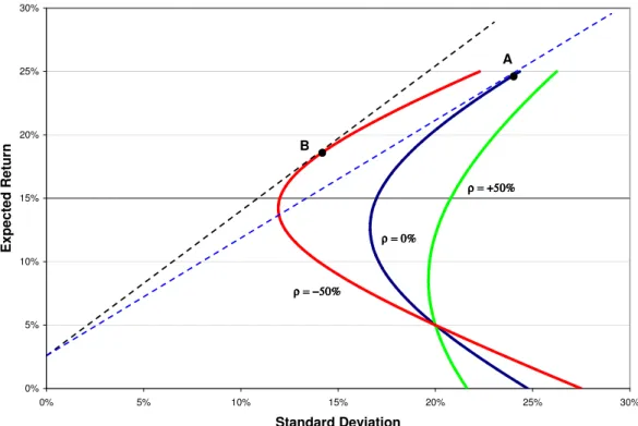
It is one of the great lessons of modern finance that mean-variance optimization yields benefits through diversification, the ability to lower volatility for a given level of expected return by combining securities that are not perfectly correlated. But what if the securities are hedge funds, and what if their correlations change over time, as hedge funds tend to do
(see Section 3.1)?4 Table 1 shows that for the two-asset case with fixed means of 5% and 30%,
respectively, and fixed standard deviations of 20% and 30%, respectively, as the correlation
ρ between the two assets varies from −90% to 70%, the optimal portfolio weights—and
the properties of the optimal portfolio—change dramatically. For example, with a −30%
correlation between the two funds, the optimal portfolio holds 38.6% in the first fund and
61.4% in the second, yielding a Sharpe ratio of 1.01. But if the correlation changes to 10%,
the optimal weights change to 5.2% in the first fund and 94.8% in the second, despite the
fact that the Sharpe ratio of this new portfolio, 0.92, is virtually identical to the previous portfolio’s Sharpe ratio. The mean-variance-efficient frontiers are plotted in Figure 1 for
three values of the correlation coefficient between the two funds (−50%, 0%, and 50%), and
it is apparent that the optimal portfolio depends heavily on this correlation. For example,
as the correlation between the two assets changes from 0% to −50%, the optimal portfolio
changes from A to B, which are two very different portfolios. Because of the dynamic nature of hedge-fund strategies, their correlations are particularly unstable through time and over
varying market conditions as we shall see in Section 1.2, and swings from −30% to 30% are
not unusual.
Table 1 shows that as the correlation between the two assets increases, the optimal weight for asset 1 eventually becomes negative, which makes intuitive sense from a hedging perspective even if it is unrealistic for hedge-fund investments and other assets that cannot be shorted. Note that for correlations of 80% and greater, the optimization approach does not yield a well-defined solution because a mean-variance-efficient tangency portfolio does not exist for the parameter values we hypothesized for the two assets. However, numerical
3
See, for example, Ingersoll (1987).
4
Several authors have considered mean-variance optimization techniques for determining hedge-fund al-locations, with varying degrees of success and skepticism. See, in particular, Amenc and Martinelli (2002), Amin and Kat (2003c), Terhaar, Staub, and Singer (2003), and Cremers, Kritzman, and Page (2004).
Mean-Variance Optimal Portfolios For Two-Asset Case
(µ1, σ1) = (5%,20%), (µ2, σ2) = (30%,30%), Rf = 2.5% ρ E[R∗] SD[R∗] Sharpe ω∗ 1 ω∗2 −90 15.5 5.5 2.36 58.1 41.9 −80 16.0 8.0 1.70 55.9 44.1 −70 16.7 10.0 1.41 53.4 46.6 −60 17.4 11.9 1.25 50.5 49.5 −50 18.2 13.8 1.14 47.2 52.8 −40 19.2 15.7 1.06 43.3 56.7 −30 20.3 17.7 1.01 38.6 61.4 −20 21.8 19.9 0.97 32.9 67.1 −10 23.5 22.3 0.94 25.9 74.1 0 25.8 25.1 0.93 17.0 83.0 10 28.7 28.6 0.92 5.2 94.8 20 32.7 32.9 0.92 −10.9 110.9 30 38.6 38.8 0.93 −34.4 134.4 40 48.0 47.7 0.95 −71.9 171.9 50 65.3 63.2 0.99 −141.2 241.2 60 108.1 99.6 1.06 −312.2 412.2 70 387.7 329.9 1.17 −1430.8 1530.8
Table 1: Mean-variance optimal portfolio weights for the two-asset case with fixed means
0% 5% 10% 15% 20% 25% 30% 0% 5% 10% 15% 20% 25% 30% Standard Deviation E xp ec te d R et ur n ρ = 0% ρ = 0% ρ = 0% ρ = 0% ρ = −50% ρ = −50% ρ = −50% ρ = −50% ρ = +50% ρ = +50% ρ = +50% ρ = +50% A B
Figure 1: Mean-variance efficient frontiers for the two-asset case with parameters (µ1, σ1) =
optimization procedures may still yield a specific portfolio for this case, e.g., a portfolio on the lower branch of the mean-variance parabola, even if it is not optimal. This example underscores the importance of modeling means, standard deviations, and correlations in a consistent manner when accounting for changes in market conditions and statistical regimes, otherwise degenerate or nonsensical “solutions” may arise.
To illustrate the challenges and opportunities in modeling the risk exposures of hedge funds, we provide two concrete examples in this section. In Section 1.1, we present a hy-pothetical hedge-fund strategy that yields remarkable returns with seemingly little risk, yet a closer examination will reveal quite a different story. And in Section 1.2, we show that correlation analysis may not be able capture certain risk exposures that are particularly relevant for hedge-fund investments.
These examples provide an introduction to the analysis in Sections 3–7, and serve as motivation for developing new quantitative methods for capturing the impact of hedge funds on systemic risk. In Section 3, we summarize the empirical properties of aggregate and individual hedge fund data used in this study, the CSFB/Tremont hedge-fund indexes and the TASS individual hedge-fund database. In Section 4, we turn to the issue of liquidity—one of the central aspects of systemic risk—and present several measures for gauging illiquidity exposure in hedge funds and other asset classes, and apply them to individual and index data. Since systemic risk is directly related to hedge-fund failures, in Section 5 we investigate attrition rates of hedge funds in the TASS database and present a logit analysis that yields estimates of a fund’s probability of liquidation as a function of various fund characteristics such as return history, assets under management, and recent fund flows. In Section 6, we present three other approaches to measuring systemic risk in the hedge-fund industry: risk models for hedge-fund indexes, regression models relating the banking sector to hedge funds, and regime-switching models applied to hedge-fund indexes. These three approaches yield distinct insights regarding the risks posed by the hedge-fund industry, and we conclude in Section 7 by discussing the current outlook for the hedge-fund industry based on the analytics and empirical results of this study. Our tentative inferences suggest that the hedge-fund industry may be heading into a challenging period of lower expected returns, and that systemic risk has been increasing steadily over the recent past.
1.1
Tail Risk
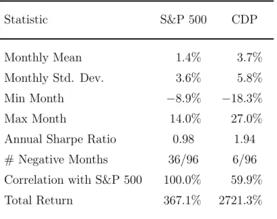
Consider the 8-year track record of a hypothetical hedge fund, Capital Decimation Partners, LP, summarized in Table 2. This track record was obtained by applying a specific investment strategy, to be revealed below, to actual market prices from January 1992 to December 1999.
Before discussing the particular strategy that generated these results, let us consider its overall performance: an average monthly return of 3.7% versus 1.4% for the S&P 500 during
the same period; a total return of 2,721.3% over the 8-year period versus 367.1% for the S&P
500; a Sharpe ratio of 1.94 versus 0.98 for the S&P 500; and only 6 negative monthly returns out of 96 versus 36 out of 96 for the S&P 500. In fact, the monthly performance history— displayed in Table 3—shows that, as with many other hedge funds, the worst months for this fund were August and September of 1998. Yet October and November 1998 were the fund’s two best months, and for 1998 as a whole the fund was up 87.3% versus 24.5% for the S&P 500! By all accounts, this is an enormously successful hedge fund with a track record
that would be the envy of most managers.5 What is its secret?
Capital Decimation Partners, L.P.
Performance Summary, January 1992 to December 1999
Statistic S&P 500 CDP
Monthly Mean 1.4% 3.7%
Monthly Std. Dev. 3.6% 5.8%
Min Month −8.9% −18.3%
Max Month 14.0% 27.0%
Annual Sharpe Ratio 0.98 1.94
# Negative Months 36/96 6/96
Correlation with S&P 500 100.0% 59.9%
Total Return 367.1% 2721.3%
Table 2: Summary of simulated performance of a particular dynamic trading strategy using monthly historical market prices from January 1992 to December 1999.
The investment strategy summarized in Tables 2 and 3 consists of shorting out-of-the-money S&P 500 (SPX) put options on each monthly expiration date for maturities less than or equal to three months, and with strikes approximately 7% out of the money. The num-ber of contracts sold each month is determined by the combination of: (1) CBOE margin
5
In fact, as a mental exercise to check your own risk preferences, take a hard look at the monthly returns in Table 3 and ask yourself whether you would invest in such a fund.
requirements;6 (2) an assumption that we are required to post 66% of the margin as
collat-eral;7 and (3) $10M of initial risk capital. For concreteness, Table 4 reports the positions
and profit/loss statement for this strategy for 1992. See Lo (2001) for further details of this strategy.
The track record in Tables 2 and 3 seems much less impressive in light of the simple strategy on which it is based, and few investors would pay hedge-fund-type fees for such a fund. However, given the secrecy surrounding most hedge-fund strategies, and the broad discretion that managers are given by the typical hedge-fund offering memorandum, it is difficult for investors to detect this type of behavior without resorting to more sophisticated
risk analytics that can capture dynamic risk exposures.
6
The margin required per contract is assumed to be:
100× {15%×(current level of the SPX)−(put premium)−(amount out of the money)}
where the amount out of the money is equal to the current level of the SPX minus the strike price of the put.
7
This figure varies from broker to broker, and is meant to be a rather conservative estimate that might apply to a $10M startup hedge fund with no prior track record.
Capital Decimation Partners, L.P.
Monthly Performance History
1992 1993 1994 1995 1996 1997 1998 1999 Month SPX CDP SPX CDP SPX CDP SPX CDP SPX CDP SPX CDP SPX CDP SPX CDP Jan 8.2 8.1 −1.2 1.8 1.8 2.3 1.3 3.7 −0.7 1.0 3.6 4.4 1.6 15.3 5.5 10.1 Feb −1.8 9.3 −0.4 1.0 −1.5 0.7 3.9 0.7 5.9 1.2 3.3 6.0 7.6 11.7 −0.3 16.6 Mar 0.0 4.9 3.7 3.6 0.7 2.2 2.7 1.9 −1.0 0.6 −2.2 3.0 6.3 6.7 4.8 10.0 Apr 1.2 3.2 −0.3 1.6 −5.3 −0.1 2.6 2.4 0.6 3.0 −2.3 2.8 2.1 3.5 1.5 7.2 May −1.4 1.3 −0.7 1.3 2.0 5.5 2.1 1.6 3.7 4.0 8.3 5.7 −1.2 5.8 0.9 7.2 Jun −1.6 0.6 −0.5 1.7 0.8 1.5 5.0 1.8 −0.3 2.0 8.3 4.9 −0.7 3.9 0.9 8.6 Jul 3.0 1.9 0.5 1.9 −0.9 0.4 1.5 1.6 −4.2 0.3 1.8 5.5 7.8 7.5 5.7 6.1 Aug −0.2 1.7 2.3 1.4 2.1 2.9 1.0 1.2 4.1 3.2 −1.6 2.6 −8.9 −18.3 −5.8 −3.1 Sep 1.9 2.0 0.6 0.8 1.6 0.8 4.3 1.3 3.3 3.4 5.5 11.5 −5.7 −16.2 −0.1 8.3 Oct −2.6 −2.8 2.3 3.0 −1.3 0.9 0.3 1.1 3.5 2.2 −0.7 5.6 3.6 27.0 −6.6 −10.7 Nov 3.6 8.5 −1.5 0.6 −0.7 2.7 2.6 1.4 3.8 3.0 2.0 4.6 10.1 22.8 14.0 14.5 Dec 3.4 1.2 0.8 2.9 −0.6 10.0 2.7 1.5 1.5 2.0 −1.7 6.7 1.3 4.3 −0.1 2.4 Year 14.0 46.9 5.7 23.7 −1.6 33.6 34.3 22.1 21.5 28.9 26.4 84.8 24.5 87.3 20.6 105.7
Table 3: Simulated performance history of a particular dynamic trading strategy using monthly historical market prices from January 1992 to December 1999.
Some might argue that this example illustrates the need for position transparency— after all, it would be apparent from the positions in Table 4 that the manager of Capital Decimation Partners is providing little or no value-added. However, there are many ways of implementing this strategy that are not nearly so transparent, even when positions are fully disclosed. For example, Table 5 reports the weekly positions over a six-month period in one of 500 securities contained in a second hypothetical fund, Capital Decimation Partners II. Casual inspection of the positions of this one security seem to suggest a contrarian trading strategy: when the price declines, the position in XYZ is increased, and when the price advances, the position is reduced. A more careful analysis of the stock and cash positions and the varying degree of leverage in Table 5 reveals that these trades constitute a so-called “delta-hedging” strategy, designed to synthetically replicate a short position in a 2-year European put option on 10,000,000 shares of XYZ with a strike price of $25 (recall that XYZ’s initial stock price is $40, hence this is a deep out-of-the-money put).
Shorting deep out-of-the-money puts is a well-known artifice employed by unscrupulous hedge-fund managers to build an impressive track record quickly, and most sophisticated investors are able to avoid such chicanery. However, imagine an investor presented with position reports such as Table 5, but for 500 securities, not just one, as well as a corresponding track record that is likely to be even more impressive than that of Capital Decimation
Partners, LP.8 Without additional analysis that explicitly accounts for the dynamic aspects
of the trading strategy described in Table 5, it is difficult for an investor to fully appreciate the risks inherent in such a fund.
In particular, static methods such as traditional mean-variance analysis cannot capture the risks of dynamic trading strategies like Capital Decimation Partners (note the impressive Sharpe ratio in Table 2). In the case of the strategy of shorting out-of-the-money put options on the S&P 500, returns are positive most of the time and losses are infrequent, but when they occur, they are extreme. This is a very specific type of risk signature that is not well-summarized by static measures such as standard deviation. In fact, the estimated standard deviations of such strategies tend to be rather low, hence a naive application of mean-variance analysis such as risk-budgeting—an increasingly popular method used by institutions to make allocations based on risk units—can lead to unusually large allocations to funds like Capital Decimation Partners. The fact that total position transparency does not imply risk transparency is further cause for concern.
This is not to say that the risks of shorting out-of-the-money puts are inappropriate for all
8
A portfolio of options is worth more than an option on the portfolio, hence shorting 500 puts on the individual stocks that constitute the SPX will yield substantially higher premiums than shorting puts on the index.
Capital Decimation Partners, LP Positions and Profit/Loss For 1992
S&P 500 # Puts Strike Price Expiration Margin Required Profits
Initial Capital+ Cumulative Profits Capital Available for Investments Return 12/20/91 387.04 new 2300 360 4.625 Mar-92 $6,069,930 $10,000,000 $6,024,096
1/17/92 418.86 mark to market 2300 360 1.125 Mar-92 $654,120 $805,000 $10,805,000 $6,509,036 8.1%
418.86 new 1950 390 3.250 Mar-92 $5,990,205
Total Margin $6,644,325
2/21/92 411.46 mark to market 2300 360 0.250 Mar-92 $2,302,070 $690,000
411.46 mark to market 1950 390 1.625 Mar-92 $7,533,630 $316,875 $11,811,875 $7,115,587 9.3%
411.46 liquidate 1950 390 1.625 Mar-92 $0 $0 $11,811,875 $7,115,587 411.46 new 1246 390 1.625 Mar-92 $4,813,796 Total Margin $7,115,866 3/20/92 411.30 expired 2300 360 0.000 Mar-92 $0 $373,750 411.30 expired 1246 390 0.000 Mar-92 $0 $202,475 411.30 new 2650 380 2.000 May-92 $7,524,675 $12,388,100 $7,462,711 4.9% Total Margin $7,524,675
4/19/92 416.05 mark to market 2650 380 0.500 May-92 $6,852,238 $397,500
416.05 new 340 385 2.438 Jun-92 $983,280 $12,785,600 $7,702,169 3.2%
Total Margin $7,835,518
5/15/92 410.09 expired 2650 380 0.000 May-92 $0 $132,500
410.09 mark to market 340 385 1.500 Jun-92 $1,187,399 $31,875
410.09 new 2200 380 1.250 Jul-92 $6,638,170 $12,949,975 $7,801,190 1.3%
Total Margin $7,825,569
6/19/92 403.67 expired 340 385 0.000 Jun-92 $0 $51,000
403.67 mark to market 2200 380 1.125 Jul-92 $7,866,210 $27,500 $13,028,475 $7,848,479 0.6%
Total Margin $7,866,210
7/17/92 415.62 expired 2200 380 0.000 Jul-92 $0 $247,500
415.62 new 2700 385 1.8125 Sep-92 $8,075,835 $13,275,975 $7,997,575 1.9%
Total Margin $8,075,835
8/21/92 414.85 mark to market 2700 385 1 Sep-92 $8,471,925 $219,375 $13,495,350 $8,129,729 1.7%
Total Margin $8,471,925
9/18/92 422.92 expired 2700 385 0 Sep-92 $0 $270,000 $13,765,350 $8,292,380 2.0%
422.92 new 2370 400 5.375 Dec-92 $8,328,891
Total Margin $8,328,891
10/16/92 411.73 mark to market 2370 400 7 Dec-92 $10,197,992 ($385,125)
411.73 liquidate 2370 400 7 Dec-92 $0 $0 $13,380,225 $8,060,377 -2.8%
411.73 new 1873 400 7 Dec-92 $8,059,425
Total Margin $8,059,425
11/20/92 426.65 mark to market 1873 400 0.9375 Dec-92 $6,819,593 $1,135,506 $14,515,731 $8,744,416 8.5%
426.65 new 529 400 0.9375 Dec-92 $1,926,089
Total Margin $8,745,682
12/18/92 441.20 expired 1873 400 0 Dec-92 $0 $175,594 $14,691,325 $8,850,196 1.2%
1992 Total Return: 46.9%
Table 4: Simulated positions and profit/loss statement for 1992 for a trading strategy that consists of shorting out-of-the-money put options on the S&P 500 once a month.
investors—indeed, the thriving catastrophe reinsurance industry makes a market in precisely this type of risk, often called “tail risk”. However, such insurers do so with full knowledge of the loss profile and probabilities for each type of catastrophe, and they set their capital reserves and risk budgets accordingly. The same should hold true for institutional investors of hedge funds, but the standard tools and lexicon of the industry currently provide only an incomplete characterization of such risks. The need for a new set of dynamic risk analytics specifically targeted for hedge-fund investments is clear.
Capital Decimation Partners II, L.P.
Weekly Positions in XYZ
Week Pt Position Value Financing
t ($) (Shares) ($) ($) 0 40.000 7,057 282,281 −296,974 1 39.875 7,240 288,712 −304,585 2 40.250 5,850 235,456 −248,918 3 36.500 33,013 1,204,981 −1,240,629 4 36.875 27,128 1,000,356 −1,024,865 5 36.500 31,510 1,150,101 −1,185,809 6 37.000 24,320 899,841 −920,981 7 39.875 5,843 232,970 −185,111 8 39.875 5,621 224,153 −176,479 9 40.125 4,762 191,062 −142,159 10 39.500 6,280 248,065 −202,280 11 41.250 2,441 100,711 −44,138 12 40.625 3,230 131,205 −76,202 13 39.875 4,572 182,300 −129,796 14 39.375 5,690 224,035 −173,947 15 39.625 4,774 189,170 −137,834 16 39.750 4,267 169,609 −117,814 17 39.250 5,333 209,312 −159,768 18 39.500 4,447 175,657 −124,940 19 39.750 3,692 146,777 −95,073 20 39.750 3,510 139,526 −87,917 21 39.875 3,106 123,832 −71,872 22 39.625 3,392 134,408 −83,296 23 39.875 2,783 110,986 −59,109 24 40.000 2,445 97,782 −45,617 25 40.125 2,140 85,870 −33,445
Table 5: Simulated weekly positions in XYZ for a particular trading strategy over a six-month period.
1.2
Phase-Locking Risk
One of the most compelling reasons for investing in hedge funds is the fact that their returns seem relatively uncorrelated with market indexes such as the S&P 500, and modern portfolio theory has convinced even the most hardened skeptic of the benefits of diversification (see, for example, the correlations between hedge-fund indexes and the S&P 500 in Table 7 below). However, the diversification argument for hedge funds must be tempered by the lessons of the summer of 1998 when the default in Russian government debt triggered a global flight to quality that changed many of these correlations overnight from 0 to 1. In the physical and natural sciences, such phenomena are examples of “phase-locking” behavior, situations in
which otherwise uncorrelated actions suddenly become synchronized.9 The fact that market
conditions can create phase-locking behavior is certainly not new—market crashes have been with us since the beginning of organized financial markets—but prior to 1998, few hedge-fund investors and managers incorporated this possibility into their investment processes in any systematic fashion.
From a financial-engineering perspective, the most reliable way to capture phase-locking effects is to estimate a risk model for returns in which such events are explicitly allowed. For example, suppose returns are generated by the following two-factor model:
Rit = αi + βiΛt + ItZt + it (3)
and assume that Λt, It, Zt, and it are mutually independently and identically distributed
(IID) with the following moments:
E[Λt] = µλ , Var[Λt] = σλ2
E[Zt] = 0 , Var[Zt] = σz2
E[it] = 0 , Var[it] = σi2
(4)
and let the phase-locking event indicator It be defined by:
It = 1 with probability p 0 with probability 1−p . (5) 9
One of the most striking examples of phase-locking behavior is the automatic synchronization of the flickering of Southeast Asian fireflies. See Strogatz (1994) for a description of this remarkable phenomenon as well as an excellent review of phase-locking behavior in biological systems.
According to (3), expected returns are the sum of three components: the fund’s alpha, αi,
a “market” component, Λt, to which each fund has its own individual sensitivity, βi, and a
phase-locking component that is identical across all funds at all times, taking only one of two
possible values, either 0 (with probabilityp) orZt (with probability 1−p). If we assume that
pis small, say 0.001, then most of the time the expected returns of fundiare determined by
αi+βiΛt, but every once in a while an additional term Zt appears. If the volatilityσz of Zt
is much larger than the volatilities of the market factor, Λt, and the idiosyncratic risk, it,
then the common factor Zt will dominate the expected returns of all stocks whenIt= 1, i.e.,
phase-locking behavior.
More formally, consider theconditional correlation coefficient of two fundsiandj, defined
as the ratio of the conditional covariance divided by the square root of the product of the
conditional variances, conditioned on It= 0:
Corr[Rit, Rjt |It = 0] = βiβjσλ2 q β2 iσλ2 +σi2 q β2 jσ2λ+σj2 (6) ≈ 0 for βi ≈βj ≈0 (7)
where we have assumed that βi≈βj ≈0 to capture the market-neutral characteristic that
many hedge-fund investors desire. Now consider the conditional correlation, conditioned on It = 1: CorrRit, Rjt |It = 1 = βiβjσ 2 λ+σ2z q β2 iσ2λ+σz2+σ2i q β2 jσλ2 +σz2+σj2 (8a) ≈ p 1 1 +σ2 i/σz2 q 1 +σ2 j/σz2 for βi ≈βj ≈0 . (8b) If σ2
z is large relative to σi2 and σj2, i.e., if the variability of the catastrophe component
dominates the variability of the residuals of both funds—a plausible condition that follows from the very definition of a catastrophe—then (8) will be approximately equal to 1! When
phase-locking occurs, the correlation between two funds i and j—close to 0 during normal
times—can become arbitrarily close to 1.
An insidious feature of (3) is the fact that it implies a very small value for the
uncondi-tional correlation, which is the quantity most readily estimated and most commonly used in
unconditional correlation coefficient is simply the unconditional covariance divided by the product of the square roots of the unconditional variances:
Corr[Rit, Rjt] ≡ Cov[Rit, Rjt] p Var[Rit]Var[Rjt] (9a) Cov[Rit, Rjt] = βiβjσλ2 + Var[ItZt] = βiβjσ2λ + pσz2 (9b) Var[Rit] = βi2σ 2 λ + Var[ItZt] + σi2 = β 2 iσ 2 λ + pσ 2 z + σ 2 i . (9c)
Combining these expressions yields the unconditional correlation coefficient under (3):
Corr[Rit, Rjt] = βiβjσλ2+pσ2z q β2 iσλ2 +pσz2+σi2 q β2 jσλ2+pσz2+σj2 (10a) ≈ p p p+σ2 i/σz2 q p+σ2 j/σz2 forβi ≈βj ≈0. (10b)
If we let p = 0.001 and assume that the variability of the phase-locking component is 10
times the variability of the residuals i and j, this implies an unconditional correlation of:
Corr[Rit, Rjt] ≈
p √
p+ 0.1√p+ 0.1 = 0.001/.101 = 0.0099
or less than 1%. As the variance σ2
z of the phase-locking component increases, the
uncon-ditional correlation (10) also increases so that eventually, the existence of Zt will have an
impact. However, to achieve an unconditional correlation coefficient of, say, 10%, σ2
z would
have to be about 100 times larger than σ2
. Without the benefit of an explicit risk model
such as (3), it is virtually impossible to detect the existence of a phase-locking component from standard correlation coefficients.
These considerations suggest the need for a more sophisticated analysis of hedge-fund returns, one that accounts for asymmetries in factor exposures, phase-locking behavior, jump risk, nonstationarities, and other nonlinearities that are endemic to high-performance active investment strategies. In particular, nonlinear risk models must be developed for the various types of securities that hedge funds trade, e.g., equities, fixed-income instruments, foreign exchange, commodities, and derivatives, and for each type of security, the risk model should include the following general groups of factors:
• Price Factors • Sectors • Investment Style • Volatilities • Credit • Liquidity • Macroeconomic Factors • Sentiment • Nonlinear Interactions
The last category involves dependencies between the previous groups of factors, some of which are nonlinear in nature. For example, credit factors may become more highly correlated with market factors during economic downturns, and virtually uncorrelated at other times. Often difficult to detect empirically, these types of dependencies are more readily captured through economic intuition and practical experience, and should not be overlooked when constructing a risk model.
Finally, although common factors listed above may serve as a useful starting point for developing a quantitative model of hedge-fund risk exposures, it should be emphasized that a certain degree of customization will be required. To see why, consider the following list of key components of a typical long/short equity hedge fund:
• Investment style (value, growth, etc.)
• Fundamental analysis (earnings, analyst forecasts, accounting data)
• Factor exposures (S&P 500, industries, sectors, characteristics)
• Portfolio optimization (mean-variance analysis, market neutrality)
• Stock loan considerations (hard-to-borrow securities, short “squeezes”)
• Execution costs (price impact, commissions, borrowing rate, short rebate)
• Benchmarks and tracking error (T-bill rate vs. S&P 500)
• Yield-curve models (equilibrium vs. arbitrage models)
• Prepayment models (for mortgage-backed securities)
• Optionality (call, convertible, and put features)
• Credit risk (defaults, rating changes, etc.)
• Inflationary pressures, central bank activity
• Other macroeconomic factors and events
The degree of overlap is astonishingly small. While these differences are also present among traditional institutional asset managers, they do not have nearly the latitude that hedge-fund managers do in their investment activities, hence the differences are not as consequential for traditional managers. Therefore, the number of unique hedge-fund risk models may have to match the number of hedge-fund styles that exist in practice.
2
Literature Review
The explosive growth in the hedge-fund sector over the past several years has generated a rich literature both in academia and among practitioners, including a number of books, newsletters, and trade magazines, several hundred published articles, and an entire journal
dedicated solely to this industry (the Journal of Alternative Investments). However, none
of this literature has considered the impact of hedge funds on systemic risk.10
Neverthe-less, thanks to the availability of hedge-fund returns data from sources such as AltVest, CISDM, HedgeFund.net, HFR, and TASS, a number of empirical studies have highlighted the unique risk/reward profiles of hedge-fund investments. For example, Ackermann, McE-nally, and Ravenscraft (1999), Fung and Hsieh (1999, 2000, 2001), Liang (1999, 2000, 2001), Agarwal and Naik (2000b, 2000c), Edwards and Caglayan (2001), Kao (2002), and Amin and Kat (2003a) provide comprehensive empirical studies of historical hedge-fund perfor-mance using various hedge-fund databases. Brown, Goetzmann, and Park (2000, 2001a,b), Fung and Hsieh (1997a, 1997b), Brown, Goetzmann, and Ibbotson (1999), Agarwal and Naik (2000a,d), Brown and Goetzmann (2003), and Lochoff (2002) present more detailed performance attribution and “style” analysis for hedge funds.
Several recent empirical studies have challenged the uncorrelatedness of hedge-fund re-turns with market indexes, arguing that the standard methods of assessing their risks and rewards may be misleading. For example, Asness, Krail and Liew (2001) show that in
sev-10
For example, a literature search among all abstracts in the EconLit database—a comprehensive electronic collection of the economics literature that includes over 750 journals—in which the two phrases “hedge fund” and “systemic risk” are specified yields no records.
eral cases where hedge funds purport to be market neutral, i.e., funds with relatively small market betas, including both contemporaneous and lagged market returns as regressors and summing the coefficients yields significantly higher market exposure. Moreover, in deriving statistical estimators for Sharpe ratios of a sample of mutual and hedge funds, Lo (2002) proposes a better method for computing annual Sharpe ratios based on monthly means and standard deviations, yielding point estimates that differ from the naive Sharpe ratio estima-tor by as much as 70% in his empirical application. Getmansky, Lo, and Makarov (2004) focus directly on the unusual degree of serial correlation in hedge-fund returns, and argue that illiquidity exposure and smoothed returns are the most common sources of such serial correlation. They also propose methods for estimating the degree of return-smoothing and adjusting performance statistics like the Sharpe ratio to account for serial correlation.
The persistence of hedge-fund performance over various time intervals has also been studied by several authors. Such persistence may be indirectly linked to serial correlation, e.g., persistence in performance usually implies positively autocorrelated returns. Agarwal and Naik (2000c) examine the persistence of hedge-fund performance over quarterly, half-yearly, and yearly intervals by examining the series of wins and losses for two, three, and more consecutive time periods. Using net-of-fee returns, they find that persistence is highest at the quarterly horizon and decreases when moving to the yearly horizon. The authors also find that performance persistence, whenever present, is unrelated to the type of hedge fund strategy. Brown, Goetzmann, Ibbotson, and Ross (1992), Ackermann, McEnally, and Ravenscraft (1999), and Baquero, Horst, and Verbeek (2004) show that survivorship bias— the fact that most hedge-fund databases do not contain funds that were unsuccessful and which went out of business—can affect the first and second moments and cross-moments of returns, and generate spurious persistence in performance when there is dispersion of risk among the population of managers. However, using annual returns of both defunct and currently operating offshore hedge funds between 1989 and 1995, Brown, Goetzmann, and Ibbotson (1999) find virtually no evidence of performance persistence in raw returns or risk-adjusted returns, even after breaking funds down according to their returns-based style classifications.
Fund flows in the hedge-fund industry have been considered by Agarwal, Daniel, and Naik (2004) and Getmansky (2004), with the expected conclusion that funds with higher returns tend to receive higher net inflows and funds with poor performance suffer withdrawals and,
eventually, liquidation, much like the case with mutual funds and private equity.11 Agarwal,
11
See, for example, Ippolito (1992), Chevalier and Ellison (1997), Goetzmann and Peles (1997), Gruber (1996), Sirri and Tufano (1998), Zheng (1999), and Berk and Green (2004) for studies of mutual fund flows, and Kaplan and Schoar (2004) for private-equity fund flows.
Daniel, and Naik (2004), Goetzmann, Ingersoll and Ross (2003), and Getmansky (2004) all find decreasing returns to scale among their samples of hedge funds, implying that an optimal amount of assets under management exists for each fund and mirroring similar findings for the mutual-fund industry by P´erold and Salomon (1991) and the private-equity industry by Kaplan and Schoar (2004). Hedge-fund survival rates have been studied by Brown, Goetzmann and Ibbotson (1999), Fung and Hsieh (2000), Liang (2000, 2001), Bares, Gibson and Gyger (2003), Brown, Goetzmann and Park (2001b), Gregoriou (2002), and Amin and Kat (2003b). Baquero, Horst, and Verbeek (2004) estimate liquidation probabilities of hedge funds and find that they are greatly dependent on past performance.
The survival rates of hedge funds have been estimated by Brown, Goetzmann and Ib-botson (1999), Fung and Hsieh (2000), Liang (2000, 2001), Brown, Goetzmann and Park (2001a,b), Gregoriou (2002), Amin and Kat (2003b), Bares, Gibson and Gyger (2003), and Getmansky, Lo, and Mei (2004). Brown, Goetzmann, and Park (2001b) show that the prob-ability of liquidation increases with increasing risk, and that funds with negative returns for two consecutive years have a higher risk of shutting down. Liang (2000) finds that the annual hedge-fund attrition rate is 8.3% for the 1994–1998 sample period using TASS data, and Baquero, Horst, and Verbeek (2004) find a slightly higher rate of 8.6% for the 1994–2000 sample period. Baquero, Horst, and Verbeek (2004) also find that surviving funds outper-form non-surviving funds by approximately 2.1% per year, which is similar to the findings of Fung and Hsieh (2000, 2002b) and Liang (2000), and that investment style, size, and past performance are significant factors in explaining survival rates. Many of these patterns are also documented by Liang (2000), Boyson (2002), and Getmansky, Lo, and Mei (2004). In particular, Getmansky, Lo, and Mei (2004) find that attrition rates in the TASS database from 1994 to 2004 differ significantly across investment styles, from a low of 5.2% per year on average for convertible arbitrage funds to a high of 14.4% per year on average for managed futures funds. They also relate a number of factors to these attrition rates, including past performance, volatility, and investment style, and document differences in illiquidity risk between active and liquidated funds. In analyzing the life cycle of hedge funds, Getmansky (2004) finds that the liquidation probabilities of individual hedge funds depend on fund-specific characteristics such as past returns, asset flows, age, and assets under management as well, as category-specific variables such as competition and favorable positioning within the industry.
Brown, Goetzmann and Park (2001b) find that half-life of the TASS hedge funds is exactly 30 months, while Brooks and Kat (2002) estimate that approximately 30% of new hedge funds do not make it past 36 months due to poor performance, and in Amin and Kat’s (2003b) study, 40% of their hedge funds do not make it to the fifth year. Howell
(2001) observed that the probability of hedge funds failing in their first year was 7.4%, only to increase to 20.3% in their second year. Poor-performing younger funds drop out of databases at a faster rate than older funds (see Getmansky, 2004, and Jen, Heasman, and Boyatt, 2001), presumably because younger funds are more likely to take additional risks to obtain good performance which they can use to attract new investors, whereas older funds that have survived already have track records with which to attract and retain capital.
A number of case studies of hedge-fund liquidations have been published recently, no doubt spurred by the most well-known liquidation in the hedge-fund industry to date: Long-Term Capital Management (LTCM). The literature on LTCM is vast, spanning a number of books, journal articles, and news stories; a representative sample includes Greenspan (1998), McDonough (1998), P´erold (1999), the President’s Working Group on Financial Markets (1999), and MacKenzie (2003). Ineichen (2001) has compiled a list of selected hedge funds and analyzed the reasons for their liquidations. Kramer (2001) focuses on fraud, providing detailed accounts of six of history’s most egregious cases. Although it is virtually impossible
to obtain hard data on the frequency of fraud among liquidated hedge funds,12 in a study
of over 100 liquidated hedge funds during the past two decades, Feffer and Kundro (2003) conclude that “half of all failures could be attributed to operational risk alone”, of which fraud is one example. In fact, they observe that “The most common operational issues related to hedge fund losses have been misrepresentation of fund investments, misappropriation of investor funds, unauthorized trading, and inadequate resources” (Feffer and Kundro, 2003, p. 5). The last of these issues is, of course, not related to fraud, but Feffer and Kundro (2003, Figure 2) report that only 6% of their sample involved inadequate resources, whereas 41% involved misrepresentation of investments, 30% misappropriation of funds, and 14% unauthorized trading. These results suggest that operational issues are indeed an important factor in hedge-fund liquidations, and deserve considerable attention by investors and managers alike.
Collectively, these studies show that the dynamics of hedge funds are quite different than those of more traditional investments, and the potential impact on systemic risk is apparent.
3
The Data
It is clear from Section 1 that hedge funds exhibit unique and dynamic characteristics that bear further study. Fortunately, the returns of many individual hedge funds are now available through a number of commercial databases such as AltVest, CISDM, HedgeFund.net, HFR,
12
The lack of transparency and the unregulated status of most hedge funds are significant barriers to any systematic data collection effort, hence it is difficult to draw inferences about industry norms.
and TASS. For the empirical analysis in this paper, we use two main sources: (1) a set of aggregate hedge-fund index returns from CSFB/Tremont; and (2) the TASS database of hedge funds, which consists of monthly returns and accompanying information for 4,781
individual hedge funds (as of August 2004) from February 1977 to August 2004.13
The CSFB/Tremont indexes are asset-weighted indexes of funds with a minimum of $10 million of assets under management (“AUM”), a minimum one-year track record, and current audited financial statements. An aggregate index is computed from this universe, and 10 sub-indexes based on investment style are also computed using a similar method. Indexes are computed and rebalanced on a monthly frequency and the universe of funds is redefined on a quarterly basis.
Live Graveyard Combined
1 Convertible Arbitrage 127 49 176
2 Dedicated Short Bias 14 15 29
3 Emerging Markets 130 133 263
4 Equity Market Neutral 173 87 260
5 Event Driven 250 134 384 6 Fixed-Income Arbitrage 104 71 175 7 Global Macro 118 114 232 8 Long/Short Equity 883 532 1,415 9 Managed Futures 195 316 511 10 Multi-Strategy 98 41 139 11 Fund of Funds 679 273 952 Total 2,771 1,765 4,536
Category Definition Number of TASS Funds In:
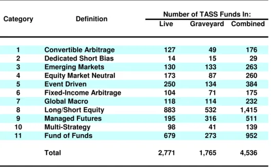
Table 6: Number of funds in the TASS Hedge Fund Live, Graveyard, and Combined databases, from February 1977 to August 2004.
The TASS database consists of monthly returns, assets under management and other fund-specific information for 4,781 individual funds from February 1977 to August 2004. The database is divided into two parts: “Live” and “Graveyard” funds. Hedge funds that
13
For further information about these data see http://www.hedgeindex.com (CSFB/Tremont indexes) and http://www.tassresearch.com (TASS). We also use data from Altvest, the University of Chicago’s Center for Research in Security Prices, and Yahoo!Finance.
are in the “Live” database are considered to be active as of August 31, 2004.14 As of August, 2004, the combined database of both live and dead hedge funds contained 4,781 funds with at least one monthly return observation. Out of these 4,781 funds, 2,920 funds are in the Live database and 1,861 in the Graveyard database. The earliest data available for a fund in either database is February 1977. TASS started tracking dead funds in 1994, hence it is only since 1994 that TASS transferred funds from the Live database to the Graveyard database. Funds that were dropped from the Live database prior to 1994 are not included
in the Graveyard database, which may yield a certain degree of survivorship bias.15
The majority of 4,781 funds reported returns net of management and incentive fees on a
monthly basis.16 and we eliminated 50 funds that reported only gross returns, leaving 4,731
funds in the “Combined” database (2,893 in the Live and 1,838 in the Graveyard database). We also eliminated funds that reported returns on quarterly—not monthly—basis, leav-ing 4,705 funds in the Combined database (2,884 in the Live and 1,821 in the Graveyard database). Finally, we dropped funds that did not report assets under management, or re-ported only partial assets under management, leaving a final sample of 4,536 hedge funds in the Combined database which consists of 2,771 funds in the Live database and 1,765 funds in the Graveyard database. For the empirical analysis in Section 4, we impose an additional filter in which we require funds to have at least five years of non-missing returns, leaving 1,226 funds in the Live database and 611 in the Graveyard database for a combined total of 1,837 funds. This obviously creates additional survivorship bias in the remaining sample of funds, but since the main objective is to estimate measures of illiquidity exposure and not
14
Once a hedge fund decides not to report its performance, is liquidated, is closed to new investment, restructured, or merged with other hedge funds, the fund is transferred into the “Graveyard” database. A hedge fund can only be listed in the “Graveyard” database after being listed in the “Live” database. Because the TASS database fully represents returns and asset information for live and dead funds, the effects of suvivorship bias are minimized. However, the database is subject to backfill bias—when a fund decides to be included in the database, TASS adds the fund to the “Live” database and includes all available prior performance of the fund. Hedge funds do not need to meet any specific requirements to be included in the TASS database. Due to reporting delays and time lags in contacting hedge funds, some Graveyard funds can be incorrectly listed in the Live database for a period of time. However, TASS has adopted a policy of transferring funds from the Live to the Graveyard database if they do not report over a 8- to 10-month period.
15
For studies attempting to quantify the degree and impact of survivorship bias, see Baquero, Horst, and Verbeek (2004), Brown, Goetzmann, Ibbotson, and Ross (1992), Brown, Goetzmann, and Ibbotson (1999), Brown, Goetzmann, and Park (1997), Carpenter and Lynch (1999), Fung and Hsieh (1997b, 2000), Horst, Nijman, and Verbeek (2001), Hendricks, Patel, and Zeckhauser (1997), and Schneeweis and Spurgin (1996).
16
TASS defines returns as the change in net asset value during the month (assuming the reinvestment of any distributions on the reinvestment date used by the fund) divided by the net asset value at the beginning of the month, net of management fees, incentive fees, and other fund expenses. Therefore, these reported returns should approximate the returns realized by investors. TASS also converts all foreign-currency denominated returns to U.S.-dollar returns using the appropriate exchange rates.
to make inferences about overall performance, this filter may not be as problematic.17 TASS also classifies funds into one of 11 different investment styles, listed in Table 6 and described in the Appendix, of which 10 correspond exactly to the CSFB/Tremont
sub-index definitions.18 Table 6 also reports the number of funds in each category for the Live,
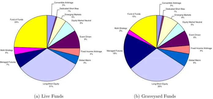
Graveyard, and Combined databases, and it is apparent from these figures that the rep-resentation of investment styles is not evenly distributed, but is concentrated among four categories: Long/Short Equity (1,415), Fund of Funds (952), Managed Futures (511), and Event Driven (384). Together, these four categories account for 71.9% of the funds in the Combined database. Figure 2 shows that the relative proportions of the Live and Graveyard databases are roughly comparable, with the exception of two categories: Funds of Funds (24% in the Live and 15% in the Graveyard database), and Managed Futures (7% in the Live and 18% in the Graveyard database). This reflects the current trend in the industry towards funds of funds, and the somewhat slower growth of managed futures funds.
Convertible Arbitrage 5% Dedicated Short Bias
1% Emerging Markets
5%
Equity Market Neutral 6%
Event Driven 9%
Fixed Income Arbitrage 4% Global Macro 4% Long/Short Equity 31% Managed Futures 7% Multi-Strategy 4% Fund of Funds 24%
(a) Live Funds
Convertible Arbitrage 3% Dedicated Short Bias
1% Emerging Markets
8%
Equity Market Neutral 5%
Event Driven 8%
Fixed Income Arbitrage 4% Global Macro 6% Long/Short Equity 30% Managed Futures 18% Multi-Strategy 2% Fund of Funds 15% (b) Graveyard Funds Figure 2: Breakdown of TASS Live and Graveyard funds by category.
3.1
CSFB/Tremont Indexes
Table 7 reports summary statistics for the monthly returns of the CSFB/Tremont indexes from January 1994 to August 2004. Also included for purposes of comparison are summary statistics for a number of aggregate measures of market conditions which we will use later
17
See the references in footnote 15.
18
This is no coincidence—TASS is owned by Tremont Capital Management, which created the CSFB/Tremont indexes in partnership with Credit Suisse First Boston.
as risk factors for constructing explicit risk models for hedge-fund returns in Section 6, and their definitions are given in Table 30.
Table 7 shows that there is considerable heterogeneity in the historical risk and return characteristics of the various categories of hedge-fund investment styles. For example, the
annualized mean return ranges from−0.69% for Dedicated Shortsellers to 13.85% for Global
Macro, and the annualized volatility ranges from 3.05% for Equity Market Neutral to 17.28%
for Emerging Markets. The correlations of the hedge-fund indexes with the S&P 500 are generally low, with the largest correlation at 57.2% for Long/Short Equity, and the lowest
correlation at−75.6% for Dedicated Shortsellers—as investors have discovered, hedge funds
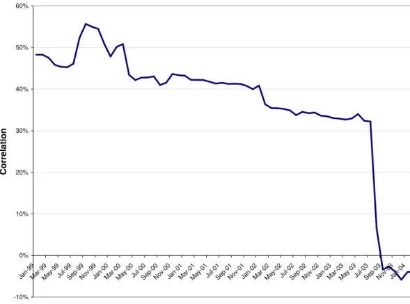
offer greater diversification benefits than many traditional asset classes. However, these correlations can vary over time. For example, consider a rolling 60-month correlation between the CSFB/Tremont Multi-Strategy Index and the S&P 500 from January 1999 to December 2003, plotted in Figure 3. At the start of the sample in January 1999, the correlation is
−13.4%, then drops to −21.7% a year later, and increases to 31.0% by December 2003 as
the outliers surrounding August 1998 drop out of the 60-month rolling window.
Although changes in rolling correlation estimates are also partly attributable to
estima-tion errors,19 in this case, an additional explanation for the positive trend in correlation
is the enormous inflow of capital into multi-strategy funds and fund-of-funds over the past five years. As assets under management increase, it becomes progressively more difficult for fund managers to implement strategies that are truly uncorrelated with broad-based market indexes like the S&P 500. Moreover, Figure 3 shows that the correlation between the Multi-Strategy Index return and the lagged S&P 500 return has also increased in the past year, indicating an increase in the illiquidity exposure of this investment style (see Getmansky, Lo, and Makarov, 2004 and Section 4 below). This is also consistent with large inflows of capital into the hedge-fund sector.
Despite their heterogeneity, several indexes do share a common characteristic: nega-tive skewness. Convertible Arbitrage, Emerging Markets, Event Driven, Distressed, Event-Driven Multi-Strategy, Risk Arbitrage, Fixed-Income Arbitrage, and Fund of Funds all have skewness coefficients less than zero, in some cases substantially so. This property is an indi-cation of tail risk exposure, as in the case of Capital Decimation Partners (see Section 1.1), and is consistent with the nature of the investment strategies employed by funds in those categories. For example, Fixed-Income Arbitrage strategies are known to generate fairly consistent profits, with occasional losses that may be extreme, hence a skewness coefficient
of −3.27 is not surprising. A more direct measure of tail risk or “fat tails” is kurtosis—the
19
Under the null hypothesis of no correlation, the approximate standard error of the correlation coefficient is 1/√60= 13%.
-30% -20% -10% 0% 10% 20% 30% 40% Ja n-99 Mar-9 9 May-9 9 Jul-9 9 Se p-99 Nov-9 9 Ja n-00 Mar-0 0 May-0 0 Jul-0 0 Se p-00 Nov-0 0 Ja n-01 Mar-0 1 May-0 1 Jul-0 1 Se p-01 Nov-0 1 Ja n-02 Mar-0 2 May-0 2 Jul-0 2 Se p-02 Nov-0 2 Ja n-03 Mar-0 3 May-0 3 Jul-0 3 Se p-03 Nov-0 3 Ja n-04 Date C or re la tio n Corr(R_t,SP500_t) Corr(R_t,SP500_t-1)
Figure 3: 60-month rolling correlations between CSFB/Tremont Multi-Strategy Index re-turns and the contemporaneous and lagged return of the S&P 500, from January 1999 to December 2003. Under the null hypothesis of no correlation, the approximate standard error
of the correlation coefficient is 1/√60 = 13% hence the differences between the
Variable Sample Size Mean Ann. SDAnn. Corr.
with S&P
500 Min Med Max Skew Kurt ρρρρ1 ρρρρ2 ρρρρ3
p-value of LB-Q CSFB/Tremont Indexes: Hedge Funds 128 10.51 8.25 45.9 -7.55 0.78 8.53 0.12 1.95 12.0 4.0 -0.5 54.8 Convert Arb 128 9.55 4.72 11.0 -4.68 1.09 3.57 -1.47 3.78 55.8 41.1 14.4 0.0 Dedicated Shortseller 128 -0.69 17.71 -75.6 -8.69 -0.39 22.71 0.90 2.16 9.2 -3.6 0.9 73.1 Emerging Markets 128 8.25 17.28 47.2 -23.03 1.17 16.42 -0.58 4.01 30.5 1.6 -1.4 0.7
Equity Market Neutral 128 10.01 3.05 39.6 -1.15 0.81 3.26 0.25 0.23 29.8 20.2 9.3 0.0
Event Driven 128 10.86 5.87 54.3 -11.77 1.01 3.68 -3.49 23.95 35.0 15.3 4.0 0.0
Distressed 128 12.73 6.79 53.5 -12.45 1.18 4.10 -2.79 17.02 29.3 13.4 2.0 0.3
Event-Driven Multi-Strategy 128 9.87 6.19 46.6 -11.52 0.90 4.66 -2.70 17.63 35.3 16.7 7.8 0.0
Risk Arb 128 7.78 4.39 44.7 -6.15 0.62 3.81 -1.27 6.14 27.3 -1.9 -9.7 1.2
Fixed Income Arb 128 6.69 3.86 -1.3 -6.96 0.77 2.02 -3.27 17.05 39.2 8.2 2.0 0.0
Global Macro 128 13.85 11.75 20.9 -11.55 1.19 10.60 0.00 2.26 5.5 4.0 8.8 65.0 Long/Short Equity 128 11.51 10.72 57.2 -11.43 0.78 13.01 0.26 3.61 16.9 6.0 -4.6 21.3 Managed Futures 128 6.48 12.21 -22.6 -9.35 0.18 9.95 0.07 0.49 5.8 -9.6 -0.7 64.5 Multi-Strategy 125 9.10 4.43 5.6 -4.76 0.83 3.61 -1.30 3.59 -0.9 7.6 18.0 17.2 SP500 120 11.90 15.84 100.0 -14.46 1.47 9.78 -0.61 0.30 -1.0 -2.2 7.3 86.4 Banks 128 21.19 13.03 55.8 -18.62 1.96 11.39 -1.16 5.91 26.8 6.5 5.4 1.6 LIBOR 128 -0.14 0.78 3.5 -0.94 -0.01 0.63 -0.61 4.11 50.3 32.9 27.3 0.0 USD 128 -0.52 7.51 7.3 -5.35 -0.11 5.58 0.00 0.08 7.2 -3.2 6.4 71.5 Oil 128 15.17 31.69 -1.6 -22.19 1.38 36.59 0.25 1.17 -8.1 -13.6 16.6 7.3 Gold 128 1.21 12.51 -7.2 -9.31 -0.17 16.85 0.98 3.07 -13.7 -17.4 8.0 6.2 Lehman Bond 128 6.64 4.11 0.8 -2.71 0.50 3.50 -0.04 0.05 24.6 -6.3 5.2 3.2
Large Minus Small Cap 128 -1.97 13.77 7.6 -20.82 0.02 12.82 -0.82 5.51 -13.5 4.7 6.1 36.6
Value Minus Growth 128 0.86 18.62 -48.9 -22.78 0.40 15.85 -0.44 3.01 8.6 10.2 0.4 50.3
Credit Spread (not ann.) 128 4.35 1.36 -30.6 2.68 3.98 8.23 0.82 -0.30 94.1 87.9 83.2 0.0
Term Spread (not ann.) 128 1.65 1.16 -11.6 -0.07 1.20 3.85 0.42 -1.25 97.2 94.0 91.3 0.0
VIX (not ann.) 128 0.03 3.98 -67.3 -12.90 0.03 19.48 0.72 4.81 -8.2 -17.5 -13.9 5.8
Table 7: Summary statistics for monthly CSFB/Tremont hedge-fund index returns and various hedge-fund risk factors, from January 1994 to August 2004 (except for Fund of Funds which begins in April 1994, and SP500 which ends in December 2003).
normal distribution has a kurtosis of 3.00, so values greater than this represent fatter tails than the normal. Not surprisingly, the two categories with the most negative skewness—
Event Driven (−3.49) and Fixed-Income Arbitrage (−3.27)—also have the largest kurtosis,
23.95 and 17.05, respectively.
Several indexes also exhibit a high degree of positive serial correlation, as measured
by the first three autocorrelation coefficients ρ1, ρ2, and ρ3, as well as the p-value of the
Ljung-Box Q-statistic, which measures the degree of statistical significance of the first three
autocorrelations.20 In comparison to the S&P 500, which has a first-order autocorrelation
coefficient of−1.0%, the autocorrelations of the hedge-fund indexes are very high, with values
of 55.8% for Convertible Arbitrage, 39.2% for Fixed-Income Arbitrage, and 35.0% for Event
Driven, all of which are significant at the 1% level according to the correspondingp-values.21
Serial correlation can be a symptom of illiquidity risk exposure, which is particularly relevant for systemic risk, and we shall focus on this issue in more detail in Section 4.
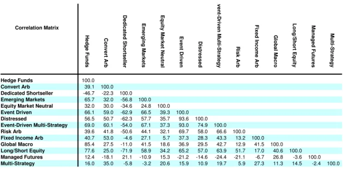
The correlations among the hedge-fund indexes are given in Table 8, and the entries also
display a great deal of heterogeneity, ranging from−71.9% (between Long/Short Equity and
Dedicated Shortsellers) and 93.6% (between Event Driven and Distressed). However, these
correlations can vary through time as Table 9 illustrates, both because of estimation error and through the dynamic nature of many hedge-fund investment strategies and the changes in fund flows among them. Over the sample period from January 1994 to December 2003, the correlation between the Convertible Arbitrage and Emerging Market Indexes is 31.8%, but during the first half of the sample this correlation is 48.2% and during the second half it is
−5.8%. A graph of the 60-month rolling correlation between these two indexes from January
1999 to December 2003 provides a clue as to the source of this nonstationarity: Figure 4
20
Ljung and Box (1978) propose the following statistic to measure the overall significance of the first k autocorrelation coefficients: Q = T(T+2) k X j=1 ˆ ρ2 j/(T−j) which is asymptoticallyχ2
k under the null hypothesis of no autocorrelation. By forming the sum of squared
autocorrelations, the statisticQreflects the absolute magnitudes of the ˆρj’s irrespective of their signs, hence
funds with large positive or negative autocorrelation coefficients will exhibit largeQ-statistics. See Kendall, Stuart and Ord (1983, Chapter 50.13) for further details.
21
The p-value of a statistic is defined as the smallest level of significance for which the null hypothesis can be rejected based on the statistic’s value. For example, a p-value of 73.1% for the Q-statistic of the Dedicated Shortseller index implies that the null hypothesis of no serial correlation can be rejected at the 73.1% significance level—at any smaller level of significance, say 5%, the null hypothesis cannot be rejected. Therefore, smallerp-values indicate stronger evidence against the null hypothesis, and largerp-values indicate stronger evidence in favor of the null. p-values are often reported instead of test statistics because they are easier to interpret (to interpret a test statistic, one must compare it to the critical values of the appropriate distribution; this comparison is performed in computing thep-value). See, for example, Bickel and Doksum (1977, Chapter 5.2.B) for further discussion of p-values and their interpretation.
H ed ge F un ds C on ve rt A rb D ed ic ate d S ho rts ell er E m er gin g M ar ke ts E qu ity M ar ke t N eu tra l E ve nt D riv en D is tre ss ed E ve nt -D riv en M ult i-S tra te gy R is k A rb Fix ed In co m e A rb G lo ba l M ac ro Lo ng /S ho rt E qu ity M an ag ed F ut ur es M ult i-S tra te gy Hedge Funds 100.0 Convert Arb 39.1 100.0 Dedicated Shortseller -46.7 -22.3 100.0 Emerging Markets 65.7 32.0 -56.8 100.0
Equity Market Neutral 32.0 30.0 -34.6 24.8 100.0
Event Driven 66.1 59.0 -62.9 66.5 39.3 100.0
Distressed 56.5 50.7 -62.3 57.7 35.7 93.6 100.0
Event-Driven Multi-Strategy 69.0 60.1 -54.0 67.1 37.3 93.0 74.9 100.0
Risk Arb 39.6 41.8 -50.6 44.1 32.1 69.7 58.0 66.6 100.0
Fixed Income Arb 40.7 53.0 -4.6 27.1 5.7 37.3 28.3 43.3 13.2 100.0
Global Macro 85.4 27.5 -11.0 41.5 18.6 36.9 29.5 42.7 12.9 41.5 100.0
Long/Short Equity 77.6 25.0 -71.9 58.9 34.2 65.2 57.0 63.9 51.7 17.0 40.6 100.0
Managed Futures 12.4 -18.1 21.1 -10.9 15.3 -21.2 -14.6 -24.4 -21.1 -6.7 26.8 -3.6 100.0
Multi-Strategy 16.0 35.0 -5.8 -3.2 20.6 15.9 10.9 19.7 5.9 27.3 11.3 14.5 -2.4 100.0
Correlation Matrix
Table 8: Correlation matrix for CSFB/Tremont hedge-fund index returns, in percent, based on monthly data from January 1994 to August 2004.
shows a sharp drop in the correlation during the month of September 2003. This is the first month for which the August 1998 data point—the start of the LTCM event—is not included in the 60-month rolling window. Table 10 shows that in August 1998, the returns for the
Convertible Arbitrage and Emerging Market Indexes were−4.64% and−23.03, respectively.
In fact, 10 out of the 13 style-category indexes yielded negative returns in August 1998, many of which were extreme outliers relative to the entire sample period, hence rolling windows containing this month can yield dramatically different correlations than those without it.
3.2
TASS Data
To develop a sense of the dynamics of the TASS database, in Table 11 we report annual frequency counts of the funds in the database at the start of each year, funds entering during the year, funds exiting during the year, and funds entering and exiting within the year. The table shows that despite the start date of February 1977, the database is relatively sparsely populated until the 1990’s, with the largest increase in new funds in 2001 and the largest number of funds exiting the database in the most recent year, 2003. The attrition rates reported in Table 11 are defined as the ratio of funds exiting in a given year to the number of existing funds at the start of the year. TASS began tracking fund exits starting only in 1994 hence attrition rates cannot be computed in prior years. For the unfiltered