Implications of return predictability for consumption dynamics and asset pricing

Carlo A. Favero Fulvio Ortu, Andrea Tamoni and Haoxi

Yang

Implications of return predictability for

consumption dynamics and asset pricing

Article (Accepted version)

(Refereed)

Original citation:

Favero, Carlo A. and Ortu, Fulvio and Tamoni, Andrea and Yang, Haoxi (2018) Implications of return predictability for consumption dynamics and asset pricing. SSRN Electronic Journal. ISSN 1556-5068

DOI: 10.2139/ssrn.2184254 © 2018 Elsevier

This version available at: http://eprints.lse.ac.uk/90426/

Available in LSE Research Online: October 2018

LSE has developed LSE Research Online so that users may access research output of the School. Copyright © and Moral Rights for the papers on this site are retained by the individual authors and/or other copyright owners. Users may download and/or print one copy of any article(s) in LSE Research Online to facilitate their private study or for non-commercial research. You may not engage in further distribution of the material or use it for any profit-making activities

or any commercial gain. You may freely distribute the URL (http://eprints.lse.ac.uk) of the LSE

Research Online website.

This document is the author’s final accepted version of the journal article. There may be differences between this version and the published version. You are advised to consult the publisher’s version if you wish to cite from it.

Implications of Return Predictability for

Consumption Dynamics and Asset Pricing

∗

Carlo A. Favero

Bocconi University & IGIER & CEPR

Fulvio Ortu

Bocconi University & IGIER

Andrea Tamoni

LSE

Haoxi Yang

Nankai University

This version: June 15, 2018

Abstract

Two broad classes of consumption dynamics - long-run risks and rare disasters - have proven successful in explaining the equity premium puzzle when used in conjunction with recursive pref-erences. We show that bounds a-l`a Gallant, Hansen and Tauchen (1990) that restrict the volatility of the Stochastic Discount Factor by conditioning on a set of return predictors constitute a useful tool to discriminate between these alternative dynamics. In particular we document that models that rely on rare disasters meet comfortably the bounds independently of the forecasting hori-zon and the asset classes used to construct the bounds. However, the specific nature of disasters is a relevant characteristic at the 1-year horizon: disasters that unfold over multiple years are more successful in meeting the predictors-based bounds than one-period disasters. Instead, over a longer, 5-year horizon, the sole presence of disasters - even if one-period and permanent - is sufficient for the model to satisfy the bounds. Finally, the bounds point to multiple volatility components in consumption as a promising dimension for long-run risks models.

J.E.L. CLASSIFICATION NUMBERS: G12, E21, E32, E44

Keywords: stochastic discount factor, predictors-based bounds, long run

∗_{We would like to thank two anonymous referees and the associate editor for their valuable comments. We also}

thank for helpful comments G. Bekaert, M. Chernov, D. Papanikolaou, N. Pavoni, C. Robotti, E. Sentana, and Yuzhao Zhang (FMA discussant), seminar participants at Manchester Business School, UBC, Hebrew University, Collegio Carlo Alberto, Warwick Business School, University of Piraeus, BI Norwegian Business School, HKUST Business School, REIM-SWUFE, and ICEF-HSE, and conference participants at the 2015 Asset Pricing Workshop (York), 20th Annual Conference of the Multinational Finance Society and FMA 2013 Annual Meeting.

†_{Deutsche Bank Chair in Quantitative Finance and Asset Pricing, Bocconi University, Department of Finance,}

Milan, 20136, Italy. e-mail: [email protected].

‡_{Bocconi University, Department of Finance, Milan, 20136, Italy. e-mail: [email protected].}

§_{London School of Economics, Department of Finance, London, WC2A 2AE, UK. e-mail: [email protected]} ¶_{Nankai Univeristy, School of Finance, Tianjin, 300350, China, e-mail: [email protected]}

1

Introduction

This paper shows that the Stochastic Discount Factor (SDF, henceforth) variation implied by return predictability is a useful moment to discriminate among leading asset pricing models that feature the same preference specification, but different consumption dynamics. This is important since multiple frameworks (notably long-run risks, rare disasters, and habit) have emerged as leading contenders to explain the equity premium puzzle (Mehra and Prescott, 1985), the volatility puzzle (Shiller, 1982), and other features of the aggregate stock market. The surge of several models that fit essentially the same aggregate moments begs the question as to which tools are suitable to disentangle the proposed asset pricing frameworks.

This paper exploits the predictability of asset returns to construct predictors-based variance bounds, i.e. bounds on the variance of those SDF that price a given set of returns conditional on the information contained in a vector of returns predictors. We focus our analysis on models based on recursive utility a-la Epstein and Zin (1989) and Weil (1990). This restricts our attention to two classes of models: long-run risks and rare disasters. While focusing on a single functional form for the SDF, our analysis investigates a wide range of specification for the state dynamics. We explore differences across frameworks - the emphasis in the long run risks model is on the first two conditional moments of consumption, while the rare disasters model puts emphasis on higher-order moments - and within the same framework - for example we look at multiperiod disasters with partial recovery against the case in which disasters are completely permanent. Using the requirement for the variance of the model-implied SDF to be larger than the variance dictated by the predictors-based variance bounds, we are able to discriminate between different specifications for the state variables. Formal statistical tests favor rare disasters over long run risks. The essential ingredient for the success of the rare disaster is the multi-period nature of disasters. The presence of recoveries after disasters is, instead, less important. Within the long-run risks framework, instead, our bounds favor a specification featuring multiple sources of stochastic volatility in the state dynamics.

We compute predictors-based bounds as in Gallant, Hansen, and Tauchen (1990) and Bekaert and Liu (2004). To make the bounds operational, we specify the set of asset returns to be

forecast, the predictors, and the forecasting horizons. We construct predictor based bounds for three alternative investment horizons - namely h = 1,4,20 quarters, and two alternative sets of returns: a first set that includes the equity market plus the returns from rolling a 3-month Treasury Bills over the horizon h, and a second set that adds the returns from equity value-growth portfolios to the first set. We employ as stock market predictors the dividend-price and consumption-wealth ratios, and as predictors of value strategies the portfolio’s book-to-market ratios. Despite selecting only predictors that are economically motivated by accounting identities (see Campbell and Shiller (1988) for the dividend-price ratio, Campbell and Mankiw (1989) and Lettau and Ludvigson (2001) for the consumption-wealth ratio, and Vuolteenaho (2002) for the book-to-market ratio), our bounds are sharp enough to discriminate the state dynamics across, and within, models. Also, looking at multiple horizons is important: whereas the intermediate 1−year horizon allows us to emphasize the importance of the multi-period nature of disasters versus the presence of recoveries, the long-horizon dilutes these differences.

Within the long-run risk framework we investigate both the Bansal, Kiku, and Yaron (2016) model, where the state variables are the first two conditional moments of log consumption growth, and the recent specification described in Schorfheide, Song, and Yaron (2018), in which the set of state variables is expanded to account for three separate volatility components: one governing the dynamics of the persistent cash flow growth component, and the other two controlling tempo-rally independent shocks to consumption and dividend volatility. Within the rare disasters class we concentrate on the framework of Nakamura, Steinsson, Barro, and Urs´ua (2013) since this specification allows for the possibility of recoveries after disasters, and the notion that disasters may unfold over several years, thus addressing recent critiques (see Constantinides and Ghosh, 2008; and Gourio, 2008a). Noteworthy, by suitably choosing the parameters space the Nakamura et al. (2013) model embeds the classical formulation of Rietz (1988) and Barro (2006) where disasters are permanent and occur in a single period.

Broadly speaking our work is related to the recent literature in asset pricing that looks at which of the many models that fit essentially the same aggregate moments is the “right”description of the underlying risk. Hansen and Scheinkman (2009) and Borovicka, Hansen, Hendricks, and

Scheinkman (2011) propose to compare structural models by computing the term structure of (model-implied) exposures of cash flows to shocks, as well as the compensation for these exposures. Zviadadze (2017) builds on their results, and propose to compare models using impulse response function (IRF) of expected returns to economic shocks. She concludes that volatility shocks are important for the long-run risks model to replicate the shape and level of expected equity returns impulse responses in the data. This result is consistent with our finding that multiple volatility components (like in Schorfheide et al. (2018)) are needed for a model to satisfy comfortably the restrictions on the variance of the SDF dictated by our predictors-based bounds at multiple horizons. Since both our predictors-based bounds and the IRFs proposed by Zviadadze (2017) rely on the predictability of asset returns, it is not surprising that we achieve similar conclusions. Importantly, whereas our bounds are model free, Zviadadze (2017) uses information from the model to identify the IRFs in the data. Entropy bounds provide another tool to discriminate across asset pricing models. For example, Backus, Chernov, and Zin (2014), Bakshi and Chabi-Yo (2012) and Ghosh, Julliard, and Taylor (2011) build on the recent information-theoretic literature to restrict the admissible regions for the SDF, and its permanent and transitory components. Interestingly, the one-period entropy restricts high-order cumulants of the log SDF. We instead restrict first and second moments of the (raw, not log) SDF. Also, whereas the multiperiod entropy exploits information from bond yields, we exploit information only from equity returns to discriminate across models.

Our work is related to Cochrane and Hansen (1992), who have been the first to look sys-tematically at Hansen and Jagannathan (1991) bounds across horizons to ascertain the relative performance of different asset pricing models. The present paper extends their analysis in several directions. First, we account explicitly for the effect of returns predictability at different horizons. Moreover, we highlight the interplay between preferences, dynamics and horizons in a wider vari-ety of models. From this standpoint, in particular, we extend the comparative horizons analysis of Cochrane and Hansen (1992) to models that explicitly contain a low frequency component, such as the long-run risk and rare disaster models, and investigate if and how different specifications of this components can make asset pricing puzzles less pronounced at longer horizons. Finally, we

account for estimation uncertainty in both the bounds and the model-implied SDFs.

Kirby (1998) provides an explicit link between linear predictability and the Hansen and Ja-gannathan (1991) bounds. Whereas Kirby (1998) investigates whether the ability of predictors to forecast a given set of return is correctly priced by some rational asset pricing model, in the sense that there exist SDFs that price correctly those dynamic strategies which condition on the predictors, our interest here is different: we want to exploit the informational content of a given

set of predictors to investigate the potential of a given asset pricing model to price a given set of

returns.

Kan and Robotti (2016) compare the long-run risks, the Campbell and Cochrane (1999) habit, and disaster risk models by means of unconditional SDF bounds as an empirical example to illustrate the importance of reporting confidence intervals for the Hansen and Jagannathan (1991) bounds instead of only presenting their point estimates. Their analysis is silent on the use of the bounds to discriminate alternative state dynamics for a fixed set of preferences (in particular Kan and Robotti (2016) do not investigate the Schorfheide et al. (2018) specification with multiple volatility components, nor they compare multiperiod disasters against one-period, permanent disaster models). Most importantly, the Kan and Robotti (2016) analysis is unconditional, and it is not informative about the role of predictability in asset returns, and thus about the role of the forecasting horizon, for constructing the bounds and separating models.

The rest of this paper is organized as follows. Sections 2 discusses the interplay between predictability, bounds and asset pricing models from the standpoint of the predictors-based vari-ance bounds. Section 3 documents the existence of significant predictable variation in aggregate stock market and value-growth equity portfolios, and shows how conditioning information plays an important role in the construction of the bounds at different horizons. We then assess whether various SDF specifications are consistent with the predictors-based bounds. Section 4 concludes. The online Appendix reports details on the estimation of the different asset pricing models and investigates the impact of misspecification of the conditional moments on our results.

2

Predictability, Variance Bounds, and Asset Pricing

In this section we briefly summarize the bounds implied by asset returns on the volatility of SDFs, in both their unconditional and conditional form. Assuming that conditioning is based on a set of return predictors, we show how to use the conditional variance bounds to assess two leading classes of asset pricing models, long run risks and rare disasters. For completeness, we briefly review the main characteristics of the consumption dynamics and the SDFs associated with these two classes of models.

2.1

Predictability of returns and variance bounds

Suppose that N assets are traded at a given time t, with returns vector Rt+h, where h is the

investment horizon. We denote by µ the vector of unconditional mean returns, and by Σ their unconditional covariance matrix. Recall that an SDF that prices the returns Rt+h is a random

variable mt+h that satisfies the pricing equation

E(mt+hRt+h) = 1 , (1)

where 1 is the unit vector. Letting then E(mt+h) = ν, in their seminal paper Hansen and

Jagannathan (1991), showed that the variance V ar(mt+h) of any SDF with mean ν satisfies the

following relationship:

V ar(mt+h)=(1−νµ) T

Σ−1(1−νµ)≡σ2_HJ(ν) , (2)

where the quadratic form in ν appearing at the right-hand-side takes the name of unconditional Hansen-Jagannathan bound, or HJ bound for short. To establish this fact Hansen and Jagan-nathan (1991) show that

is not only a legitimate SDF, but it is in fact the SDF with minimum variance among all the SDFs with mean ν.

Next, we consider the case in which a vectorZtpredicts the returnsRt+h, i.e.V ar(µt)>0 where

µt ≡E[Rt+h|Zt]. We concentrate our attention on the SDFs that price returns conditionally on

the realizations of the predictors Zt, that is

E(mt+hRt+h|Zt) =1 . (4)

Importantly, while the law of iterated expectations guarantees that any such SDF also prices the returns Rt+h unconditionally, in general an SDF that satisfies the unconditional pricing equation

fail to price correctly the returns when the information in the predictors Zt is accounted for.

Therefore, the set of SDFs that price returns conditionally on Zt is a subset of the set of SDFs

that satisfy the unconditional pricing equation.

We fix now an SDF mt+h that prices returns conditional on Zt, we let νt ≡ E[mt+h|Zt]

and ν = E(νt), and we characterize the SDF mZt+h with minimum variance among all the SDFs

that price returns conditionally and whose mean is ν. The solution to this problem is supplied by Gallant et al. (1990), who show that mZ

t+h is obtained by replacing in (3) the unconditional

moments with the conditional ones, i.e.

mZ_t+h =νt+ (1−νtµt) T

Σ−_t1(Rt+h−µt) (5)

where Σt is the conditional variance-covariance matrix.

The predictors-based boundσ2

Z(v) is then defined as the function that maps the mean of mZt+h

into its variance. In fact, to make this relationship more transparent, Bekaert and Liu (2004) work on the expression of V ar mZ_t+h to show that

σ2 Z(v)≡V ar mZt+h = Eh 1− ν−b 1−dµt T µtµTt + Σt −1 1− ν−b 1−dµt i −Eh 1− ν−b_1−dµt T µtµTt + Σt −1 µt i (6)

where b = E h µT_t µtµTt + Σt −1 1 i and d = E h µT_t µtµTt + Σt −1 µt i . Given v, therefore, σ2_Z(v) is a quadratic form in ν that yields the minimum variance across all SDFs that price the returns conditionally on the information in Zt and whose unconditional mean is v. It is readily seen that

the quadratic form σ2

Z(v) lies above σHJ2 (ν) for any value of v. As mentioned above, in fact,

the law of iterated expectation implies that any SDF which prices returns conditionally on Zt

does so unconditionally as well, hence E mZ t+hRt+h

=1. Since mHJ

t+h is the SDF with minimum

variance among all the SDFs with mean ν, it follows immediately that σ2

Z(v) ≡ V ar mZt+h ≥ V ar mHJ t+h ≡σ2

HJ (ν), an inequality that in fact holds strictly banning degenerate cases.

To illustrate the effect of predictability on the bounds we report in Panel A of Figure 1 the un-conditional bounds along with the un-conditional bounds based on two predictors, the dividend-price ratio and the consumption-wealth ratio. Interestingly the gap between the unconditional and con-ditional bounds increases with the holding period as a consequence of the fact that predictability increases with the horizon. In Section 3.3 we will exploit these bounds to compare alternative asset pricing models.

2.2

Predictors-based bounds, consumption dynamics and asset pricing

In a nutshell, a representative-agent asset pricing model is characterized by a couple Xt, mXt+h

where Xt ⊂ Ωt denotes the set of state variables of the model, Ωt the information set available

to the representative agent, and mX_t+h denotes the SDF of the model. Ideally, the state variables should represent a sufficient statistic of the information set Ωt, in the sense that the following

Euler condition should hold

E mX_t+hRt+h Ω_t =E mX_t+hRt+h X_t =1 . (7)

In words, if the state variables are a sufficient characterization of the information set Ωt then

the model SDF mX_t+h should price the returns from managed portfolios that condition on all the available information.

available to the optimizing agent. The law of iterated expectation applied to (7) imposes on any model-based SDF mX_t+h the necessary condition

E mX_t+hRt+h

Zt

=1 . (8)

Since the predictors-based bound σ_Z2(v) defined in equation (6) identifies a lower bound on the variance of any SDF that prices returns conditional on Zt, then any model-based SDF must satisfy

V ar mX_t+h≥σ2_Z(v). (9)

In the empirical part of the paper we use equation (9) to discriminate among leading asset pricing models. We focus on models where the representative consumer has preferences of the type developed by Epstein and Zin (1989) and Weil (1990). For this preference specification, Epstein and Zin (1989) show that the SDF takes the form

ln mX_t+h=A+B gt+h+C ra,t+h (10)

where ra,t+h denotes the (continuously compounded) return on an asset that delivers a dividend

equal to aggregate consumption, and A, B, C, are functions of the subjective discount factor, risk-aversion coefficient and intertemporal elasticity of substitution of the representative investor (see e.g. Bansal and Yaron (2004)).

In this paper we analyze models that, while having the same functional form for the SDF given in Eq. (10), encompass a variety of specifications for the state variables Xt generating the SDF.

The first model is the Bansal et al. (2016) model of long-run risks, where the consumption growth has the following dynamics:

gt+1 =µ+xt+σtηt+1 (11) xt+1 =ρxt+ϕeσtet+1 (12) σ2_t+1 =σ0+ν σ2t −σ 2 0 +σwwt+1

with the three shocks, η, e, and w being i.i.d Normal and uncorrelated. In this model the state variables are the first two conditional moments of log consumption growthgt, that isXt = (xt, σt2).

We also consider the specification of the long-run risks model described in Schorfheide et al. (2018). Whereas in Bansal et al. (2016) the time-varying volatility in realized and expected consumption growths is common, the Schorfheide et al. (2018) specification allows for two separate volatility components. Specifically, consumption evolves as follow:

gt+1 =µ+xt+σc,tηc,t+1 (13) xt+1 =ρxt+ p 1−ρ2_σ x,tet+1 (14) and

σi,t =ϕiσexp (hi,t), hi,t+1=ρhihi,t+σhi,twt+1 fori=c, x .

Therefore, in this model Xt = (xt, σc,t2 , σx,t2 ).

The last model is the Rare Disaster model of Nakamura et al. (2013). In this model the log consumption ct is the sum of three unobserved components:

ct=xt+zt+t (15)

where xt denotes “potential” consumption at time t; zt denotes the “disaster gap” – i.e., the

amount by which actual consumption differs from potential consumption due to current and past disasters, with t an i.i.d. normal shock. The occurrence of disasters is governed by a Markov

process It. It = 0 denotes “normal times” and It = 1 denotes times of disaster. Disasters affect

consumption in two ways. First, a disaster at time t generate a one-off permanent shift in the level of potential consumption, denoted by θt. Second, a disaster at time t causes a temporary

drop in consumption, denoted by φt. Specifically we have

∆xt = µ+ηt+Itθt (16)

where µ is the average growth rate of trend consumption and ηt is an i.i.d. normal shock to

the growth rate of trend consumption. We also study two restricted version of the Nakamura et al. (2013) model, a version of the model with “permanent disasters”and a version of the model with “permanent and one-period disasters”. Both cases require that φt =θt. On top of this, the

model with permanent and one-period disasters sets the probability of exiting a disaster to one. Finally, in this case the state variables Xts are (It, zt).

3

Empirical Results

Our empirical investigation is articulated in two steps. First, we review the predictability of raw returns within a standard, linear forecasting model (see Section 3.1). Given the evidence of significant predictability, we compute the predictors-based bound σ2

Z(ν) for different sets of assets

and horizons, and compare them with the unconditional bounds (see Section 3.2). Importantly, we establish that the predictors employed in our linear forecasting model are indeed useful in sharpening the diagnostic efficacy of variance bounds with respect to the unconditional case.

Second, we compare the variability of model-implied SDFs against the predictors-based bounds (see Section 3.3). We show that, by exploiting the first conditional moment of returns across horizons, the predictors-based bounds provide a useful model-selection tool that permits either to set models apart, or to select the common behavior among apparently different models.

3.1

The predictive model

To conduct our empirical analysis, we consider three horizons and two alternative sets of assets for each horizon. Specifically, we concentrate on horizons of h = 1,4,20 quarters, and for each horizon we consider alternatively the following two sets of returns:

1. SET A: the equity market returns plus the returns from rolling a three-month Treasury Bill over the holding period h;

2. SET B: the returns from SET A plus the returns on nine equity portfolios based on value strategies.

In particular the market return is the (gross) return on the value weighted portfolio of all stocks traded in the NYSE, the AMEX, and NASDAQ. With regard to value portfolios, we form quintiles and use the returns on the High, Medium, and Low portfolios. We measure value using three alternative signals, which gives us a total of nine portfolios. The first measure of value is standard, and it is based on the ratio of the book value to the market value of equity, as in Fama and French (1992). Following Asness and Frazzini (2013) we use the most recent market values to compute the ratios. Also consistent with previous literature, we exclude financial firms: a given book-to-market ratio might indicate distress for a non-financial firm, but not for a financial firm (see Fama and French, 1995). We denote this value signal BMi,t,Ex.f in.. Since many financial

firms are large and in the investment opportunity set of most investors, we also consider a second set of industry-adjusted book-to-market ratios: BMi,t,Ind.adj., which subtract from eachBMi,t the

value-weighted average book-to-market ratio of the industry to which stock ibelongs. Finally, we also perform a sort across 17 industries, using for each industry the average book-to-market ratio as value signal (denoted IndustryBMi,t). All returns are gross and deflated using the consumer

price index (CPI).

These two sets correspond to a universe of equity assets whose return properties are the subject of much scrutiny in the empirical asset pricing research. In particular SET A relates our findings to the classical unconditional HJ (1991) bounds, as well as to the vast literature that tackles the equity premium puzzle of Mehra and Prescott (1985). We expand SET A using value strategies for three reasons. First, the (unconditional) premium of value over growth portfolios is considered as one of the most prominent anomalies in the cross sectional asset pricing literature (see Cochrane, 2011). Second, the returns on value strategies should be informative about cash flows and discount rate news since short-duration assets like value stocks are more sensitive to cash flow shocks, whereas long-duration assets like growth stocks are more sensitive to discount rate shock (see e.g. Lettau and Wachter (2007)). Finally, and most important for our purpose, value strategies are predictable in the time series, as documented by Asness, Friedman, Krail, and Liew (2000), Cohen, Polk, and Vuolteenaho (2003), and Baba Yara, Boons, and Tamoni (2018).

classical value portfolio based on the BMHigh,t,Ex.f in. signal.

[Insert Table 2]

In contrast to the simple random walk view, stock returns do seem predictable, and markedly more so the longer the horizon. To review this claim we use a typical specification that regresses rates of return on lagged predictors. In particular we consider the following linear predictive system:

R_ti_+h =β₀i_,h+β₁i_,hZ_ti +ui_t+h (18) where i=M, V stands for Market and Value portfolios, respectively, andZt = ZtM, ZtV

denotes the vector of returns’ predictors, potentially different for the aggregate market and the value portfolios. As mentioned above, the holding period ranges from one quarter to five years, i.e. h = 1,4,20 quarters. The stock market return predictors are the dividend-price ratio, dpt, and

the consumption-wealth ratio, cayt, i.e.

Z_tM = [dpt, cayt] .

The value portfolio returns predictors are dpt, cayt,and the book-to-market ratio of the portfolio

i= 1, . . . ,9, generically denoted BMi,t, i.e.

Z_tV = [Z_tM, BMi,t] .

Finally, we forecast the real return on the T-bill using the lagged yield spread and the level of the US treasury-bill rates. This is consistent with the literature on term structure which uses principal components to forecast bond returns (see Duffee, 2013).

The choice ofdptas a stock market predictor is motivated by the present value logic, see

Camp-bell and Shiller (1988), while the choice of cayt follows from a linearization of the accumulation

equation for aggregate wealth in a representative agent economy, see Campbell and Mankiw (1989) and Lettau and Ludvigson (2001). Similarly, the book-to-market ratio BMi,t can be justified as

They are all “noisy” predictors of future asset returns. According to the present value model, the dividend yield should either forecast dividend growth or returns, or both. Empirically, the dividend yield does forecast excess returns and not dividend growth. Table 3-Panel A presents regressions of the real stock returns Rs

t+h ontoZtA. Although theR2 = 4.7% at quarterly horizon

is low, it then rises with the horizon, reaching a value of about 51%, at the 5 years horizon. Each variable has an important impact on forecasting long horizon returns: using the price-dividend ratio as the sole forecasting variable, for instance, would lead to an R2 _{of “only” 22% at the 5}

years horizon. Table 3-Panel B presents regressions of the real returns on the classical value port-folio onto Z_tV = [Z_tM, BMHigh,t,Ex.f in.], and it confirms the pattern of predictability observed for

market returns. Overall, these results are consistent with much of the recent empirical research on the predictability of aggregate stock returns (see Campbell (1987), Cochrane (2001; 2008), and Lewellen (2004) among others) and of value returns (see Asness et al. (2000), Cohen et al. (2003), Baba Yara et al. (2018)).

[Insert Table 3]

3.2

Predictors-based bounds across horizons

It seems apparent from Table 3 that expected returns vary over time. To evaluate by how much the predictors sharpen the diagnostic ability of the variance bounds, we compare the predictors-based bounds to the unconditional HJ bounds.

To compute the predictors-based bounds we use Eq. (6). In particular, we use the linear predictive model in equation (18) to obtain the first and second conditional moments of asset returns, µt and Σt. The conditional covariance matrix for returns is estimated as the variance

matrix of residuals in the forecasting regressions.

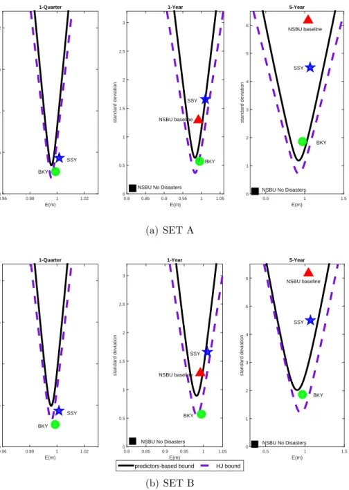
Figure 1(a) presents results for SET A for the investment horizonsh = 1,4,20 quarters. In each panel we report the efficient bounds generated with conditioning information (solid lines) along with the unconditional HJ bounds (dashed lines) that make no use of conditioning information. Similar to Cochrane and Hansen (1992), Figure 1(a) shows that the bottom of the mean standard deviation frontier shifts up and to the left as we increase the investment horizon. Importantly,

the picture shows that the predictability across horizons documented in Table 3 translates into a tighter lower bound on the variance of the SDF. In particular Figure 1(a) shows that the predictor-based bounds are sharper relative to the unconditional ones. For instance, the minimum point of the frontier at the 1-year (5-year) horizon obtained using conditioning information is about 1.98 (1.79, respectively) times sharper than the unconditional lower bound, thereby substantiating the incremental value of conditioning information in asset pricing applications. The difference between the bounds with and without conditioning information across horizons reflects the predictability documented in Table 3.

Figure 1(b) presents the same analysis for SET B. In this case, the use of conditioning infor-mation yields a bound that is about 1.47 (1.34) times the unconditional HJ bound at the 1-year (5-year, respectively) horizon. Upon comparing Figures 1(a) with 1(b), moreover, we observe that expanding the number of assets, i.e. moving from SET A to SET B, leads to a bound that is tighter than the one obtained using only returns from SET A.

[Insert Figures 1 about here]

Figures 1 imparts two conclusions. First, these figures highlight the three effects that are at work simultaneously: the conditioning information embedded in moments of returns, the horizon at which this information becomes relevant and the set of assets available for investment. The tightening of the volatility bounds is the combination of these three forces simultaneously at work. Second, although in the predictive regressions the role of the information contained in the predictors becomes more apparent as we lengthen the investment horizon, the predictors-based bounds reveal the important role played by conditioning information even at short horizons.

3.3

Predictors-based bounds and asset pricing models

Predictor-based bounds can be used to evaluate alternative specifications of the dynamics of the state variables under the same structure for preferences. In this paper we restrict our attention to models that rely on Epstein-Zin-Weil recursive preferences.

The models we investigate have been described in Section 2.2. We focus on estimated version of these models since we want to quantify the impact of parameter uncertainty on the mean

and volatility of their SDFs. Deep parameters of all three classes of models are estimated using a long span of the data to better capture the overall low frequency variations in asset prices and macroeconomic data and to reduce the measurement errors that arise from seasonalities and other measurement problems (see e.g. Wilcox, 1992). Finally, all models have been solved by well established methods that facilitate the computation of the first and second unconditional moments of their SDFs. Specifically, for the the rare disasters model, we solve numerically for a fixed point for the price of the consumption claim as a function of the state(s) of the economy. This method has been used by Campbell and Cochrane (1999), Nakamura et al. (2013), and Wachter (2013), among others. For the long-run risks models, we follow Bansal and Yaron (2004) and use a linearized solution method based on the Campbell and Shiller (1988) present-value relation.

The online Appendix B reports details on the estimation of the different asset pricing models considered in the paper. For the reader’s convenience, Tables B1, B2, and B3 in the online Appendix report, for each model, the complete specification of the parameter values for preferences and exogenous state dynamics, along with the standard errors of the estimated parameters.

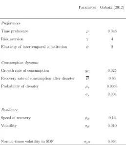
It is worth noting that a number of recent papers (see e.g. Gourio (2008b), Gabaix (2012), Wachter (2013)) propose versions of the rare disasters model that employ time-varying probability and/or severity of disasters to explain the predictability and volatility of stock returns, among other anomalous features of asset returns. Unfortunately the effect of estimation uncertainty on the moments of a model-implied SDF cannot be evaluated in any of these papers since they rely solely on calibration. Hence, we relegate to Section B.2.2 of the online Appendix an investigation of their performances.

Finally, it is important to stress that the models under consideration have all been estimated using information from the joint dynamics of consumption, dividends and aggregate equity market prices. Since all these models achieve a very good fit, it is not surprising that judging them using the very same cash flows and equity market moments used in the estimation step is not very informative. We show this fact in Table 1: all models feature low risk aversion, they all have low volatility of consumption, and yet they all deliver an (unconditional) equity risk premium comparable to the data. The main purpose of this paper is to show that the distance between

the model-implied SDF and the predictors-based bound is a statistics effective for discriminating across these models.

[Insert Table 1]

3.3.1 Model-implied SDFs and predictors-based bounds

To provide some intuition about the ability of the model-implied SDFs to satisfy the predictors-based bounds, first we abstract from parameter and small-sample uncertainty, and we use a single simulation run to infer the (population) mean and volatility of the SDF of each model. Specifically, we simulate 600,000 monthly observations (50,000 years) of the model-implied SDF for the long-run risks model, and 50,000 annual observations for the rare disaster model. We return to the issue of parameter and small-sample uncertainty in Section 3.3.3.

Figure 1 displays the predictors-based bounds and the SDFs generated by the different models for different horizons and for different sets of test assets. The predictors-based bound are displayed along with the classical HJ bound. For the long-run risks, we report with a circle the SDF for the Bansal et al. (2016) specification, and with a star the SDF for the Schorfheide et al. (2018). For the disasters model of Nakamura et al. (2013), the triangle and square correspond to the SDF in the baseline case and a “No Disaster” case, respectively. The “No Disasters” case features a long sample in which agents expect disasters to occur with their normal frequency but none actually occur. In all cases, the mean and the standard deviation of the SDFs reported in the figures represent population values obtained using estimated parameters.

A first observation that emerges clearly from Figures 1 concerns the importance of jointly considering conditioning information and horizons for the equity premium puzzle. Figure 1(a) shows that the SDFs of all models satisfy the unconditional HJ bounds at the 1-year horizon. This is essentially a graphical representation of the fit of these models, see Table 1. However, the conclusions are different when we incorporate conditioning information. In this case the classical long-run risks model with one time-varying volatility process struggles to meet the bounds, whereas the specification with multiple volatility components lies exactly on top of the predictors-based bound at the 1-year horizon, and satisfies the 5-year horizon bound comfortably. As expected,

using SET B (see Figure 1(b)), i.e. exploiting the additional predictable information from value strategies, exacerbates these results: the classical long-run risks models fall largely below the predictors-based bounds (while still marginally satisfying the 1- and 5-years unconditional bounds), whereas the Schorfheide et al. (2018) specification lies slightly outside of the predictors-based bound at the 1-year horizon, but it is still within the bounds at the 5-year horizon. The baseline specification of the disasters model makes it comfortably within the bounds at all relevant horizon, while the no-disaster case is always outside.

Importantly, had we considered the 1-year bounds with no conditioning information, we would have concluded that the equity premium puzzle, and to a lesser extent the unconditional value premium, could be resolved as long as sufficient time-nonseparability is incorporated in preferences. However, the predictors-based bounds highlight that what really matters is the interaction between preferences and the consumption dynamics.

The figures shed also some light on the long-horizon behavior of the SDFs from the competing models. This is interesting since frictions or measurement errors can disrupt the link between returns and consumption growth at high frequencies, while leaving the relation intact at low fre-quencies and long horizons. Hence, one would expect for asset pricing puzzles to be less pronounced at longer horizons (see e.g. Daniel and Marshall (1997)). With the visual aid of Figure 1 we can see that this expectation is fulfilled when no conditioning information is incorporated: the 5-year unconditional HJ bound is satisfied with good margin by all models, with the only exception of the no-disaster case. However, this changes significantly at the light of the predictors-based bound at the 5-year horizon. Focusing on SET B, we observe that the rare disasters model satisfies the predictor based bounds with a good margin, the long-run risk model with multiple volatility stands at the bounds, while the standard long-run risk model finds it onerous to satisfy the bounds at such a long horizon. Moreover, we show in Section 3.3.3 that accounting for statistical uncertainty sharpens the discrimination across models that we have highlighted so far.

The results in this section point to an interesting fact about the role played by preferences and state dynamics. Although the rare disasters and long-run risks models share the same preferences for early resolution of uncertainty, the two model-implied SDFs have very different behaviors.

This can be explained by the different ways the long-run risks and the rare disasters decompose consumption. Both models assume that the level of log consumption includes a deterministic trend and a stochastic trend. In the long-run risk model (see Eqs. (11) and (12), or (13) and (14) for the specification with two stochastic volatilities, one in realized and one in expected consumption growth), the growth rate of the stochastic trend captures expected consumption growth and contains (i) a persistent component, (ii) long-run variation in volatility. In the rare disaster model (see Eqs. (15) and (16)), on the other hand, the growth rate of the stochastic trend captures potential consumption and follows a jump process. Differently from the long-run risk, the rare disaster model of Nakamura et al. (2013) incorporates also a transitory component in the log consumption level - labeled disaster gap, see (17) - which allows for partial recoveries after disasters. Our predictors-based bounds favor a specification of the growth rate of the stochastic trend in consumption with jumps and recoveries compared with a specification with a persistent component and stochastic volatility. Within the long run risk models, instead, the predictors-based bounds favor a specification where the i.i.d. and persistent components of consumption growth feature separate stochastic volatilities.

3.3.2 The rare disaster model under the magnifying lens

A natural question is whether the superior performance of the Nakamura et al. (2013) model stems from the multiperiod nature of disasters (recall that the indicatorItin Eq. (16) may take the value

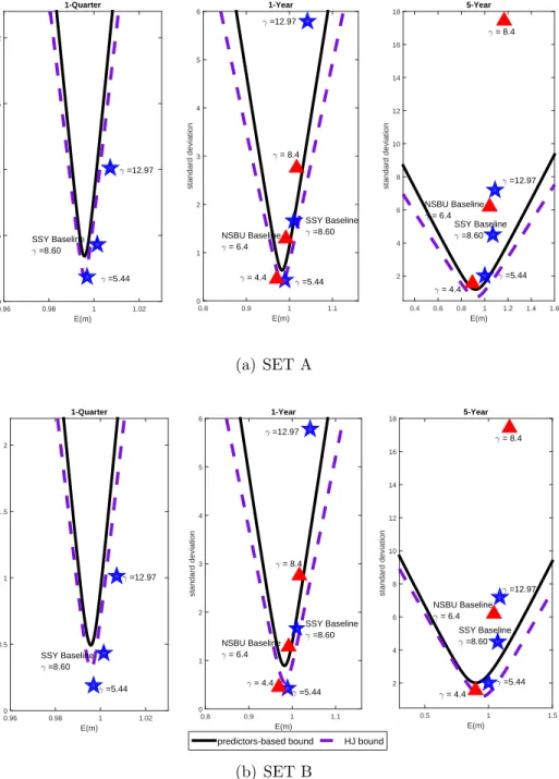
of 1 over multiple years), or from the partial recoveries after disasters, see Eq. (17), or from both. To address this point, in Figure 2 we consider two specifications of the Nakamura et al. (2013) rare disasters model in addition to the baseline economy analyzed so far. While all specifications have recursive preferences, they allow for different disaster dynamics. In particular we compare the model-implied SDF of Nakamura et al. (2013) (red triangle), with the SDF of a model in which disasters are completely permanent but unfold over several years (black triangle), and with the SDF of a model with permanent-and-one-period disasters of the type analyzed in Barro (2006) (blue triangle). Importantly, both the permanent, and permanent-and-one-period disasters model have been re-calibrated to deliver the same (observed) equity premium of 4.8%. Whereas the

baseline model matches the equity premium with a coefficient of relative risk aversion γ = 6.4, this value forγyields an equity premium of 10% when disasters are permanent, and an implausible 47% in the permanent-and-one-period disasters case. Thus, to match the equity premium in the data we setγ = 4.4 in the permanent disasters case, andγ = 3.0 in the permanent-and-one-period disasters case (see Table 1).

By comparing the baseline model with the permanent disasters model we can assess the im-portance of allowing for recoveries after disasters. In turn, by comparing the baseline model with the permanent-and-one-period disasters model we can assess the role of the multi-period nature of disasters. Looking at the one-year horizon, we observe that the SDF from the permanent model satisfies the predictors-based bounds (solid line), while it struggles when we incorporate returns on value strategies, whereas the SDF from the permanent-and-one-period disasters model is be-low the predictors-based bound independently from the test assets used. This fact highlights the important role played by the multi-period nature of disasters at the one-year horizons. Turning to the longer, five-years horizon, we observe that all specifications meet comfortably the predictors based bounds (the only exception is the permanent-and-one-period disasters model laying right on the bounds when SET B is considered). This fact highlights the importance of rare disasters for long-run dynamics independently from whether the disasters unfold over several years, or whether recoveries are allowed.

[Insert Figure 2 about here]

Putting together the evidence in Figures 1 and 2, we conclude that disaster dynamics are important to meet the predictorsbased bounds over the long run but the exact specification -e.g. whether disasters unfold over multiple years or whether they are systematically followed by recoveries - is less relevant. At shorter horizon, in order to meet the predictors-based bounds it is instead key to have multiperiod disasters, whereas partial recovery matters to a lesser extent.

The evidence so far points to the ability of the predictors-based bounds to discriminate across models. We next quantify the robustness of these conclusions when we account for estimation uncertainty.

3.3.3 How uncertain is the distance from the bounds?

In this section we evaluate whether the difference between the estimated model-implied variance of the SDF, V ar mX

t

, and the estimated predictors-based bound, σ2

Z(v), is large in a statistical

sense. To properly compare the moments of the model-implied SDF with the variance bounds we must account for two sources of uncertainty. First, the computation of the mean and variance of a model-implied SDF relies on the estimates of the exogenous state dynamics, and hence it reflects the uncertainty in the parameters describing these dynamics. Second, since the volatility bounds are estimated from the data, they must reflect the uncertainty surrounding the linear predictive model used to compute the conditional moments of returns, see Eq. (18). Hereafter, we account for these sources of uncertainty to obtain the finite sample distribution of the difference ∆ = V ar mX

t

−σ2

Z(v) (see Cecchetti, Lam, and Mark (1994) and Burnside (1994) for a related

approach). For the models under scrutiny we draw the parameters for the state dynamics using the values given in the online Appendix, see Tables B1, B2, and B3. We draw the coefficients of each asset return predictors analogously. Given these parameters, for each model we simulate an SDF of length equal to our dataset, i.e. 742 months. Finally, we compute the model-implied variance of the SDFs, the predictors-based bounds, and their difference. We repeat this exercise 10000 times.

The results are summarized in Table 4, for SET A and SET B. We start by looking at the rightmost block. The results reflect the estimation uncertainty in both the predictors-based bounds and the moments of the model-implied SDF. The first conclusion that emerges from Table 4 is that independently from the horizon and test assets considered, the SDF of the rare disaster model satisfies comfortably the predictors-based bound even after accounting for estimation uncertainty. Interestingly, within the long-run risks class, the novel specification of Schorfheide et al. (2018) with multiple volatility components constitutes a noticeable improvement upon the classical long-run risks model based on a single time-varying volatility. Indeed, the Schorfheide et al. (2018) model now satisfies the 1-year and 5-year predictor-based bounds constructed from SET A, although it still fails the bounds constructed from SET B.

The remaining two blocks of Table 4 report a decomposition of the uncertainty in the com-parison of V ar mX_t with σ2_Z(v). Following Cecchetti et al. (1994), we think of this uncertainty as arising from three basic sources. Given the expected value of the SDF, v, there is uncertainty in both the location of the bound, σ2

Z(v), and the standard deviation implied by the model,

V ar mX t

. In addition, there is uncertainty induced by the fact that the mean of the SDF for the model, v, must be estimated. The leftmost block reports the estimated distance for a fixed mean of the SDF. The middle block of the table reports the uncertainty in ∆ that arises solely from randomness in v. If no uncertainty in the mean of the SDF is considered then all models, except for the no-disasters model, meet the volatility restriction at the 1- and 5-year horizons, for both SET A and SET B, with a 5% confidence level (see leftmost panel). Thus, uncertainty surrounding the volatility bounds is sufficient to make the SDFs satisfy the restrictions if one is fully confident about the location of the mean of the SDF. However, once the uncertainty about the mean of the SDF is accounted for, the conclusions are reversed (see the middle block) and, when using SET B, all models fail to meet the volatility restrictions with the sole exception of the rare disaster model. As one would expect, re-introducing uncertainty about the bounds helps the model: moving from the middle to the rightmost block shows that ∆ gets closer to positive values. However, the uncertainty on the bounds is not large enough to undo the uncertainty in the mean of the SDF. Hence, by comparing the distance of a model-implied SDF across the different columns in Table 4, it is clear that the main source of uncertainty lies in the fact that v must be estimated.

In sum, this section shows that by incorporating conditioning information from a well-established set of stock predictors, the predictors-based bounds are a useful tool to assess the performance of asset pricing models at multiple horizons. It is worth noting that each asset pricing model parametrization approximates quite reasonably the (annual) unconditional equity premium and the real risk-free return, while simultaneously calibrating closely to the first two unconditional mo-ments of consumption growth (see Table 1). The rare disaster model handily meets the predictor-based bounds across horizons and asset classes, even after accounting for estimation uncertainty. The classical version of the long-run risks model with a single common source of stochastic

volatil-ity (see Bansal et al. (2016)) fails to meet the restrictions imposed by the predictor-based bounds at the 1-year horizon, with the standard deviation of their SDFs never approaching the bounds. The version of the long-run risks that accommodates multiple volatility components (see Schorfheide et al. (2018)) represents an improvement in the sense that it satisfies the 1-year bound con-structed from SET A. At long horizons, finally, while the classical long-run risks model with one time-varying volatility process generates an SDF not volatile enough independently from the test assets considered, the modified long-run risks model with multiple volatility components satisfies the predictors-based bound when using SET A but fails when we consider our largest set of equity returns.

3.4

Model-implied SDF, predictors-based bounds and sensitivity to

risk aversion

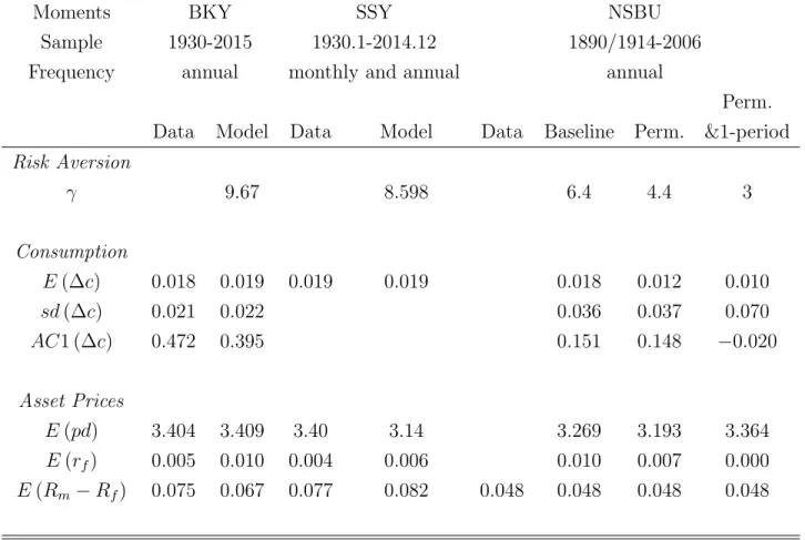
In this section, we inspect the sensitivity of model-implied SDFs to the coefficient of relative risk aversion (γ). To this end, we simulate and compare the model-implied SDFs with both high and low values of γ in addition to the baseline specification considered so far (see Figure 1).

Figure 3 displays the predictors-based bounds, and the SDFs generated by the Schorfheide et al. (2018) (stars) and the Nakamura et al. (2013) (triangles) models for different values of γ. For the Schorfheide et al. (2018) model, we simulate the model using the 5%, 50% and 95% posterior values of the estimated risk aversion reported in Table 5 of Schorfheide, Song, and Yaron (2016). Specifically, in the baseline specification γ equals 8.60, while it equals 5.44 and 12.97 for the low and high specifications, respectively. These values imply an equity premium of about 8.2% in the baseline case (see Table 1), and 4.24% and 13.36% for the low and high γ values. For the Nakamura et al. (2013) model, the baseline specification features a risk aversion of 6.4, which corresponds to an equity premium of 4.8% (see Table 1). We also analyze the case whenγ is set to 4.4 and 8.4. These low and high values imply an equity premium of 2% and 8.3%, respectively (see Table 7 in Nakamura et al. (2013)).

The figure shows that increasing risk aversion improves substantially the performance of the long-run risks model at the 1-year horizon, and that of the rare disasters model at the 5-year horizon. However, an important observation is in order.

Risk aversion is not a free parameter, and the higher levels of γ in the two models generate equity premia that are not in line with the data. In particular, setting γ = 8.4 in the Nakamura et al. (2013) model delivers an equity premium of 8.3%, which is higher than any of the estimates in Table 1. Similarly, a baseline level ofγ = 8.6 generates in the Schorfheide et al. (2018) model an equity premium of 8.2%. This evidence is even more important at the light of the recent literature documenting a decline in the equity premium (see e.g. Guvenen, 2003; Lettau, Ludvigson, and Wachter, 2007; and McGrattan and Prescott, 2005).

In sum, increasing risk aversion tends to deliver implausible results for the equity premium, and the dynamics of consumption become the key ingredient to fix the volatility of the SDF. This observation reinforces the usefulness of tools that discriminate between competing models of consumption dynamics and asset pricing. We believe that our predictors-based bounds give a positive contribution in this direction.

4

Conclusions

We have investigated the capability of asset pricing models that rely on recursive utility a-la Epstein and Zin (1989) and Weil (1990) to capture the Stochastic Discount Factor variation implied by return predictability. The models we picked fit essentially the same aggregate macro and asset-pricing moments, and thus a natural question arises as to which model provides the “right” description of the underlying sources of risks in the economy.

Our predictors-based bounds favor rare disasters dynamics over specifications which are based on long-run risks. Interestingly, the horizon over which we compute the bounds represents an important choice that conveys useful, discriminatory information. For instance, within the rare disaster class, the 1-year predictor-based bounds provide insights about the nature of disasters: a key ingredient for the model to fit the bounds is the presence of disasters that unfold over multiple years, whereas the role of recoveries after disasters is less relevant. Our bounds computed

over a longer 5-year horizon show instead that the sole presence of disasters - even if permanent and one-period - suffices to make the model-implied SDF able to meet the bounds. Within the long-run risks class, our predictors-based bounds point to a specification that features multiple volatility components as a promising avenue for future research. However, the predictability of value strategies, once incorporated into the bounds, represent a hurdle that even a long-run risks specification with multiple volatility components finds hard to overcome. Rare, multiperiod disasters prove instead successful even when confronted with bounds that embed information from value portfolios.

We conclude that our predictors-based bounds provide a fruitful new way of comparing different models to the data. A natural extension of our work would be to compare models featuring habits preferences, but featuring different dynamics such as Campbell and Cochrane (1999) and its variant proposed by Bekaert and Engstrom (2010).

SUPPLEMENTARY MATERIAL

Internet Appendix: The Internet Appendix contains a detailed description of the: (A) Data set used for the empirical analysis; (B) Estimation approach and parameter values for each asset pricing model; (C) Method to compute the difference between the estimated model-implied standard deviation of the SDF, σ mX_t , and the estimated predictors-based bound, σZ(v);

(D) Impact of mispecified conditional moments in constructing the predictors-based bounds.

References

Asness, C., and A. Frazzini. 2013. The Devil in HML’s Details. The Journal of Portfolio

Man-agement 39:49–68.

Asness, C., J. Friedman, R. J. Krail, and J. M. Liew. 2000. Style Timing: Value vs. Growth. The

Journal of Portfolio Management 26:50–60.

Baba Yara, F., M. Boons, and A. Tamoni. 2018. Value Timing: Risk and Return Across Asset Classes .

Backus, D., M. Chernov, and S. Zin. 2014. Sources of Entropy in Representative Agent Models.

Journal of Finance 69:51–99.

Bakshi, G., and F. Chabi-Yo. 2012. Variance bounds on the permanent and transitory components of stochastic discount factors. Journal of Financial Economics 105:191–208.

Bansal, R., D. Kiku, and A. Yaron. 2016. Risks for the long run: Estimation with time aggregation.

Journal of Monetary Economics 82:52 – 69.

Bansal, R., and A. Yaron. 2004. Risks for the Long Run: A Potential Resolution of Asset Pricing Puzzles. Journal of Finance 59:1481–1509.

Barro, R. J. 2006. Rare Disasters and Asset Markets in the Twentieth Century. Quarterly Journal

of Economics pp. 823–866.

Bekaert, G., and E. Engstrom. 2010. Asset Return Dynamics under Bad Environment Good Envi-ronment Fundamentals. NBER Working Papers 15222, National Bureau of Economic Research, Inc.

Bekaert, G., and J. Liu. 2004. Conditioning Information and Variance Bounds on Pricing Kernels.

Borovicka, J., L. P. Hansen, M. Hendricks, and J. A. Scheinkman. 2011. Risk-Price Dynamics.

Journal of Financial Econometrics 9:3–65.

Burnside, C. 1994. Hansen-Jagannathan Bounds as Classical Tests of Asset-Pricing Models.

Jour-nal of Business and Economic Statistics 12:pp. 57–79.

Campbell, J. Y. 1987. Stock returns and the term structure. Journal of Financial Economics

18:373 – 399.

Campbell, J. Y., and J. Cochrane. 1999. Force of Habit: A Consumption-Based Explanation of Aggregate Stock Market Behavior. Journal of Political Economy 107:205–251.

Campbell, J. Y., and N. G. Mankiw. 1989. Consumption, Income, and Interest Rates: Reinter-preting the Time Series Evidence. NBER Working Papers 2924, National Bureau of Economic Research, Inc. URL http://ideas.repec.org/p/nbr/nberwo/2924.html.

Campbell, J. Y., and R. J. Shiller. 1988. The Dividend-Price Ratio and Expectations of Future Dividends and Discount Factors. Review of Financial Studies 1:195–228.

Cecchetti, S., P.-s. Lam, and N. C. Mark. 1994. Testing Volatility Restrictions on Intertemporal Marginal Rates of Substitution Implied by Euler Equations and Asset Returns. Journal of

Finance 49:123–52.

Cochrane, J. H. 2001. Asset Pricing. Princeton University Press.

Cochrane, J. H. 2008. The Dog That Did Not Bark: A Defense of Return Predictability. Review

of Financial Studies 21:1533–1575.

Cochrane, J. H. 2011. Presidential address: Discount rates. The Journal of finance 66:1047–1108. Cochrane, J. H., and L. P. Hansen. 1992. Asset Pricing Explorations for Macroeconomics. NBER

Working Papers 4088, National Bureau of Economic Research, Inc.

Cohen, R. B., C. Polk, and T. Vuolteenaho. 2003. The Value Spread. The Journal of Finance

78:609–642.

Constantinides, G. M., and A. Ghosh. 2008. Asset Pricing Tests with Long Run Risks in Con-sumption Growth. NBER Working Papers 14543, National Bureau of Economic Research, Inc. Daniel, K., and D. Marshall. 1997. Equity-premium and risk-free-rate puzzles at long horizons.

Macroeconomic Dynamics 1:452–484.

Duffee, G. 2013. Forecasting interest rates. In Handbook of economic forecasting, vol. 2, pp. 385–426. Elsevier.

Epstein, L. G., and S. E. Zin. 1989. Substitution, Risk Aversion, and the Temporal Behavior of Consumption and Asset Returns: A Theoretical Framework. Econometrica 57:937–69.

Fama, E. F., and K. R. French. 1992. The Cross-Section of Expected Stock Returns. The Journal

of Finance 47:427–465.

Fama, E. F., and K. R. French. 1995. Size and book-to-market factors in earnings and returns.

The Journal of Finance 50:131–155.

Gabaix, X. 2012. Variable rare disasters: An exactly solved framework for ten puzzles in macro-finance. The Quarterly Journal of Economics 127:645–700.

Gallant, A. R., L. P. Hansen, and G. Tauchen. 1990. Using conditional moments of asset payoffs to infer the volatility of intertemporal marginal rates of substitution. Journal of Econometrics

45:141–179.

Ghosh, A., C. Julliard, and A. P. Taylor. 2011. What is the Consumption-CAPM missing? An informative-Theoretic Framework for the Analysis of Asset Pricing Models. Fmg discussion papers, Financial Markets Group.

Gourio, F. 2008a. Disasters and recoveries. The American Economic Review 98:68–73.

Gourio, F. 2008b. Time-series predictability in the disaster model. Finance Research Letters

5:191–203.

Guvenen, F. 2003. A parsimonious macroeconomic model for asset pricing: habit formation or cross-sectional heterogeneity? RCER Working Papers 499, University of Rochester - Center for Economic Research (RCER).

Hansen, L. P., and R. Jagannathan. 1991. Implications of Security Market Data for Models of Dynamic Economies. Journal of Political Economy 99:225–62.

Hansen, L. P., and J. A. Scheinkman. 2009. Long-term Risk: An Operator Approach. Econometrica

77:177–234.

Kan, R., and C. Robotti. 2016. The exact distribution of the Hansen–Jagannathan bound.

Man-agement Science 62:1915–1943.

Kirby, C. 1998. The restrictions on predictability implied by rational asset pricing models. Review

of Financial Studies 11:343–382.

Lazarus, E., D. J. Lewis, J. H. Stock, and M. W. Watson. 2016. HAR Inference: Kernel Choice, Size Distortions, and Power Losses. Tech. rep., NBER Discussion Papers.

Lettau, M., and S. Ludvigson. 2001. Consumption, Aggregate Wealth, and Expected Stock Re-turns. Journal of Finance 56:815–849.

Lettau, M., S. C. Ludvigson, and J. A. Wachter. 2007. The declining equity premium: What role does macroeconomic risk play? The Review of Financial Studies 21:1653–1687.

Lettau, M., and J. A. Wachter. 2007. Why is long-horizon equity less risky? a duration-based explanation of the value premium. The Journal of Finance 62:55–92.

Lewellen, J. 2004. Predicting returns with financial ratios. Journal of Financial Economics

74:209–235.

McGrattan, E. R., and E. C. Prescott. 2005. Taxes, Regulations, and the Value of US and UK Corporations. The Review of Economic Studies 72:767–796.

Mehra, R., and E. C. Prescott. 1985. The equity premium: A puzzle. Journal of monetary

Economics 15:145–161.

Nakamura, E., J. Steinsson, R. Barro, and J. Urs´ua. 2013. Crises and recoveries in an empirical model of consumption disasters. American Economic Journal: Macroeconomics 5:35–74. Rietz, T. A. 1988. The equity risk premium a solution. Journal of monetary Economics 22:117–

131.

Schorfheide, F., D. Song, and A. Yaron. 2016. Identifying long-run risks: A bayesian mixed-frequency approach. Tech. rep., National Bureau of Economic Research.

Schorfheide, F., D. Song, and A. Yaron. 2018. Identifying long-run risks: A bayesian mixed-frequency approach. Econometrica 86:617–654.

Shiller, R. J. 1982. Do Stock Prices Move Too Much to be Justified by Subsequent Changes in Dividends? American Economic Review 71:421436.

Vuolteenaho, T. 2002. What Drives Firm-Level Stock Returns? The Journal of Finance 57:233– 264.

Wachter, J. A. 2013. Can Time-Varying Risk of Rare Disasters Explain Aggregate Stock Market Volatility? The Journal of Finance 68:987–1035.

Weil, P. 1990. Nonexpected utility in macroeconomics. The Quarterly Journal of Economics

105:29–42.

Wilcox, D. W. 1992. The construction of US consumption data: some facts and their implications for empirical work. The American economic review pp. 922–941.

E(m) 0.96 0.98 1 1.02 standard deviation 0 0.5 1 1.5 2 1-Quarter E(m) 0.8 0.85 0.9 0.95 1 1.05 standard deviation 0 0.5 1 1.5 2 2.5 3 1-Year E(m) 0.5 1 1.5 standard deviation 0 1 2 3 4 5 6 5-Year SSY NSBU baseline BKY BKY SSY SSY NSBU baseline BKY

NSBU No Disasters _{NSBU No Disasters}

(a) SET A E(m) 0.96 0.98 1 1.02 standard deviation 0 0.5 1 1.5 2 1-Quarter E(m) 0.8 0.85 0.9 0.95 1 1.05 standard deviation 0 0.5 1 1.5 2 2.5 3 1-Year E(m) 0.5 1 1.5 standard deviation 0 1 2 3 4 5 6 5-Year

predictors-based bound HJ bound

SSY BKY SSY NSBU baseline BKY BKY SSY NSBU baseline

NSBU No Disasters NSBU No Disasters

(b) SET B

Figure 1 Predictors-based bound (σz(v)), Hansen-Jagannathan (1991) bound (σHJ(v)),

and model-implied SDFs – SET A and SET B. The figure displays the Hansen-Jagannathan (1991) bounds (dashed violet line) and the predictors-based bounds (solid black line). We follow Bekaert and Liu (2004) to construct the predictors-based bounds. To construct the bounds we use data from 1952Q2 to 2012Q3. The green circle and blue star correspond to the (average mean and standard deviation of the) SDF obtained from 10 simulation runs of 600,000 months of the Bansal et al. (2016) (BKY model) and Schorfheide et al. (2018) (SSY model) long-run risks models, respectively. The red triangle corresponds to the SDF obtained from 10 simulation runs of 50,000 years of the (baseline case of) Nakamura et al. (2013) rare disasters model. The black square corresponds to the no disasters case, i.e. it refers to a long sample in which agents expect disasters to occur with their normal frequency but none actually occur.

E(m) 0.95 0.96 0.97 0.98 0.99 1 1.01 1.02 standard deviation 0.2 0.4 0.6 0.8 1 1.2 1.4 1.6 1.8 2 1-Year E(m) 0.6 0.7 0.8 0.9 1 1.1 1.2 standard deviation 0 1 2 3 4 5 6 5-Year Baseline Permanent Permanent and one period Permanent Baseline Permanent and one period (a) SET A E(m) 0.95 0.96 0.97 0.98 0.99 1 1.01 1.02 standard deviation 0.2 0.4 0.6 0.8 1 1.2 1.4 1.6 1.8 2 1-Year E(m) 0.6 0.7 0.8 0.9 1 1.1 1.2 standard deviation 0 1 2 3 4 5 6 5-Year

predictors-based bound HJ bound

Permanent and one period Permanent Baseline Permanent Permanent and one period Baseline (b) SET B

Figure 2 Rare disaster model-implied SDFs, Hansen-Jagannathan (1991) bound (σHJ(v)), predictors-based bounds (σz(v)) – SET A and SET B. The figure displays the

Hansen-Jagannathan (1991) bounds (dashed violet line) and the predictors-based bounds (solid black line). We follow Bekaert and Liu (2004) to construct the predictors-based bounds. To construct the bounds we use data from 1952Q2 to 2012Q3. The red triangle corresponds to the (average mean and standard deviation of the) SDF obtained from 10 simulations run of 50,000 years of the baseline Nakamura et al. (2013) case, in which the risk aversion parameter (γ) equals to 6.4 and IES equals to 2. The blue triangle corresponds to the SDF obtained from simulations of the permanent and one-period disasters case, in which γ is set to 3.0 and the IES to 2. The black triangle corresponds to the SDF obtained from simulations of the permanent but multiple disasters case, in which γ is set to 4.4 and the IES to 2.

E(m) 0.96 0.98 1 1.02 standard deviation 0 0.5 1 1.5 2 1-Quarter E(m) 0.8 0.9 1 1.1 standard deviation 0 1 2 3 4 5 6 1-Year E(m) 0.4 0.6 0.8 1 1.2 1.4 1.6 standard deviation 2 4 6 8 10 12 14 16 18 5-Year γ = 8.4 γ =5.44 SSY Baseline γ =8.60 γ = 4.4 SSY Baseline γ =8.60 γ =12.97 γ = 8.4 γ =12.97 SSY Baseline γ =8.60 NSBU Baseline γ = 6.4 γ = 4.4 γ =5.44 γ =12.97 NSBU Baseline γ = 6.4 γ =5.44 (a) SET A E(m) 0.96 0.98 1 1.02 standard deviation 0 0.5 1 1.5 2 1-Quarter E(m) 0.8 0.9 1 1.1 standard deviation 0 1 2 3 4 5 6 1-Year E(m) 0.5 1 1.5 standard deviation 2 4 6 8 10 12 14 16 18 5-Year

predictors-based bound HJ bound

γ =12.97 SSY Baseline γ =8.60 γ =5.44 γ =12.97 γ = 8.4 SSY Baseline γ =8.60 NSBU Baseline γ = 6.4 γ = 4.4 γ =5.44 γ =12.97 γ = 8.4 NSBU Baseline γ = 6.4 SSY Baseline γ =8.60 γ = 4.4 γ =5.44 (b) SET B

Figure 3 Model-implied SDFs, predictors-based bounds and sensitivity to risk aversion (γ) – SET A and SET B. The figure displays the Hansen-Jagannathan (1991) bounds (dashed violet line) and the predictors-based bounds (solid black line). We follow Bekaert and Liu (2004) to construct the predictors-based bounds. To construct the bounds we use data from 1952Q2 to 2012Q3. The blue stars correspond to the (average mean and standard deviation of the) SDF obtained from 10 simulations run of 600,000 months of the Schorfheide et al. (2018) model, with γ sets to 5.44, 8.60 (Baseline) and 12.97, respectively. The red triangles correspond to the (average mean and standard deviation of the) SDF obtained from 10 simulations run of 600,000 months of the Nakamura et al. (2013) model, with γ sets to 4.4, 6.4 (Baseline) and 8.4, respectively.

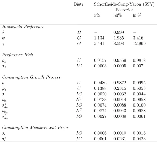
Table 1 Moments of consumption and asset returns. We report the data and model-implied (annualized) moments of consumption and asset returns for the three asset pricing models analyzed in the main text. For Bansal et al. (2016) (BKY), we take the values from their paper directly. For Schorfheide et al. (2018) (SSY), we take values from their working paper Schorfheide et al. (2016). For Nakamura et al. (2013) (NSBU), the model-implied moments of consumption growth and price-dividend ratios are computed by the authors. We simulate the model using the posterior mean of estimated values of parameters. ∆cis the annual consumption growth rate. pd is the the log of the end of year price over the twelve month trailing sum of dividends. rf is the

logarithm of the annual risk-free rate. (Rm−Rf) is the annual equity risk premium.

Moments BKY SSY NSBU

Sample 1930-2015 1930.1-2014.12 1890/1914-2006

Frequency annual monthly and annual annual

Perm. Data Model Data Model Data Baseline Perm. &1-period

Risk Aversion γ 9.67 8.598 6.4 4.4 3 Consumption E(∆c) 0.018 0.019 0.019 0.019 0.018 0.012 0.010 sd(∆c) 0.021 0.022 0.036 0.037 0.070 AC1 (∆c) 0.472 0.395 0.151 0.148 −0.020 Asset Prices E(pd) 3.404 3.409 3.40 3.14 3.269 3.193 3.364 E(rf) 0.005 0.010 0.004 0.006 0.010 0.007 0.000 E(Rm−Rf) 0.075 0.067 0.077 0.082 0.048 0.048 0.048 0.048

Table 2 Statistics of the Data. This table reports sample statistics of quarterly annualized nominal stock market and classical value portfolio returns. Stock market returns are nominal returns on the stock total returns on the value weighted portfolio of all stocks traded in the NYSE, the AMEX, and NASDAQ from CRSP. Classical value portfolio returns are nominal returns on the stock portfolio formed by the BMi,t,Ex.f in. ratio. Sample: 1952Q2−2012Q3.

Asset

Market Value Portfolio Mean return (% p.a.) 11.45 13.17 Standard deviation (% p.a.) 16.68 16.55

Table 3 Predictability of stock and portfolio returns. Panel A reports quarterly overlapping regressions of multiple horizon real gross stock market returns onto a constant, cayt, and the log

dividend-price ratio dpt. Panel B reports quarterly overlapping regressions of multiple horizon

real gross return on a classical value portfolio onto a constant, cayt,dpt, and the portfolio’s

book-to-market ratio BMHigh,t . The table reports coefficient estimates, the R2 of the regression, and,

Newey-West t-statistics in parentheses. Following Lazarus et al. (2016), we set the Newey-West truncation parameter toST =

3 2B

T, whereB = 8. We evaluate the test statistic using critical values from the tB. Critical values of Student’st-distribution with 8 degrees of freedom are 1.860,

2.306 and 3.355 at 10%, 5% and 1% significant level, respectively. Sample: 1952Q2: 2012Q3.

Panel A: Predictive regressions for stock market returns

Horizon (quarters) cayt

(t−stat) dpt (t−stat) R2(%) 1 0.84 (2.11) 0(3..0308) 4.7 4 3.19 (2.61) 0(3..1230) 17.0 20 16.06 (4.14) 0(4..6071) 51.2

Panel B: Predictive regressions for value portfolio returns

Horizon BMt (t−stat) cayt (t−stat) dpt (t−stat) R2_(%) 1 0.09 (3.18) (10..4851) −(−01..15)03 6.3 4 0.27 (3.21) (11..6449) −(−00..56)04 19.5 20 0.71 (3.07) (26..1254) (10..2335) 52.7