Testing Asymmetric-Information Asset Pricing Models
∗ Bryan KellyNew York University Alexander Ljungqvist New York University and CEPR
August 10, 2009
Abstract
Theoretical asset pricing models routinely assume that investors have heterogeneous informa-tion. We provide direct evidence of the importance of information asymmetry for asset prices and investor demands using plausibly exogenous variation in the supply of information caused by the closure of 43 brokerage firms’ research operations in the U.S. Consistent with predictions derived from a Grossman and Stiglitz-type model, share prices and uninformed investors’ demands fall as information asymmetry increases. Cross-sectional tests support the comparative statics: Prices and uninformed demand experience larger declines, the more investors are uninformed, the larger and more variable is stock turnover, the more uncertain is the asset’s payoff, and the noisier is the better-informed investors’ signal. We show that at least part of the fall in prices is due to expected returns becoming more sensitive to liquidity risk. Our results imply that information asymmetry has a substantial effect on asset prices and that a primary channel linking asymmetry to prices is liquidity.
∗We thank Anat Admati, Yakov Amihud, Brad Barber, Xavier Gabaix, Charles Jones, Marcin Kacperczyk, Ambrus
Kecsk´es, and Bryan Routledge (our WFA discussant) as well as audiences at Columbia, Berkeley, and the 2009 WFA meeting for helpful suggestions. Address for correspondence: Stern School of Business, New York University, 44 West Fourth Street, New York NY 10012-1126. Kelly: Phone 212-998-0368; e-mail [email protected]. Ljungqvist: Phone 212-998-0304; fax 212-995-4220; e-mail [email protected].
Theoretical asset pricing models routinely assume that investors have heterogeneous information. The goal of this paper is to establish the empirical relevance of this assumption for equilibrium asset prices and investor demands. To do so, we exploit a novel identification strategy which allows us to infer changes in the distribution of information among investors and hence to quantify the effect of information asymmetry on prices and demands. Our results suggest that information asymmetry has a substantial effect on prices and demands and that it affects assets through a liquidity channel.
Asymmetric-information asset pricing models typically rely on noisy rational expectations equilib-ria in which prices reveal the better-informed investors’ information only partially due to randomness in the supply of the risky asset. Random supply might reflect the presence of ‘noise traders’ whose demands are independent of information. Prominent examples of such models include Grossman and Stiglitz (1980), Hellwig (1980), Admati (1985), Wang (1993), and Easley and O’Hara (2004).
To derive empirical predictions representative of these models, Section I adapts the Grossman and Stiglitz model to show that an increase in information asymmetry leads to a fall in share price and a reduction in uninformed investors’ demand for the risky asset. Simple expressions for equilibrium prices reveal that an important channel linking information asymmetry and price is liquidity risk: Price falls because greater information asymmetry exposes uninformed investors to more liquidity risk. The model’s comparative statics relate the changes in price and demand to the fraction of investors who are better informed, the supply of the asset, uncertainty about the asset’s payoff, and the noisiness of the better-informed investors’ signal.
Testing a model of asset pricing with asymmetric information poses a tricky identification chal-lenge. Imagine regressing the change in investor demand on the change in a proxy for information asymmetry, such as the stock’s bid-ask spread. Interpreting the coefficient would be hard if, as is likely, there are omitted variables (such as changes in the riskiness of the company’s cash flows) which simultaneously affect bid-ask spreads and demand. Another problem is reverse causality. Spreads may increase precisely because demand is expected to fall. To overcome such simultaneity problems, we need a source of exogenous variation in the degree of information asymmetry in the asset market.
The Grossman and Stiglitz model and its descendants suggest what we should be looking for: An exogenous change in the cost of information about an asset’s future payoffs. These models demonstrate how an increase in information cost will increase information asymmetry by inducing fewer investors to purchase information. Exogeneity means, in this setting, that the change in information cost must affect prices and demands only via its effect on the asymmetry of information. The cost change would have to be independent of all other underlying determinants of asset prices and demands, particularly the asset’s future payoffs.
Equity research analysts are among the most influential information producers in financial mar-kets. We argue that their presence or absence affects the extent of information asymmetry.1 Suppose investors are heterogeneous in their information costs. All those whose costs exceed the price at which an analyst sells his research will purchase it. If the analyst were to stop selling research, investors would have to fall back on alternative information sources, and for some, the cost of becoming in-formed would exceed the benefit. (For instance, hedge funds or mutual funds likely have relatively low-cost substitute information sources, but retail investors presumably do not.) Thus, information asymmetry would increase following an analyst’s departure.
Consider the extreme case of a market in which each stock is covered by exactly one analyst. The ideal experiment would be to randomly ban analysts from researching some stocks. Because the cost of information substitutes for buyers of analyst research must (weakly) exceed the analyst’s asking price, the average cost of information would increase for the stocks that randomly lose research, and information asymmetry would increase as a result. An econometrician could then measure the effect of information asymmetry on equilibrium asset prices and investor demands.
Our empirical approach is to identify a quasi-experiment of this nature. We exploit reductions in the number of analysts covering a stock that resulted from 43 brokerage firms in the U.S. closing 1A large literature provides evidence that analyst research is an important channel through which information is impounded in stock prices; see, among others, Womack (1996), Barber et al. (2001), Gleason and Lee (2003), Jegadeesh et al. (2004), and Kelly and Ljungqvist (2008). Some scholars take the opposite view, regarding analysts mainly as cheerleaders for companies who produce biased research in the hope of currying favor with executives (see, for instance, James and Karceski (2006)). While ultimately an empirical question, the skeptics’ viewpoint should bias us against finding a relation between the presence of analysts and equilibrium prices and demands.
down their research departments between Q1, 2000 and Q1, 2008. For identification purposes, we view brokerage closures as a source of exogenous variation in the extent of analyst coverage and examine changes in prices and investor demands for affected stocks around the closure announcements.
Our identification strategy makes two assumptions. First, the coverage terminations must cor-relate with an increase in information asymmetry. This will be the case if information costs are heterogeneous, as we have argued. Second, they must affect price and demand only through their effect on information asymmetry. In particular, they must be uninformative about the affected stocks’ future prospects. Unless a brokerage firm closed down its research department because its analysts had foreknowledge of imminent falls in some companies’ share prices (which seems unlikely), broker-age closures are plausibly exogenous. We discuss in Section II the reasons why so many brokerbroker-age firms have quit research since 2000. We also show empirically that our sample terminations are un-informative about the future prospects of the affected companies while correlating with increases in information asymmetry, as required for identification.2
Our sample of coverage terminations is quite different from those previously studied in the analyst literature. McNichols and O’Brien (1997) and Scherbina (2008) argue that analysts usually termi-nate coverage to avoid having to issue a sell recommendation when they expect future performance declines. Reasons to avoid issuing a sell include not wanting to upset an investment banking client or jeopardize access to the company’s management in future. Unlike our closure-related terminations, such selective or endogenous terminations would not allow us to causally link price changes around coverage terminations to changes in information asymmetry.
The list of brokerage firms that exited equity research over our sample period includes both large firms (e.g., Wells Fargo) and smaller outfits (e.g., Schwab’s Soundview Capital Markets division) and encompasses both retail-oriented firms (e.g., First Montauk) and institutional brokerage houses (e.g., Emerald Research) and brokers with either generalist (e.g., ABN Amro) or specialist coverage (e.g., 2Our identification strategy is similar in spirit to Hong and Kacperczyk’s (2007). Like us, these authors exploit exogenous variation in coverage (in their case, variation due to mergers among brokerage firms with overlapping coverage universes), though their focus is on the effect of competition on the extent of bias in analyst forecasts.
Conning & Co.). In total, the 43 closures are associated with 4,429 coverage terminations. The closures were well publicized in the media and affected clients were notified directly. Other investors would learn which stocks were affected by a closure, and why, from so called termination notices or through various financial websites, such as Dow Jones’ marketwatch.com.
We test the model’s predictions in Section III. As predicted, both price and uninformed demand fall following a coverage termination. Cumulative abnormal returns average between −45 and −112 basis points on the day of an exogenous coverage termination, depending on the benchmark, and there is no evidence of reversal even one month later. Institutional investors—which are more likely to be better informed—increase their holdings of affected stocks by around 1.4% while retail investors— who are more likely to be uninformed—sell. We confirm these findings using an alternative and independent source of exogenous variation in analyst coverage, due not to brokerage closures but to the terrorist attacks of September 11, 2001.
Our cross-sectional tests support the comparative statics. Prices and, to a noisier extent, unin-formed demand experience larger declines, the more investors are uninunin-formed, the larger and more variable is turnover, the more uncertain is the asset’s payoff, and the noisier is the signal.
Finally, using the Acharya-Pedersen (2005) model of expected returns, we show that affected stocks become more exposed to liquidity risk following exogenous coverage terminations and, as a result, expected returns increase. We interpret this finding as support for the notion that prices fall on announcement of a brokerage closure in anticipation of greater information asymmetry which in turn increases uninformed investors’ liquidity-risk exposure and therefore their required returns.
Our tests contribute to our understanding of asset pricing by providing direct evidence of the role of asymmetric information, the channel through which it operates, and the magnitude of its effects on prices and demands. While the fact that our findings support the key mechanism of asymmetric-information asset pricing models is perhaps not unexpected, such direct evidence is in fact quite rare, due to the identification problems we noted earlier. Thus, our second contribution is to provide a clean identification strategy with which to capture exogenous changes in asymmetric information. The
extant literature has instead relied on a variety of proxies for information asymmetry, employed either in the cross-section or as within-firm changes. Both are potentially problematic: In the cross-section due to omitted variables and in differences because changes are unlikely to be exogenous.
Arguably the most notable proxy for information asymmetry in the empirical literature is Easley and O’Hara’s (1992)PIN measure. PIN is based on the idea that the presence of privately informed traders can be noisily inferred from order flow imbalances. Easley et al. (1996) show that PIN
correlates with measures of liquidity such as bid-ask spreads, while Easley, Hvidkjær, and O’Hara (2002) find that PIN affects expected returns. While we offer no opinion on the matter, PIN has proven controversial. Mohanram and Rajgopal (2006), for example, find that PIN is not priced if one extends Easley et al.’s (2002) sample period. Similarly, Duarte and Young (2008) show that
PIN is only priced to the extent that it proxies for illiquidity rather than information asymmetry. The advantage of our approach relative to this literature is that it exploits exogenous variation in the supply of information, thus side-stepping the need for a proxy for information asymmetry whose potential correlations with unobserved variables are unknown and contentious.
The bulk of the literature has bypassed the question of asymmetric information by instead focusing on the role of liquidity in asset pricing—perhaps because liquidity is considerably easier to measure than information asymmetry. Relevant empirical studies include Pastor and Stambaugh (2003), Amihud and Mendelson (1986), Amihud (2002), Hasbrouck and Seppi (2001), Bekaert, Harvey, and Lundblad (2007), Jones (2002), and Eleswarapu (1997). Following theoretical models such as Amihud and Mendelson (1986), Acharya and Pedersen (2005), and Huang (2003), these studies treat liquidity as exogenous. Our findings suggest that liquidity varies with information asymmetry, consistent with microstructure models such as Kyle (1985) and Glosten and Milgrom (1985). Thus, one fundamental driver of asset prices appears to be information asymmetry, consistent with the models of Grossman and Stiglitz (1980), Hellwig (1980), Admati (1985), Wang (1993), and Easley and O’Hara (2004).
Our paper is also loosely related to the analyst literature. While we are interested in coverage terminations purely as a source of exogenous variation with which to identify changes in the supply
of information, there is an active literature focusing on the causes and consequences of selective (as opposed to exogenous) terminations; see Khorana, Mola, and Rau (2007), Scherbina (2008), Kecskes and Womack (2009), Ellul and Panayides (2009), and Madureira and Underwood (2008).
I.
The Model
The setup follows Grossman and Stiglitz (1980). There is a unit mass of investors who have identical initial wealth,W0, and are risk-averse with CARA utility of consumption−e−C.3 Investors trade in
period 1 and consume in period 2. There is a risk-free asset with gross return R and a single risky asset with aggregate supply X ∼N( ¯X, σ2x) and payoff u= θ+η. Investors know θ and can engage in research at cost c >0 which results in a noisy signal sabout the risky asset’s payoff innovation, η∼N(0, σ2
u): s=η+v, withv∼N(0, σ2v).When investoriobserves the signal, his information set,
Fi, includes both sand the equilibrium price,P, though price information is then redundant. When sis not observed,P contains useful conditioning information for payoffu. As we will show later, the assumptions of a single risky asset and a single signal are not restrictive.
In addition to the investors, there may or may not be an analyst, working for a brokerage firm, who can also produce signal s. For simplicity, we assume the analyst disseminates s (in the form of earnings forecasts, research reports, or trading recommendations) for free. This mirrors institutional practice: Investors are not charged for each analyst report they receive, so at the margin, the cost of observing the analyst’s signal is zero. Brokers recoup the cost of producing research through account fees, trading commissions, or cross-subsidies from market-making or investment banking.4
In the analyst’s presence,sis public information, so information is symmetric. In his absence, we are in the Grossman-Stiglitz (1980) world where investors must decide whether to produce the signal privately. Grossman and Stiglitz show that in equilibrium, some fraction 0< δ <1 of the investors pay to acquire the signal. Thus, in the analyst’s absence, information is asymmetric.
3The risk aversion coefficient is assumed equal to unity for simplicity and without loss of generality.
4We leave the brokerage firm’s incentive to disclose the analyst’s signal unmodeled. For models that endogenize this decision, see Admati and Pfleiderer (1986), Fishman and Hagerty (1995), or Veldkamp (2006a).
Investors do not observe aggregate supply X. The three random variables of the model (X, η, and v) are assumed to be independent.
A. Equilibrium Effects
To determine the equilibrium effects of a coverage termination, we compare prices and demands for the risky asset in the symmetric information case, which results from an analyst’s presence, to the asymmetric information case that occurs in the analyst’s absence. The following proposition summarizes the equilibrium changes when the analyst ceases to produce research on the asset.
Proposition 1: Following a coverage termination, a strictly positive fraction 1−δof investors choose not to produce the signal themselves and so become uninformed, while a measure δ >0 of investors become privately informed. The price of the risky asset falls by
∆EP ≡E[Pasymm−Psymm] = − σ4uσ4vX σ¯ 2x (1−δ) R (σ2 u+σ2v) σ2 xσ4v+σ2vδ σ2uσx2+σ2uδ2+σ2vδ2 <0 (1)
as uninformed investors sell. Privately informed investors increase their demand for the risky asset by the amount ∆EID= (1−δ)σ 2 uσ2vX σ¯ 2x σ2 xσ4v+σ2vδ σ2uσx2 +σ2uδ2+σ2vδ2 >0. (2)
Proof: See Appendix A.
B. Discussion
CARA utility combined with Gaussian random variables implies that investors optimize their demands by trading off mean and variance conditional on their information set. (For details, see Appendix A.) A coverage termination affects only the information set of investors who decide not to produce the signal themselves. From their perspective, a coverage termination increases the conditional payoff variance while having a mean zero effect on their expected payoff. This lowers uninformed demand and thus equilibrium price. At a lower price, privately informed investors, whose payoff beliefs are
unchanged, are induced to increase their demand until the market-clearing condition is satisfied. Why does payoff uncertainty increase from the perspective of the uninformed? In the analyst’s absence, the uninformed do not observe s and so base their demand solely on the observed price, P. However, P is not fully revealing, because investors do not observe aggregate supply, X. As a result, the uninformed cannot simply back out the informed investors’ signal from observed prices; they cannot tell whether a price change reflects a change in aggregate supply or a change in the signal. Instead, they noisily infer the signal by forming an expectation of payoff u conditional on observed priceP. Thus, a coverage termination exposes the uninformed to aggregate supply risk.
More formally, Appendix A shows that, under rational expectations, both the symmetric and asymmetric-information equilibrium prices are linear in the signal and in aggregate supply:
Psymm = θ R + σ2u R(σ2 u+σ2v) s−σ 2 u R (1− σ2u σ2 u+σ2v )X (3) Pasymm=c1+c2s+c3X (4)
wherec2 >0 andc3<0 (the precise expressions can be found in Appendix A). Following Brennan and
Subrahmanyam (1996) and Amihud (2002), we can interpretXas trade volume and the coefficient on Xas the price impact of trade. Note that trades have a price impact even if information is symmetric, as long as the payoff is uncertain. This follows from risk aversion.
As the following corollary shows, the effect of a coverage termination is to increase the price impact of trade:
Corollary 1: Let the price impact of trade be defined as ∂P/∂X. Then the change in price impact of trade following a coverage termination is given by the quantity
∆(∂P/∂X) = c3+ σ2 u R(1− σ2 u σ2 u+σ2v ) (5) = −1 R σ2v σ2u δ+ σ2 v σ2x σ2 x σ4v+ δ2+δ σ2 u σ2x σ2 v+ σ2uδ2 + σ2u1− σ 2 u σ2 u+ σ2v ! <0.
Corollary 1 says that price falls as information asymmetry increases because price becomes more sensitive to aggregate-supply or liquidity risk. Thus, we have:
Corollary 2: Following a coverage termination, the asset’s expected return increases as the asset’s exposure to liquidity risk increases.
C. Robustness
In common with Grossman and Stiglitz (1980), our model makes two simplifying assumptions: There is a single risky asset, and there is a single signal s which, in our setting, can be produced by both the analyst and investors. Neither assumption is restrictive.
Easley and O’Hara (2004) extend the Grossman-Stiglitz model to multiple assets and show that information risk cannot be diversified away even in large portfolios. Intuitively, the uninformed are at an informational disadvantage for every asset in their portfolio and so information risk is priced in equilibrium in the way we have modeled it.
Multiple independent signals also do not change the conclusions. Suppose there are N analysts publishing public signals and M other signals that may be purchased at cost cj >0. An analyst’s
departure corresponds to a (weakly) positive shift in the cost schedule for the menu of possible signal combinations. In equilibrium, investors consume all the free signals and a Grossman-Stiglitz solution determines consumption of the costly signals. Any signal combination an investor consumed before the analyst’s departure is more expensive now, so fewer signals are consumed and the fraction of informed investorsδ falls. In the new equilibrium, prices drop due to the decrease in the supply of information and the accompanying increase in overall payoff uncertainty following a coverage termination.
Finally, we note that it is straightforward to recast the analysis within the Kyle (1985) setup. This would leave Proposition 1, the corollaries, and the comparative statics discussed in the next section qualitatively unchanged. What we call the change in the price impact of trade in Corollary 1 would be analogous to the change in Kyle’s λ. We prefer the Grossman and Stiglitz (1980) setting because a coverage termination effectively increases the cost of information, which in their model is
explicitly linked to the fraction of informed investors and thus to equilibrium prices and demand. In Kyle, on the other hand, the distribution of information is taken as exogenous.
D. Testable Implications
To guide our empirical analysis, we derive the following comparative statics.
The more investors become privately informed following a coverage termination, the fewer investors are affected by the loss of analyst information. Thus, we have:
Implication 1: The larger the fraction of privately informed investors among the company’s share-holders, the smaller is the negative price impact of a coverage termination and the smaller is the resulting increase in informed demand for the company’s stock:
∂∆EP ∂δ = 2δ(1−δ) + σ2v σx2σ4u σ4v X σ¯ 2x σ2 x σ4v+ σ2vδ2+ σv2δ σ2u σ2x+ σ2uδ2 2 R >0 ∂∆EID ∂δ = −σ2v σ2u X σ¯ x2 σ2x σ4v+ σv2 σ2u σ2x+δ( σ2v+ σ2u)(2−δ) σ2 x σ4v+ σ2vδ2+ σv2δ σ2u σ2x+ σ2uδ2 2 <0.
Corollary 1 states that a coverage termination increases the (negative) sensitivity of price to aggregate supply because the uninformed have a harder time filtering the signal from the price. Thus, stocks with larger aggregate supply experience larger price and demand changes:
Implication 2: The greater is mean aggregate supply, the larger is the negative price impact of a coverage termination and the greater is the resulting increase in informed demand for the stock:
∂∆EP ∂X¯ = −σ2x σ4v σ4u(1−δ) ( σ2 u+ σ2v)R σ2 x σ4v+ δ2+δ σ2 u σ2x σ2 v+ σ2uδ2 <0 ∂∆EID ∂X¯ = (1−δ) σ2u σ2v σ2x σ2 x σ4v+ σ2vδ2+ σv2δ σu2 σ2x+ σ2uδ2 >0.
inference problem is harder the more variable are the aggregate supply and payoff, which in turn increases the value of analyst research to the uninformed. Thus, we have the following implications:
Implication 3a: The more variable is aggregate supply, the larger is the negative price impact of a coverage termination and the greater is the resulting increase in informed demand for the stock:
∂∆EP ∂σ2 x = −σ 4 u σ4v X δ¯ 2(1−δ) σ2 x σ4v+ σ2vδ2+ σv2δ σ2u σ2x+ σ2uδ2 2 R <0 ∂∆EID ∂σ2 x = (1−δ) σ 2 u σ2v X δ¯ 2 σ2u+ σ2v σ2 x σ4v+ σ2vδ2+ σv2δ σ2u σ2x+ σ2uδ2 2 >0.
Implication 3b: The more variable is the asset’s payoff, the larger is the negative price impact of a coverage termination and the greater is the resulting increase in informed demand for the stock:
∂∆EP ∂σ2 u = −σ 2 u σ6v X σ¯ 2x (1−δ) σ2v σ2u σ2x+ 2 σ2uδ2+ 2 σ2x σ4v+ 2 σ2vδ2+ σ2vδ σ2u σ2x R ( σ2 u+ σ2v)2 σ2 x σ4v+ σ2vδ2+ σv2δ σ2u σ2x+ σ2uδ2 2 <0 ∂∆EID ∂σ2 u = (1−δ) σ 4 v X σ¯ 2x σ2v σ2x+δ2 σ2 x σ4v+ σ2vδ2+ σv2δ σ2u σ2x+ σ2uδ2 2 >0.
The effect of signal noise is more complicated. Consider the two extreme cases. If the signal is very precise, the uninformed can filter the signal from the observed price very effectively, so losing the signal has a negligible impact on demand and prices. If the signal is so noisy as to be essentially uninformative, the informed have little informational advantage over the uninformed. As a result, a coverage termination results in negligible information asymmetry among investors and so has little impact on demand and prices. In between these two extremes, losing a noisy but informative analyst signal increases the uninformed investors’ inference problem and so leads to a price fall and a decrease in uninformed demand. Thus, we have:
while its effect on the change in expected informed demand is hump-shaped: ∂∆EP ∂σ2 v = −σ 4 u σ2v X σ¯ 2x (1−δ) 2 σ2 u σ2vδ2+ σ2vδ σ4u σ2x+ 2 σ4uδ2− σ2x σ6v R ( σ2 u+ σ2v)2 σ2 x σ4v+ σ2vδ2+ σv2δ σ2u σ2x+ σ2uδ2 2 < 0 iff 2 σ 2 u σ2vδ2+ σ2vδ σ4u σ2x+ 2 σ4uδ2 σ2 x σ6v >1 ∂∆EID ∂σ2 v = (1−δ) σ 2 u X σ¯ 2x σ2 uδ2− σ2x σ4v σ2 x σ4v+ σ2vδ2+ σv2δ σ2u σ2x+ σ2uδ2 2 > 0 iff σ 2 uδ2 σ2 xσ4v >1.
II.
Identification and Sample
A. Identification Strategy
Our identification strategy is straightforward. To examine the effects of an increase in information asymmetry on prices and demands, we need a source of exogenous variation in information asymmetry. Rather than relying on observed changes in various proxies for information asymmetry—which may vary for endogenous reasons—we identify an exogenous shock to the information production about a stock. Specifically, we focus on terminations of analyst coverage that are the result of brokerage firms closing down their research departments. Identification requires that coverage terminations correlate with an increase in information asymmetry but do not otherwise correlate with price or demand.
As McNichols and O’Brien (1997) observe, coverage changes are usually endogenous. Coverage terminations, in particular, are often viewed as implicit sell recommendations (Scherbina (2008)). The resulting share price fall may hence reflect the revelation of an analyst’s negative view of a firm’s prospects rather than the effects of reduced research coverage. Similarly, an analyst may drop a stock because institutions have lost interest in it (Xu (2006)). If institutional interest correlates with price,
price may fall following a termination for reasons unrelated to changes in information asymmetry. We avoid these biases by focusing on closures of research operations, rather than selective ter-minations of individual stocks’ coverage. The last decade has seen substantial exit from research in the wake of adverse changes to the economics of producing research.5 The fundamental challenge for equity research is a public goods problem: Because research cannot be kept private, clients are reluctant to pay for it, and hence it is provided for free. In the words of one observer, “Equity research is a commodity and it is difficult for firms to remain profitable because research is a cost center.”6
Traditionally, brokerage firms have subsidized research with revenue from trading (“soft dollar commissions”), market-making, and investment banking. Each of these revenue streams has dimin-ished since the early 2000s. The prolonged decline in trading volumes that accompanied the bear market of 2000-2003 along with increased competition for order flow has reduced trading commis-sions and income from market-making activities. Soft dollar commiscommis-sions have come under attack both from the S.E.C.7 and institutional clients.8 Finally, concerns that analysts publish biased re-search to please investment banking clients (Michaely and Womack (1999), Dugar and Nathan (1995), Lin and McNichols (1998)) have led to new regulations, such as the 2003 Global Settlement, which have made it harder for brokerage firms to use investment banking revenue to cross-subsidize research. Brokerage firms have responded to these adverse changes by downsizing or closing their research operations. We ignore those that downsized (because it is hard to convincingly show the absence of selection bias in firing decisions) and focus on a comprehensive set of 43 closures that were announced between 2000 and the first quarter of 2008.9 These include investment banks such as Wells Fargo
Securities, retail brokerage firms such as Charles Schwab and First Montauk, institutional brokerage houses such as Emerald Research, and foreign banks such as ABN Amro and ING.
5See, for example, “Following Wells Fargo, Others May Exit Equities Trading”, Dow Jones, 3 August 2005. 6David Easthope, analyst with Celent, a strategy consultancy focused on financial services, quoted in Papini (2005). 7The SEC issued new interpretative guidance of the safe-harbor rule under Section 28(e) of the 1934 Securities Exchange Act, which governs soft dollar commissions, in 2006. See http://www.sec.gov/rules/interp/2006/34-54165.pdf. 8According to the TABB Group, a consultancy, nearly 90% of all larger institutional investors stopped or decreased use of soft dollars between 2004 and 2005 (BusinessWire, June 1, 2005).
9Our sample excludes Bear Stearns and Lehman Brothers, both of which failed in 2008 and were integrated into J.P. Morgan and Barclays Capital, respectively. Lehman in particular is not a suitable shock for identification purposes, because Barclays, which had no U.S. equities business of its own, took over Lehman’s entire U.S. research department.
B. Sample
The 43 brokerage closures are associated with 4,429 coverage terminations, after filtering out securities with CRSP share codes> 12 (including REITs, ADRs, non-common stocks, and closed-end funds), companies without share price data in CRSP, and 51 companies due to be delisted within the next 60 days. We identify the affected stocks using the coverage table of Reuters Estimates, which lists, for each stock, the dates during which each broker and analyst in the Reuters database actively cover a stock; the I/B/E/S stop file, which has similar (albeit less reliably dated) information; and the termination notices which were sent to brokerage clients and can be retrieved from Investext.
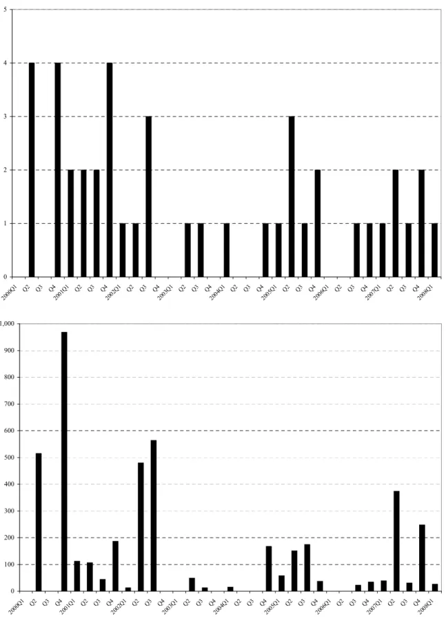
The average brokerage closure involves 103 stocks, with a maximum of 480 stocks. There are 2,181 unique stocks in the sample, so the average company is hit by two terminations over our sample period, with a maximum of 12. The 43 brokerage firms employed 557 analysts (not counting junior analysts without coverage responsibilities), so the average closure involved 13 analysts and the average analyst covered eight stocks. Sample terminations span all six-digit GICS industries (except REITs). The top graph in Figure 1 shows the quarterly number of brokerage closures. At least one brokerage firm exited research in 24 of the 33 quarters between Q1, 2000 and Q1, 2008, and there is no obvious evidence of the closures clustering in time.
The quarterly number of coverage terminations is shown in the bottom graph in Figure 1. Here, there is somewhat more evidence of clustering. Roughly half the terminations in the sample occurred in the first 2.5 years of the sample period, while there were virtually no terminations in the two years from Q4, 2002, a period during which many brokerage firms downsized their research operations with-out closing them completely (see Kelly and Ljungqvist (2008)). The largest number of terminations occurred in Q4, 2000, when four brokerage closures resulted in a total of 968 terminations.
Table I compares summary statistics for sample stocks, the CRSP universe of publicly traded U.S. stocks, and the universe of U.S. stocks covered by at least one analyst according to I/B/E/S. Sample stocks—like I/B/E/S stocks more generally—are on average larger than CRSP stocks. They are also somewhat more liquid and volatile than the average CRSP stock. On average, 10.6 analysts covered
a sample stock before a coverage termination, compared to 6.4 in the I/B/E/S database, suggesting that brokerage firms that exited research over our sample period disproportionately covered stocks with above-average analyst following. To the extent that less-covered stocks are proportionately more affected by a termination, this biases our tests against finding any effects.10
C. Announcement Dates
The relevant announcement date is the date investors learn that a brokerage has closed down its research department. We obtain these dates from Factiva. Both press releases and media reports are time-stamped, so we can pinpoint announcements with great precision.
It is important to note that information about a closure is freely available to all investors in a timely manner.11 Thus, both clients and other market participants can assess the implications, in terms of information asymmetry, for affected stocks and change their demands accordingly.
NYSE Rule 472(f)(5) and NASD Rule 2711(f)(5) require that clients are sent a termination notice every time a brokerage firm terminates coverage (including when it exits research completely). Termination notices must include the rationale for the termination, which removes any doubt, in our setting, that investors might misinterpret why coverage was terminated. The most common statement in our cases is simply that research has been closed down “based on our decision to exit the research business” (Wells Fargo termination notices, dated August 1, 2005).
D. Are Sample Terminations Exogenous?
Closure-related terminations constitute a suitably exogenous shock to the information environment
unless brokerage firms quit research because their analysts possessed negative private signals about the stocks they covered. Press reports around the time of the closure announcements make it clear 10Presumably, the increase in information asymmetry is greatest when a stock loses coverage entirely. Unfortunately, our sample contains only seven stocks that were ‘orphaned’ as a result of a closure-induced coverage termination.
11We find that the Dow Jones marketwatch.com service, which organizes its contents by ticker, typically reports news of a coverage termination the same day. Moreover, marketwatch.com provides a synopsis of the broker’s reason for the termination, allowing market participants to infer whether a stock was terminated for endogenous or exogenous reasons. In our case, the typical synopsis would relate a termination to the closure of the research operation.
that the closures are unlikely to have been motivated by negative information about individual stocks and so are plausibly exogenous. The following three examples illustrate.
Commenting on his decision to close down IRG Research, CEO Thomas Clarke blamed regulation: “With the brokerage industry facing some of the most far-reaching regulatory changes within the last 30 years, including S.E.C. rulings regarding the use of soft dollars and possibly the unbundling of research and trading costs, we could not see the economics working in our favor without substantial additional investment.” (Dow Jones, June 28, 2005)
Dutch bank ABN Amro closed its loss-making U.S. equities and corporate finance business, which included research, in March 2002. Among the 950 redundancies were 28 senior analysts who, along with junior team members, covered nearly 500 U.S. stocks. Board member Sergia Rial made it clear that the decision reflects competitive pressure and strategic considerations:
“We’re withdrawing from businesses in which we’re strategically ill-positioned and cannot create a sustainable profit stream, whether the market turns around or not.” (Chicago Tribune, March 26, 2002)
Regional broker George K. Baum closed its capital markets division, which included its research and investment banking operations, in October 2000, blaming a lack of profitability even during the booming late 1990s:
“Neither the retail brokerage nor equity capital markets divisions made money in the past two years.” (Knight Ridder Tribune Business News, Oct. 13, 2000)
These quotes suggest that brokerage firms quit research for strategic and financial reasons (often in the context of withdrawing from investment banking more generally) rather than to mask negative news about companies their analysts covered. Nonetheless, it is useful to test formally whether sample terminations are uninformative about the affected stocks’ future prospects.
D.1. Exogeneity Test
Suppose a broker terminates coverage at timet. If this signals private information about the stock, we should be able to predict its future performance from the fact that coverage was terminated. Testing
this requires an assumption about the nature of the signal. Assume that it is negative information aboutt+ 1 earnings that is not yet reflected in the consensus earnings forecast datedt−1 (i.e., before other analysts knew of the coverage termination). When earnings are eventually announced, they will fall short of thet−1 consensus, resulting in a negative earnings surprise. If, on the other hand, the termination is exogenous, earnings will not differ systematically from consensus.
This test is more powerful than simply checking whether terminations forecast changes in oper-ating performance (such as return on assets, ROA). By conditioning on consensus, the test exploits differences in the analyst’s and the market’s information sets under the null that the analyst has negative private information. Earnings surprises are ideal in this context because they are based on an observable forecast: surpriset+1 = EP St+1 −E[EP St+1|consensus infot−1]. For other measures
of operating performance, such as ROA, the market’s forecast is unobservable and must be estimated by the econometrician, which introduces noise and decreases the test’s power.
We implement the test in a large panel of CRSP companies over the period 2000 to 2008. Mirroring the construction of the terminations sample, we filter out companies with CRSP share codes greater than 12, leaving 5,823 CRSP firms and 96,455 firm-quarters. The dependent variable is the scaled earnings surprise, defined as (EP St+1−consensus f orecastt−1)/(book value of assets per sharet+1).
Earnings and forecast data come from I/B/E/S and book value data from Compustat.
The main variables of interest are two indicators. The first identifies the 4,429 terminations caused by the 43 brokerage closures. Its coefficient should be statistically zero if closure-induced terminations are uninformative about future earnings, and negative if our identifying assumption is invalid. The second identifies 10,349 firm-quarters in which the I/B/E/S stop file records that one or more brokers terminated coverage for reasons unrelated to a brokerage closure. We will refer to these as ‘endogenous’ terminations and expect a significantly negative coefficient. We control for lagged returns and return volatility measured over the prior 12 months, the log number of brokers covering the stock, and year and fiscal-quarter effects. We also add CRSP firm fixed effects to control for omitted firm characteristics and allow for auto-correlation in quarterly earnings surprises using
Baltagi and Wu’s (1999) AR(1)-estimator for unbalanced panels. This yields the following estimates:
earnings surprise = .607
.051return−0.053.276volatility −..120220log # brokers
−.267
.117endogenous termination +..172008sample termination+year effects
The firm fixed effects are jointly significant with an F-statistic of 4.2, and earnings surprises are significantly auto-correlated, withρ= 0.37.Standard errors are shown below the coefficients.
As expected, earnings surprises are significantly more negative following what we have labelled endogenous terminations (p = 0.022). The effect is large economically. On average, an endogenous termination is followed by a quarterly earnings surprise that is 16.5% more negative than the sample average over this period. Closure-induced terminations, by contrast, are neither economically nor statistically related to subsequent earnings surprises (p = 0.965). This is consistent with closure-induced terminations being uninformative about future performance and thus exogenous.
E. Do Coverage Terminations Increase Information Asymmetry?
Identification also requires that coverage terminations increase information asymmetry among in-vestors. To test whether they do, we examine changes around coverage terminations in three popular empirical proxies for information asymmetry: Bid-ask spreads, Amihud’s (2002) illiquidity measure, and Lesmond et al.’s (1999) illiquidity measure based on stale returns. We also examine changes in earnings surprises and return volatilities at future earnings releases, as these news events resolve a greater deal of uncertainty when information asymmetry is larger.
Throughout, we use difference-in-difference tests to help remove biases due to omitted variables or secular trends affecting similar companies at the same time (Ashenfelter and Card (1985)). To remove common influences, difference-in-difference tests compare the change in a variable of interest for treated firms to the contemporaneous change for a set of control firms matched to have similar characteristics but which are themselves unaffected by the treatment.
Given our focus on asset pricing, we follow Hong and Kacperczyk (2007) and match firms on the Fama-French (1993) pricing factors using the Daniel et al. (1997) algorithm. Specifically, we choose as controls for firm ifive unique firms in the same size and book-to-market quintile in the month of June prior to a coverage termination, subject to the condition that control firms did not themselves experience a termination in the quarter before and after the event. In view of the evidence from Table I that firms with coverage terminations are larger and more liquid than CRSP firms in general, we also require that controls be covered by one or more analysts in the three months before the event.
E.1. Results
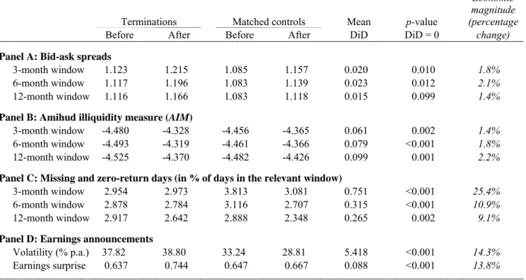
Table II, Panel A reports changes in bid-ask spreads around coverage terminations. If exogenous coverage terminations increase information asymmetry, we expect spreads to increase. For each stock, we compute the average bid-ask spread (normalized by the mid-quote) from daily data over three-, six-, or 12-month estimation windows ending 10 days before and starting 10 days after a termination announcement. Net of the change among control firms, spreads increase on average by 1.8%, 2.1%, and 1.4% over the three estimation windows, consistent with an increase in information asymmetry. For the first two windows, these changes are quite precisely estimated, with bootstrappedp-values of 0.010 and 0.012.12
Wang (1994) predicts that the correlation between absolute return and dollar volume increases in information asymmetry. This makes Amihud’s (2002) illiquidity measure (AIM) a natural proxy for information asymmetry, as it is defined as the log ratio of absolute return and dollar volume. Panel B reports changes inAIM. Relative to control stocks,AIM increases after a coverage termination for each estimation window, implying that the correlation between absolute return and volume increases as predicted. The increases are again economically meaningful. They average 1.4%, 1.8%, and 2.2% relative to the pre-termination means estimated for the three windows. They are also highly 12By construction, terminations cluster in time by broker. This poses a problem for standard cross-sectional tests, so we bootstrap the standard errors following Politis and Romano (1994). We reportp-values based on a block bootstrap with 10,000 replications and a block length of 100, the approximate average number of terminations per brokerage closure event.
statistically significant.
An alternative measure of illiquidity is due to Lesmond et al. (1999). A large number of zero-return or missing-zero-return days may indicate that a stock is illiquid. Panel C shows that net of the control-firm change, this number increases significantly following a coverage termination, by 25.4%, 10.9%, and 9.1% on average, measured over three-, six-, and 12-month windows, respectively.13
Panel D focuses on earnings announcements. Following coverage terminations, we expect returns to be more volatile around earnings announcements as more uncertainty is left unresolved (West (1988)). We also expect greater absolute earnings surprises, to the extent that post-termination consensus forecasts reflect coarser information sets. Consistent with these predictions, we find that log daily return volatility in the three days around earnings announcements increases by 14.3% net of the change among control firms (p < 0.001), while the average magnitude of absolute earnings surprises increases by 13.8% (p <0.001).
The evidence in Table II is consistent with the interpretation that information asymmetry increases following coverage terminations. In conclusion, sample terminations appear to be both uninformative about firms’ future prospects and correlated with changes in information asymmetry, as required for identification.
III.
The Effect of Information Asymmetry on Price and Demand
A. Change in Price
To test the first part of Proposition 1, we compute cumulative abnormal returns (CARs) from the close on the day before a termination announcement to the close on the announcement day [–1,0], one day later [–1,+1], or three days later [–1,+3]. Abnormal returns are computed using three benchmarks: The market model, the Fama-French three-factor model, and an industry benchmark. 13Note that the number of days with zero or missing returns actually declines for both treatment and control firms (presumably because markets are generally becoming more liquid in the wake of decimalization and competition from ECNs). However, the number declines relatively faster for control firms, so that the difference-in-difference statistics show a relative increase in illiquidity.
For the first two, factor loadings are estimated in a one-year pre-event window ending 10 days before the termination date. For the industry benchmark, abnormal returns are calculated as the simple difference between event-window cumulative returns for the sample stock and its corresponding Fama-French 30-industry portfolio.14
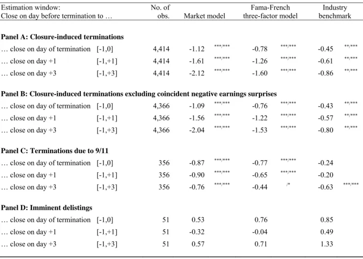
Table III, Panel A reports the results for the overall sample. Consistent with Proposition 1, price falls following the announcement of a coverage termination. On the day of announcement, CARs average−112,−78, and −45 basis points for the market model, the Fama-French model, and the industry benchmark, respectively (not annualized).15 If we measure announcement returns over
slightly longer windows through day +1 or day +3, CARs become more negative still, averaging up to −212 basis points. For the median sample firm, these price falls imply a fall in market value of between $4.6 and $21.6 million. In all cases, the point estimates are highly statistically significant using either a block bootstrap or a standard event-study test.
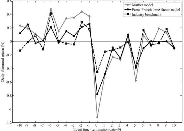
Figure 2 plots daily abnormal returns for trading days –10 through +10 relative to the day a brokerage firm closure was announced, for each of the three benchmarks. There is no evidence of abnormal returns before the announcements, consistent with the notion that the brokerage closures were unanticipated.16 On the announcement day, prices fall dramatically for each benchmark, and there is no evidence of a subsequent reversal over the next ten days. Though not shown in the figure, CARs continue to be negative even after one month, averaging −238, −220,and −129 basis points relative to the market model, the Fama-French model, and the industry benchmark, respectively. Each of these point estimates is significant at the 0.003 level or better. Thus, we find no evidence that the price falls are temporary.
Could confounding events be causing the price falls? If our terminations are truly exogenous, we 14Industry portfolio assignments are based on SIC codes; industry definitions, portfolio returns, and SIC mappings are taken from Ken French’s website.
15The fact that CARs are smaller when we use industry benchmarks suggests that there may be within-industry information spillover effects. Specifically, if stocks A and B suffer a coverage termination, the associated demand changes appear to affect stocks C and D in the same industry as well. This is a natural consequence of higher payoff correlations among stocks in the same industry (Veldkamp (2006b)).
16New reports confirm this. For example, when Wells Fargo closed its research department, one of the fired analysts was reported as saying, “We were told in a firm-wide announcement. I had no idea [it was coming].” (Wall Street Letter, August 5, 2005)
effectively have a randomized trial and so controls for confounding events are superfluous. Analysis of one particular confounding event, namely coincident negative earnings surprises, illustrates. First, we find that there are about as few coincident negative earnings surprises (1.09%) as chance alone would predict (1.26%).17 When these are excluded, average CARs are essentially unchanged: On the announcement day, for example, they are only two or three basis points higher (less negative) than in the full sample, ranging from −109 to−43 basis points for the three benchmarks.
As a reality check on our identification strategy, we turn to two alternative samples. The first comes from Keefe, Bruyette & Woods and Sandler O’Neill & Partners, two brokerage firms that suffered horrendous casualties in the September 11, 2001 terrorist attacks. Over the following three weeks, these two firms announced a total of 356 coverage terminations as the names of nearly 30 analysts killed in the World Trade Center were confirmed. Unlike the voluntary brokerage closures in our main sample, these terminations are clearly involuntary, and moreover, at the level of each analyst or affected stock, they are unquestionably random. Thus, if the 9/11 sample behaves similarly to the main sample, it is unlikely that brokerage firms timed their closure announcements in a way that would spuriously lead us to find a price fall.
Panel C reports the associated CARs. For the market model and the Fama-French model, CARs average −87 and −77 basis points on the announcement day (p <0.001), consistent with the results in our main model. Relative to the industry benchmark, CARs are also negative, but except for the [–1,+3] window, they are not statistically significant. We interpret these findings as support for Proposition 1. Overall, therefore, we find price falls following coverage terminations using two independent sources of identification, namely brokerage closures and 9/11.
Our second hold-out sample is designed to validate our identification strategy by contradiction. We return to brokerage closure-induced terminations but now focus on the 51 stocks—excluded from the main sample—that face imminent delisting within 60 days of a closure. For these stocks, a 17In the I/B/E/S universe, 39.72% of earnings surprises are negative over our sample period. With four earnings announcements, 252 trading days per year, and a two-day window, there is thus a 2·4/252·0.3972 = 1.26% chance that a coverage termination randomly coincides with a negative earnings announcement or the day before.
termination should be of little consequence because the asymmetric information increase over their remaining publicly traded lives is minimal in present value terms. Panel D reports the CARs. In contrast to the results shown in Panels A through C, CARs are generally small and positive rather than large and negative. The lack of statistical significance suggests that investors are unconcerned about a stock known to soon delist losing analyst coverage. This provides indirect support for our identification strategy.
B. Changes in Demand
According to Proposition 1, investors who choose to become privately informed following a coverage termination increase their holdings of the stock while those who become uninformed sell. Although we cannot identify directly who becomes privately informed, it seems plausible that retail investors are less likely to produce their own research than are institutional investors, which not only likely have a cost advantage in producing research themselves but often also maintain trading accounts with multiple brokerage firms and so face a relatively smaller loss of analyst information to begin with. We thus assume that a larger fraction of institutions than of retail investors becomes privately informed. Unfortunately, we have no high-frequency trading data to estimate changes in institutional and retail demand.18 Instead, we use the quarterly CDA/Spectrum data to compute the change in the fraction of a sample company’s outstanding stock held by institutions required to file 13f reports.19
Clearly, use of quarterly data will generate coarser and noisier results than the pricing results discussed in the previous section. As in Section II.E, we report difference-in-difference tests.
Panel A of Table IV shows that 13f filers as a group increase their holdings from 61.2% to 62.1% of shares outstanding following the average termination, with no contemporaneous change among control stocks. The average difference-in-differences is 0.9 percentage points, or 1.4% relative to the pre-termination average, with a bootstrapped p-value of 0.043. Thus, 13f institutions are unusually 18Trade size is sometimes used to infer retail trades, but decimalization in January 2001 and the growth in algorithmic trading mean that small trades are no longer viewed as a good proxy for retail trades.
19Investment companies and professional money managers with over $100 million under management are required to file quarterly 13f reports. Reports may omit holdings of fewer than 10,000 shares or $200,000 in market value.
large net buyers following terminations. If institutions are more likely to have low-cost substitute information sources than do retail investors, this result is consistent with Proposition 1.20
For robustness, Panel B provides similar evidence after excluding coincident negative earnings surprises. Panel C focuses on the 9/11 sample. Here, institutional holdings of affected stocks increase by 3.6% following a coverage terminations, though this point estimate is not statistically significant (possibly due to the small sample). Panel D shows that institutional holdings of stocks facing immi-nent delisting donot increase (in fact, they fall significantly) when coverage is terminated. As in the previous section, this provides indirect support for our identification strategy.
C. Testing the Comparative Statics
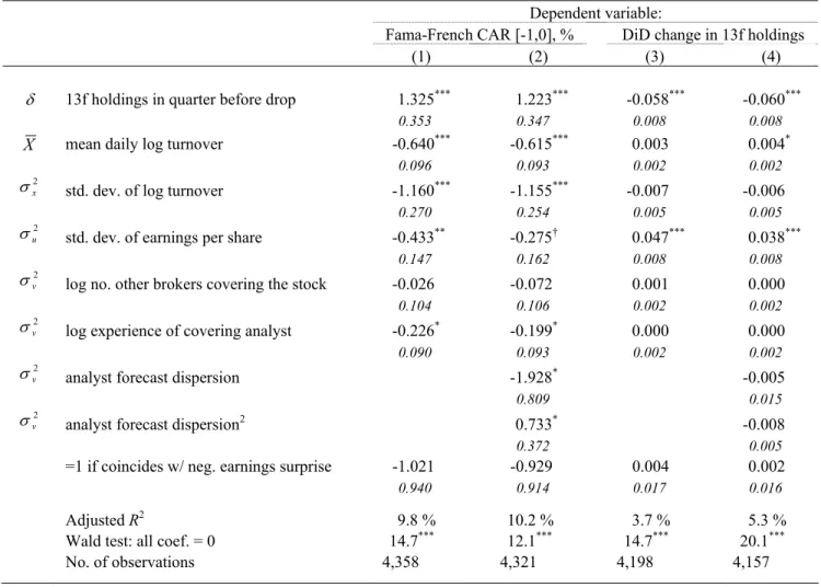
To test the comparative statics in Implications 1 through 4, we regress ∆EP and ∆EID on proxies for the five parameters of the model: δ (the fraction of informed investors), ¯X (mean aggregate supply), σ2
x (aggregate supply uncertainty), σ2u (payoff uncertainty), and σ2v (signal noise). We also
control for whether the termination coincides with a negative earnings surprise and for unobserved brokerage-firm specific effects using fixed effects. We use Fama-French announcement-day CARs to proxy for ∆EP21and the difference-in-difference change in institutional holdings to proxy for ∆EID. Our main proxy for δ is the fraction of the company’s stock held by institutional investors; call it ϕ. We do not claim that every institution will choose to become informed (i.e., that δ = ϕ). For the proxy to work, we only require that δ correlate positively with ϕ. This will be the case if institutions are more likely to become informed than retail investors, as argued earlier. We use the first two moments of the distribution of log daily share turnover to proxy for ¯Xandσ2
x, respectively.22
The proxy for payoff uncertainty σ2u is the standard deviation of quarterly earnings per share. We parameterize signal noiseσ2v as a function of the number of other analysts covering the stock and the quality of the analyst whose coverage is lost. Stocks covered by fewer analysts should have noisier 20By contrast, Xu (2006) finds that institutions reduce their ownership following endogenous terminations. Xu’s finding is consistent with the view that unlike our exogenous terminations, his endogenous ones are implicit sells.
21Results are robust to using market-model or industry-adjusted CARs and alternative estimation windows.
22An alternative proxy forX may be log free float. We prefer turnover because float captures the maximum possible supply while mean turnover better captures the typical supply actually observed.
signals, while high-quality analysts presumably produce more informative signals, so their coverage terminations should lead to larger price and demand changes.
Table V shows that the results generally support the comparative statics of the model. Columns 1 and 2 focus on changes in price. All coefficients have the predicted sign and all but one are statistically significant at the 5% level or better using bootstrapped standard errors to reduce the impact of clustering. We find that price falls are significantly larger in retail stocks (i.e., in stocks with smaller institutional holdings); the larger and more variable is turnover; the more volatile are earnings; and the more experienced is the analyst. The extent of coverage by other analysts and coincident negative earnings surprises are not significantly related to the magnitude of price falls. Economically, ∂∆EP/∂δ has the largest effect. A one standard deviation increase in our proxy for δ is associated with an additional price fall of 32.5 basis points, all else equal. The smallest effect comes from∂∆EP/∂σ2v (−5.6 basis points).
Recall that Implication 4 predicts a U-shaped relation between price changes and signal noise. When we include squares of the number of analysts covering the stock, or of the analyst’s experience, we find that neither is statistically significant. In column 2, we add an alternative proxy for signal noise, namely analyst forecast dispersion. We include both the level and square and find some support for a U-shaped relation: The coefficient for the level of forecast dispersion is negative (p= 0.017) while that for the squared term is positive (p = 0.049). However, the implied minimum is in the far right tail of the empirical distribution of forecast dispersion, so as a practical matter, in our data, ∆EP appears to decrease in all our proxies for signal noise.
Columns 3 and 4 repeat this analysis for changes in institutional holdings. The results are con-siderably noisier than those for changes in price—not surprisingly, given the quarterly nature of the 13f institutional ownership data we use to measure changes in informed demand. The signs for ∂∆EID/∂δ, ∂∆EID/∂X,¯ and ∂∆EID/∂σ2u are all as predicted and generally statistically signifi-cant. (Recall that the expected signs of the informed-demand effects are exactly opposite to those for the price effects.) None one of our proxies for signal noise is significant. We view these results as
encouraging, though given the obvious data limitations, they should be interpreted with caution.
D. Testing Corollary 2: Change in Expected Returns
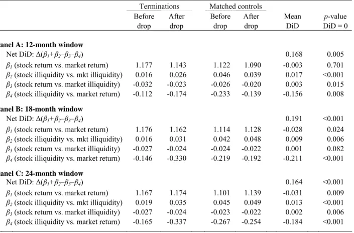
Falling prices following an increase in information asymmetry suggest that investors’ expected returns have increased. Corollary 2 states that expected returns increase because affected stocks become more sensitive to liquidity risk. To test this prediction, we estimate how a stock’s exposure to systematic liquidity risk changes following a coverage termination and relative to matched controls. Our empirical specification follows Acharya and Pedersen (2005) who propose an equilibrium model describing how exposure to aggregate liquidity risk affects a firm’s expected returns.23 Their pricing equation is
E(ri,t−rf,t) =E(ci,t) +λ(β1i+β2i−β3i−β4i) (7)
whereri,t is stock i’s month-treturn; rf,t is the riskfree rate; ci,t is a measure of stock i’s illiquidity;
λ is the price of risk; and the four betas measure exposure to aggregate risks, as embodied by the co-movement between: Stock returns and the market return (β1); stock illiquidity and aggregate illiquidity (β2); stock returns and aggregate illiquidity (β3); and stock illiquidity and the market return (β4).
The Acharya-Pedersen model captures the intuition that stocks should have lower prices (i.e., higher expected returns) when i) the stock return covaries more with the market return; ii) the stock’s illiquidity covaries more with aggregate illiquidity; iii) the stock return covaries less with aggregate illiquidity; and iv) the stock’s illiquidity covaries less with the market return. The first point is the CAPM rationale. The second assumes that an investor prefers stocks that are liquid when their portfolio is illiquid, all else equal. The third and forth points also capture this idea, noting that stocks with high returns in times of illiquidity, and stocks that are liquid when portfolio returns 23In a previous draft, we estimated factor models that included a liquidity factor and, like here, found that coverage terminations are followed by increased exposure to liquidity risk. We prefer the Acharya-Pedersen approach because it can be implemented over our entire sample period, 2000-2008. By contrast, data for the standard liquidity factors are available only through 2004 or 2005 (Pastor and Stambaugh (2003)) or 2006 (Sadka (2006)).
are low, should command high prices.
We estimate regression (7) separately for each stock i using weekly data over 12-month, 18-month, and 24-month windows ending two weeks prior to the termination announcement or starting two weeks after the announcement date. We focus on the weekly frequency to alleviate potential non-synchronicity concerns while providing enough data points in reasonably short windows to obtain reliable beta estimates.24 Aggregating over sample firms, we obtain mean betas before and after a
coverage termination. We repeat this procedure for control firms, selected as described previously, and compute difference-in-differences for each of the four betas. Equation 7 demonstrates that all betas are multiplied by the same price of risk. As a result, the effect of a termination on expected returns depends on the change in the total risk loading, (β1+β2−β3−β4). We provide a test of the mean total risk loading difference-in-difference, as well as for the individual beta changes.
The results, shown in Table VI, are consistent with Corollary 2. Regardless of estimation window, terminated stocks experience an increase in total risk loading of between 0.164 and 0.191, or 11.9% and 14.3% over their pre-termination means of 1.34 to 1.38. These point estimates are significantly different from zero using bootstrap tests to adjust for potential cross-sectional dependence due to time clustering of observations. The overall effect of these increased loadings is to increase the expected returns of stocks experiencing coverage terminations.
The increase in total risk loading is dominated by a significant drop in β4, representing an in-creased tendency for sample firms to experience poor returns in times of market illiquidity. Also, the comovement between market illiquidity and the illiquidity of sample stocks (β2) nearly doubles, with statistical significance. While unrelated to liquidity, we also find that post-termination returns load less strongly on the market factor (i.e., ∆β1 <0). Contrary to the model’s predictions, ∆β3 has a sign indicating decreased liquidity risk, in some cases significantly so. This effect, however, is economically 24A monthly frequency provides too few data points if we want to keep the estimation windows reasonably short to avoid confounding events. A daily frequency introduces a non-synchronicity problem. A common method to adjust for non-synchronous data is to include lags of independent variables and sum the loadings over all lags (see, for example, Scholes and Williams (1977)). However, construction of the Acharya-Pedersen illiquidity measure involves an adjustment for lagged aggregate market value. Including lagged independent variables therefore produces mechanical covariation between stock illiquidity and lagged market returns, used in calculatingβ4, so this non-synchronicity adjustment cannot be used. Using weekly data is therefore preferable.
small (averaging between 0.001 and 0.003) and is swamped by the liquidity risk increases captured by ∆β2 and ∆β4.
IV.
Conclusion
Asset pricing models routinely assume that investors have heterogeneous information, but it is an open empirical question how important information asymmetry really is for asset prices. This paper provides direct evidence of the effect of information asymmetry on asset prices and investor demands using plausibly exogenous variation in the supply of information.
The variation we exploit is caused by the closure of 43 brokerage firms’ research operations be-tween 2000 and the first quarter of 2008, which led to analyst coverage of thousands of stocks being terminated for reasons that we argue were unrelated to the stocks’ future prospects. Following such exogenous coverage terminations, information asymmetry increased (proxied by a range of standard measures such as bid-ask spreads), while share prices and uninformed (i.e., retail) investors’ demands fell. Consistent with the comparative statics of a Grossman and Stiglitz-type model, we find that the falls in price and uninformed demand are larger, the more investors are uninformed; the larger and more variable is turnover; the more uncertain is the asset’s payoff; and the noisier is the better-informed investors’ signal. We show theoretically that prices fall because expected returns become more sensitive to liquidity risk and provide empirical support for this prediction.
In sum, our results imply that information asymmetry has a substantial effect on asset prices and that a primary channel linking asymmetry to prices is liquidity. We believe that our quasi-experiment can serve as a useful source of exogenous variation for empirical work in other applications that examine the effects of information asymmetry in financial markets. In this spirit, we intend to make our set of exogenous coverage terminations available to fellow researchers.