HAL Id: hal-02167055
https://hal.archives-ouvertes.fr/hal-02167055
Preprint submitted on 27 Jun 2019
HAL
is a multi-disciplinary open access
archive for the deposit and dissemination of
sci-entific research documents, whether they are
pub-lished or not. The documents may come from
teaching and research institutions in France or
abroad, or from public or private research centers.
L’archive ouverte pluridisciplinaire
HAL, est
destinée au dépôt et à la diffusion de documents
scientifiques de niveau recherche, publiés ou non,
émanant des établissements d’enseignement et de
recherche français ou étrangers, des laboratoires
publics ou privés.
Online graph coloring with bichromatic exchanges
Sylvain Gravier, Marc Heinrich
To cite this version:
Sylvain Gravier, Marc Heinrich. Online graph coloring with bichromatic exchanges. 2019.
�hal-02167055�
Online graph coloring with bichromatic exchanges
Sylvain Gravier
1and Marc Heinrich
∗21
CNRS - Institut Fourier, Maths à Modeler, Grenoble, France.
2Université Lyon 1, LIRIS, France
June 27, 2019
Abstract
Greedy algorithms for the graph coloring problem require a large number of colors, even for very simple classes of graphs. For example, any greedy algorithm coloring trees requires Ω(logn) colors in the worst case. We consider a variation of greedy algorithms in which the algorithm is allowed to make modifications to previously colored vertices by performing local bichromatic exchanges. We show that such algorithms can be used to find an optimal coloring in the case of bipartite graphs, chordal graphs and outerplanar graphs. We also show that it can find colorings of general planar graphs withO(log ∆)colors, where∆is the maximum degree of the graph. The question of whether planar graphs can be colored by an online algorithm with bichromatic exchanges using only a constant number of colors is still open.
Keywords: online algorithms, graph coloring, bichromatic exchange, kempe chain.
1
Introduction
Online algorithms are a class of algorithms reading their input sequentially. In the case of graph problems, this usually means that the vertices of the graph arrive one by one. As the formal definition of greedy, online, and sequential algorithms is not completely fixed, we start by precising the convention we use here. In an online algorithm, for each new vertex, the algorithm must adapt a partial solution of the problem on the graph without the new vertex into a solution for the whole graph. For the graph coloring coloring problem, this means that, ifGis the graph andv the newly added vertex, the algorithm must
transform a coloring ofG−vinto a coloring of G.
A special class of online coloring algorithms which received a lot of attention is the class of greedy coloring algorithms, where the algorithm is not allowed to change his previous choices. The algorithm must assign a color to each new vertex that is different from the colors of its neighbors. Vertices colored at an earlier step cannot be recolored. The most common greedy algorithm for graph coloring isFirst-Fit,
where the color of the new vertex is taken to be the smallest color not already present in its neighborhood. These greedy algorithms are usually studied in a setting where the order on the vertices of the graph is arbitrary. The performance of these algorithms, is measured by the number of colors used for the worst case ordering.
A similar type of algorithms are sequential algorithms. These algorithms first decide on an ordering of the vertices, and then, apply an online algorithm to color the graph according to this ordering. In this case the ordering is chosen by the algorithm.
The greedy graph coloring problem is a widely studied subject. For general graphs, a randomized greedy algorithm finding anO( n
logn)approximation was devised in [Hal97] while there is a lower bound
ofΩ(logn2n)on the approximation ratio of any greedy algorithm. An important effort has been directed
at studying the performance on usual graph classes. A greedy algorithm with an approximation ratio of
O(logn) was shown for trees [GL88], bipartite graphs [LST89], planar and chordal graphs [Ira94]. On
the other hand, this approximation ratio was shown to be optimal for these graph classes [Bea76, AS17, LST89]. The lower bounds even holds for randomized algorithms, algorithms using a small reodering
buffer, or algorithm allowed to look at a few future inputs before making a choice [AS17]. Online algorithms with constant approximation ratio exists for other classes of graphs e.g. interval graphs [KT81, LV98, Smi10, NB08] and disk intersection graphs [CFKP07, EF02, AS17].
Since the approximation ratio of greedy algorithms is quite large even for some simple classes of graphs, it is natural to look at more general algorithms. In this article, we consider online algorithms which are allowed to change the color of previous vertices only by making local bichromatic exchanges. A bichromatic exchange (also called Kempe change in the litterature) consists in swapping the colors of the vertices of a maximal connected 2-colored subgraph of G. Applying this transformation creates a
new proper coloring of the graph. We call these algorithms online algorithm with bichromatic exchanges. For each new vertex v, the algorithm can perform bichomatic exchanges to remove one color from the
neighbors ofv, and use this color forv.
The choice of bichromatic exchanges as an operation to recolor the graph is quite natural. It was first considered in Kempe’s failed attempt at proving the four color theorem, and was used later to prove Vizing’s theorem [Viz64]. More recently, sequential algorithm using bichromatic exchange were considered in [MP99] to color a special subclass of perfect graphs, and in [HG96, HGM98, HM97, Tuc87] using more complex recolorings. In this context, bichromatic exchanges are used to locally modify an existing coloring in order to color a new vertex.
Finally, bichromatic exchanges were considered in the context of graph coloring reconfiguration. In this case the problem is, given two colorings of the same graph, to decide whether one can be transformed into the other by applying a sequence of basic operations. The case where the allowed transformation is to recolor a single vertex (a particular case of bichromatic exchange) has attracted a lot of attention. Some results were found for specific graph classes, for example chordal graphs [BJL+14] and graphs with
bounded treewidth [BB13, BB14]. Questions about the connexity of the reconfiguration graph [CVdHJ09, CVDHJ11] and some complexity aspects of the problem [BC09, CVDHJ11, JKK+14] have also been
considered. The case where the recoloring operations are bichromatic exchanges has been considered for planar graphs [Mey78, Moh06],K5-minor free graphs [LVM81] andd-regular graphs [FJP15, BBFJ15].
This last problem corresponds to a more global setting where the bichromatic exchanges can be applied anywhere in the graph. In our case, we are interested in local modifications of the coloring. This means that, as in sequential algorithms, the bichromatic exchanges are restricted to the neighborhood of the newly added vertex.
Overview. The paper is organized as follows. In the next section, we give standard notations, and a
formal definitions of online algorithm with bichromatic exchanges. Then, we describe such algorithms for several classes of graph: bipartite graphs in Section 2.1, chordal graphs in Section 3, outerplanar and planar graphs in Section 4. An extension of the algorithm on planar graphs to the case of graphs with bounded genus is presented in Section 5. Apart from the cases of planar graph and graphs with bounded genus, these algorithm are optimal and robust: they either find an optimal coloring or exhibit a forbidden substructure for this class of graphs. In the case of planar graph, the algorithm only provides a
log(∆)coloring, where∆is the maximum degree of the graph. The question of whether we can achieve a
constant number of colors is still open. Finally, in Section 6 we give an example of a family of3-colorable
graph for which any online algorithm using bichromatic exchanges (with some additional restrictions) performs badly.
2
Definitions and notations
We start with some standard definitions and notations of usual concepts from graph theory. A graph is a pair (V, E)where V is the set of vertices, and E, the set of edges, is a subset of unordered pairs of
distinct vertices. The graphs that we consider are simple, and undirected. Given a graph G= (V, E)
and a vertexv ofG, we denote byNG(v)the neighborhood ofv, i.e. NG(v) ={u∈V,{u, v} ∈E}, and
∆(G)the maximum degree of the graph G. When the graphGis clear from the context, we will omit
the subscript and just writeN(v)the neighborhood of v, and∆the maximum degree. If S is a subset
of vertices, we denote byG[S]the subgraph induced by all the vertices ofS.
A k-coloring of a graphG= (V, E)is a functionc:V 7→ {1, . . . , k} such that there is no
colori, we denote byci the set of vertices coloredi. In particular, for any two colors iandj, G[ci]is a
stable set, andG[ci∪cj] is the bipartite graph induced by vertices coloredior j.
Given a graphGand two verticesuandv, a path betweenuandv is a sequence of distinct vertices w0=u, w1, . . . , wk =v such that for all 0≤i < k, wi andwi+1 are adjacent in G. Given a coloringc
of G, and two colorsi and j, a path is a bichromatic (i, j)-path if every vertex of the path is colored
eitheri orj.
We look at a particular recoloring procedure called bichromatic exchange. A bichromatic exchange is a transformation that changes a coloring into a new one. Informally this recoloring is done by selecting a vertex, changing its color to a new color, and propagating the change to its neighbors to prevent the creation of monochromatic edges. We give a formal definition below:
Definition 1. Let Gbe a graph, v a vertex of G, and j a color. We denote byhv, ji the bichromatic
exchangethat transforms a coloringc of Ginto a coloringc0=hv, ji(c)defined by:
c0(x) = c(x) ifx6∈X c(v) ifx∈X andc(x) =j j ifx∈X andc(x) =c(v)
whereX is the connected component of G[cc(v)∪cj] containingv.
It is easy to check that this transformation does not create any monochromatic edges. From the definition, we can see that the color of a vertexuis changed by the bichromatic exchange hv, ii if and
only if there is a bichromatic(i, c(v))-path betweenuandv. LetS=hv1, i1i, . . . ,hvk, ikibe an ordered
sequence of bichromatic exchanges, andcbe a coloring. We denote byhSi(c) =hvk, iki◦. . .◦hv1, i1i(c)the
coloring obtained after applying successively the bichromatic exchanges ofS. In general, two bichromatic
exchanges do not commute, i.e. the order of application of several bichromatic exchanges is important. However, here are a few simple cases where they do commute:
Remark 1. Let Gbe a graph, cbe a coloring of G, andhx, ii,hy, jibe two bichromatic exchanges.
• If the colors i, j, c(x), c(y)are all different, thenhx, ii ◦ hy, ji(c) =hy, ji ◦ hx, ii(c).
• If i=j andc(x) =c(y), thenhx, ii ◦ hy, ji(c) =hy, ji ◦ hx, ii(c).
The algorithms that we consider are a special case of online algorithms where the algorithm is allowed to recolor previously colored vertices only by performing bichromatic exchanges. Allowing the algorithm to perform any bichromatic exchange would be too powerful as it would allow, in many cases, to recolor the whole graph. To prevent this, the algorithm is only allowed to perform bichromatic exchanges which are local to the newly added vertex in the following sense:
Definition 2. Let Gbe a graph,c a coloring ofG, andv, xtwo vertices ofG. The bichromatic exchange
hi, xiis local tov if x∈N(v).
We will always consider bichromatic exchanges which are local tov, the (not yet colored) vertex that
was just added to the graph. Consequently, we will omit to specifyv, and just write that the bichromatic
exchanges are local as a shorthand for local tov. Note that vertices outside the neighborhood ofvmight
be recolored by a local bichromatic exchange. Indeed, we only require that the starting point of a local bichromatic exchange is in the neighborhood ofv, but this transformation can still recolor a large part
of the graph. We can now give a formal definition of online algorithms with bichromatic exchanges.
Definition 3. An online coloring algorithm with bichromatic exchanges is an online algorithms such that, for each new vertexv:
• it applies a sequence of local bichromatic exchanges,
• and then selects a color forv not used by any vertex in its neighborhood.
This definition is quite general, however the algorithms that we will consider are more simple: they only perform bichromatic exchanges when necessary. If a color is already available to the new vertex without any recoloring, then the algorithm immediately selects that colors. Additionally, they always choose the smallest color available, and make no assumption on eventual properties of the existing
coloring. In other words, with these restrictions an algorithm with bichromatic exchanges is given by a procedure taking as input a graph G with a vertex v and any coloring c of G−v, and finding a
sequence of bichromatic exchanges such that applying these transformations removes one color from the neighborhood ofv.
In terms of graph coloring reconfiguration, the question this type of algorithms try to answer can be formulated in the following way. Given a graph G, a vertexv, and a k-coloring c of G−v, is there a
transformation ofcusing local bichromatic exchanges into a coloringc0for whichN(v)is(k−1)-colored.
Thus, the problem is similar to a coloring reconfiguration problem with two main variations: • the bichromatic exchanges must be local,
• the target coloring is not given, but can be any coloring with the desired properties.
An other important parameter for this kind of algorithm is the length of the reconfiguration path: the number of bichromatic exchanges that must be applied for each new vertex in the worst case. Since we are interested in only making local changes to the coloring, we want this number to be polynomial in∆.
The question we are interested in is to determine for which classes of graphs does such an algorithm exists and how many colors it requires. In the following, we will show several algorithms for different classes of graphs. Moreover, the algorithms that we will describe are robust in the following sense. For any graphG, if we run the algorithmA onG, then:
• either G∈ C, and Afinds a coloring ofG,
• or, Aexhibits a proof thatG6∈ C.
2.1
Bipartite graphs
The first simple class of graph that we might look at are bipartite graphs. We prove the following:
Theorem 2. There is an online coloring algorithm with bichromatic exchange finding a 2-coloring of
bipartite graphs using at most∆ operations at each step.
Proof. LetGbe the graph,va vertex ofG, andcthe coloring ofG−vobtained from the previous steps
of the algorithm. If one of the two colors is not present in the neighborhood ofv, then this color can be
used to colorv. Otherwise, the recoloring procedure is the following: while there is a vertexu∈N(v)
colored2, apply the bichromatic exchangehu,1i. None of the vertices inN(v)colored1can change color
back to2. Indeed, assume by contradiction that at some step a vertex w∈N(v)changes color from1
to2during the bichromatic exchange hu,1i. This implies that there is a pathpof odd length fromuto winG−v. Consequently,p∪ {v}is an odd cycle, a contradiction of the assumption thatGis bipartite.
When the procedure ends, after at most ∆ bichromatic exchanges, all the vertices in N(v) are
colored1, andv can be colored2.
In particular, this algorithm colors optimally any tree, while the best greedy online algorithm needs
Ω(logn)colors in the worst case.
3
Chordal graphs
In this section, we will exhibit an online algorithm with bichromatic exchanges that can color optimally any chordal graph. A chordal graph is a graph with no induced cycles of length larger than 3. They
have the following property:
Theorem 3 (Dirac, 1961). A graph G is chordal if and only if there is an ordering u1, . . . , un of its
vertices such that for alli≥1,N(ui)∩{u1, . . . , ui−1}is a clique. Such an ordering is called an elimination
ordering.
Such ordering can be computed in polynomial time. Chordal graphs are an important subclass of perfect graphs for which the chromatic number is equal to the largest clique in the graph. The idea of the algorithm is the following. Let v be the new vertex that was added to the graph. The algorithm
an elimination ordering of the vertices inN(v), and recolor these vertices one by one, according to this
ordering. The property that the whole graph is chordal will ensure that the colors of previously recolored vertices do not change during the successive operations. We first prove the following lemma:
Lemma 4. Let Gbe a graph, v a vertex of G, and c a coloring of G−v. Assume that there are two
vertices u1, u2 ∈N(v), such that there is a bichromatic (i, j)-path betweenu1 and u2 in G−v. If pis
the shortest such path, thenp⊆N(v).
Proof. Letu1 andu2 be two neighbors ofv such that there is a bichromatic(i, j)-path betweenu1 and
u2inG−v. Takepto be the shortest bichromatic(i, j)-path fromu1 tou2 for some colorsiandj. We
will show that p⊆N(v). Assume by contradiction that this is not the case, and there is at least one
vertex on the pathpwhich is not a neighbor ofv. We can find a subpathp0 ofpsuch thatp0 has length
at least2, and the only vertices ofp0 in N(v)are its two endpoints.
Since pis the shortest bichromatic(i, j)-path fromu1 tou2, the graph induced by p0 is a path, and
consequently, G[v∪p0] is a cycle of length at least4. This is a contradiction of the assumption thatG
is chordal.
Theorem 5. There is an online coloring algorithm with bichromatic exchange that colors optimally every chordal graph. The algorithm performs at most∆ bichromatic exchanges for each new vertex.
Proof. Given a graphH, we denote byω(H) the size of the largest clique in H. Let Gbe a graph, v
a vertex of G, andc a coloring of G−v using ω(G−v) colors. If ω(G) =ω(G−v) + 1, then we can
directly colorvusing the new additional color. Otherwise, let ω=ω(G). We will describe an algorithm
finding a sequence of bichromatic exchanges such that the resulting coloring uses at mostω−1 colors
onN(v). The transformation is made using at most∆bichromatic exchanges.
Since Gis chordal, the induced subgraphG[N(v)]is also chordal. Letk=|N(v)| be the number of
neighbors of v, and letv1, . . . , vk be an elimination ordering of the vertices ofN(v). We write Gi the
subgraph induced by the vertices v1, . . . , vi. The recoloring procedure is, for each i from 1 to k, if vi
is colored ω, we apply the bichromatic exchange hvi, xii where xi is the smallest color not present in
NGi(vi). There is always such a colorxi. Indeed, by definition of the order of the vertices, NGi(vi)is a
clique, andNGi(vi)∪ {vi, v} is also a clique ofG. Consequently,|NGi(vi)| ≤ω−2.
During step i, none of the verticesvj withj < iis recolored. Indeed, suppose by contradiction that
this is not the case, and let ibe the first step at which a vertexvj, withj < i is recolored. Before the
exchange, we havec(vj)6=ω. After the exchange, the color ofvj changes to ω. Consequently, there is
bichromatic(ω, xi)-path fromvi to vj inG−v. By Lemma 4, this implies that there is a bichromatic (ω, xi)-pathp⊆N(v)fromvi to vj.
Letvk be the vertex of the pathpwith the largest indexk. By choice of the color xi, we know that
vk 6=vi, since the (only) neighbor of vi in phas an index larger thani. Consequently, since j < i, the
vertex vk has two neighbors va and vb in p. Since p is2-colored, bothva andvb have the same color.
Additionally, by choice ofk, both a andb are smaller thank. Since the ordering of the vertices is an
elimination ordering, the neighbors ofvk inGk+1 form a clique. In particular, there is an edge between
va and vb, and this edge is monochromatic, a contradiction.
After the recoloring is done, none of the vertices ofN(v)is coloredω, and the colorωcan be assigned
tov.
4
Planar graphs
The goal of this section is to show two online algorithm with bichromatic exchanges. The first one allows to color outer-planar graphs using at most 3 colors. The second one can color any planar graph, but
only computes aO(log ∆)coloring. We start by the algorithm on outer-planar graphs.
4.1
Outer-planar graphs
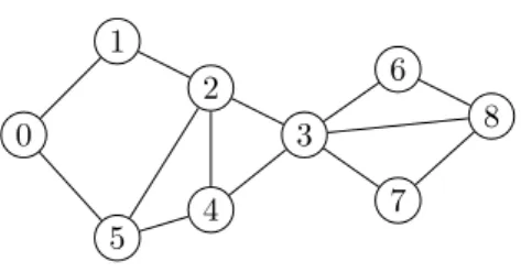
An outerplanar graph is a graph which admits a planar drawing such that there is a face adjacent to all the vertices of the graph. Such a drawing of an outerplanar graph can be computed in linear time [Bre77]. The face containing all the vertices of the graph is the outer-face. Given an outerplanar graphG, and
0 1 2 3 4 5 6 7 8
Figure 1: Example of outer-planar graph. The vertex3 appears twice on the outer face of the graph.
outer face. Note that the same vertex can appear several times in this sequence as in the example in Figure 1. We will prove the following Theorem:
Theorem 6. There is an online coloring algorithm with bichromatic exchange that colors optimally any outer-planar graph. The algorithm performs at most ∆bichromatic exchanges at each round.
Proof. Let Gbe an outer-planar graph, v a vertex of G, andc an optimal coloring of G−v. If G is
bipartite, then we can use the procedure from Theorem 2 to remove one color fromN(v), and obtain a 2-coloring of G. Otherwise, we can assume that the colors1,2and 3are present inN(v).
We will describe a procedure recoloringN(v)with only two colors using at most∆local bichromatic
exchanges.
Let k = |N(v)|, and let v0 =v, v1, . . . , vk be an ordering of the vertices ofN(v)∪v, in the order
they appear on the outer face in an outerplanar drawing of G. Note that there is no ambiguity in the
choice of this ordering. Indeed, suppose that there is a vertex, sayvi, that appears several times on the
outer-face. Then none of the vertices that appear between the first and last occurence ofvion the outer
face can be neighbors ofv, since it would contradict the fact thatGis outer-planar. We will recolor the
verticesv1, . . . , vk successively using the colors1 and2.
The algorithm recolors the vertices v1, . . . , vk in this order by doing the following. For i from 1 to
k, if c(vi) = 3, let x∈ {1,2} \ {c(vi−1)} (ifi = 1, x can be either1 or 2). We apply the bichromatic
exchangehvi, xi.
During step i, none of the vertices v1, . . . , vi−1 are recolored. Indeed, since G is outerplanar, any
path inG−vfromvito some vertexvjwithj < inecessarily goes throughvi−1. Additionnaly, the color
ofvi−1 is different fromxand3 by choice ofx. Consequently,vi−1 is not contained in any bichromatic
(x,3)-path, and there is no bichromatic (x,3)-path betweenvi and vj. At the end of this procedure,
N(v)is colored with colors1and 2, andv can be colored3.
4.2
General planar graphs
The case of general planar graph is more complicated, and we will only prove the following weaker theorem.
Theorem 7. There is an online algorithm with bichromatic exchanges coloring any planar graph with
O(log(∆))colors. The algorithm performs at most ∆22 bichromatic exchanges for each new vertex.
The question of whether there exists an algorithm using only a constant number of colors is still open. The algorithm is quite simple but the analysis is more complex than previous cases. The idea is to repeatedly apply a greedy procedure trying to remove one color from the the neighborhood of the new vertex v. We will show that when this greedy procedure cannot be applied any more, N(v) is colored
using at mostO(log ∆)colors.
We start by a few definitions. LetGbe a graph,v a vertex ofG, andca coloring ofG−v. Given a
colori, thesizeofiin the coloringcis the number of neighbors ofv coloredi: sizec(i) =|N(v)∩ci|. Let
hu, jibe a local bichromatic exchange, and letc0=hu, ji(c)andi=c(u). Suppose thatsizec(i)≤sizec(j).
The bichromatic exchange hu, ji is said to increase inequalities in c if we havesizec0(i)< sizec(i) and
sizec0(j) >size(j). Intuitively, a bichromatic exchange increases inequalities if it decreases the size of
colors with smaller sizes, and increases the size of color with larger sizes. The greedy recoloring procedure that we apply is the following.
Procedure(GreedyRecolor). While there is a local bichromatic exchangehu, iithat increases
To prove the theorem, we only need to prove two things: (i)the procedureGreedyRecolor ends in
a polynomial in ∆ number of rounds, and (ii)ifc is a coloring such that there is no local bichromatic
exchange increasing inequalities, thenN(v)is colored with at most O(log ∆)colors. The first point is
proved in the following Lemma 8. The second point will be proved in Lemma 10 in the next subsection.
Lemma 8. The procedureGreedyRecolorends after at most ∆22 rounds. Proof. To show this result, we will exhibit a potential functionΨsuch that:
• Ψincreases at every iteration of GreedyRecolor,
• Ψis upper bounded.
Letc be aK-coloring, we define the potentialΨ(c)by:
Ψ(c) = X
colori
(sizec(i))2.
We will show thatΨincreases by at least 2at each iteration of GreedyRecolor. Lethu, jibe a local
bichromatic exchange increasing inequalities inc, and leti=c(u)andc0 =hu, ji(c). By assumption on
hu, ji, we know thatsizec(i)≤sizec(j). Moreover, there is an integerxsuch that:
• sizec0(i) = sizec(i)−x
• sizec0(j) = sizec(j) +x
Sincehu, jiincreases inequalities, we havex≥1. Additionally, the following holds: Ψ(c0)−Ψ(c) = (sizec0(i))2+ (sizec0(j))2−(sizec(i))2−(sizec(j))2
= (sizec(i)−x)2+ (sizec(j) +x)2−(sizec(i))2−(sizec(j))2 = 2x2+ 2x(sizec(j)−sizec(i))≥2
Moreover Ψ(c) is upper bounded by ∆2 for any coloring c. Indeed, since we know that for any
coloringc,P
isizec(i) = ∆,Ψ(c)is maximum whensizec(i)is zero for all but one color. The potentialΨ
is positive, upper bounded by∆2, and increases by2at each iteration ofGreedyRecolor. Consequently,
the procedureGreedyRecolormust end after at most ∆22 rounds.
4.3
Grundy coloring of circular graphs
To prove the correctness of the algorithm described in previous subsection, we only need to show that if a coloring has no local bichromatic exchange that increases inequalities, then N(v) is colored using
at mostO(log ∆) colors. To prove this, we will use a result on a particular drawing of a graph which
could be of independent interest. We will first describe this construction, and prove that any coloring satisfying some properties related to this drawing uses a small number of colors. This will allow us to complete the proof of Theorem 7.
LetGbe a graph, with Gnot necessarily planar. A drawing ofGis a functionf that associates to
each vertex v of the graph a pointf(v)in the plane, and to each edge (u, v) of the graph a path from
f(u)to f(v). We call acircular drawing ofGa drawing of Gsuch that all the vertices are represented
by points on a circle, and the paths representing the edges are straight line segments.
Definition 4. LetG= (V, E)be a graph, with a drawing ofG. A proper coloringcof Gis intersection
compatibleif for any two crossing edges(u1, v1)and(u2, v2), the two sets{c(u1), c(v1)}and{c(u2), c(v2)}
intersect.
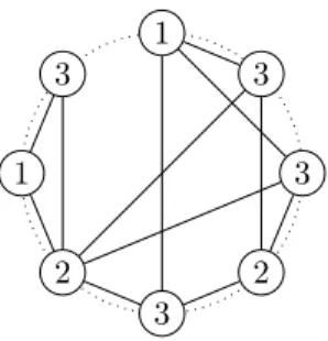
An example of a circular drawing of a graph with an intersection compatible coloring is given in Figure 2.
Not all graphsGhave a drawing with an intersection compatible coloring. Determining which graphs
have one could be an interesting question on its own. For example, there is no intersection compatible coloring ofK5, the clique on5vertices, for any of its drawing on a plane. On the contrary, any3-colorable
3 3 1 3 1 2 3 2
Figure 2: Example of circular drawing of a graph with an intersection compatible coloring. graph has one. In fact any 3-coloring of a3-colorable graph is intersection compatible for any drawing
of the graph, since in this case any two edges share at least one color.
Given a graphGwith a coloringc, the colored graph(G, c)will be called circular if there is a circular
drawing of Gthat makes the coloringcintersection compatible. A k-coloring c of a graph is aGrundy k-coloring if for every vertex u, and for every color j < c(u), there is a neighborw ∈N(u) such that
c(w) = j, and at least one vertex is colored k. In other words, every vertex is assigned the smallest
color that is not present in its neighborhood. The Grundy chromatic number of a graphGis the largest
number of colors ksuch that Ghas a Grundyk-coloring. To put it differently, a coloring is a Grundy
coloring if it can be obtained from the algorithmFirst-Fit, with a certain ordering of the vertices. The
Grundy chromatic number is the largest number of colors that the algorithmFirst-Fit might need for
the worst case ordering. We will prove the following result.
Lemma 9. There is a constantK0, such that for any circular colored graph (G, c) withn vertices, ifc
is a Grundy k-coloring ofG, thenk≤K0logn.
Note that the lemma does not prove that the Grundy chromatic number of a circular graph is at mostO(logn). Indeed, a circular graph could have a Grundy coloring using more colors. However, the
lemma states that in this case, this coloring is not intersection compatible.
Proof. We denote byT(k)the smallest number of vertices of a circular graphGhaving an intersection
compatible Grundyk-coloring c. To prove the lemma, it is enough to show that there are is a constant α >1such that T(k)≥αk−1 for anyk≥1. We takeα= 214, and show this inequality by induction on k. Ifk≤4, we know thatT(k)≥k≥αk−1.
Let us assume thatk >4, and let(G, c)be a colored circular graph withT(k)vertices such thatcis
a Grundyk-coloring. Letu0 be a vertex coloredk. Sincecis a Grundy coloring, there are three vertices
u1, u2, andu3adjacent tou0such that for eachi∈ {1,2,3},uiis coloredk−i. Letv0=u0, v1, v2, v3 be
the vertices{u0, u1, u2, u3} in the order they appear on the circle in the corresponding circular drawing
ofG. We denote byG0 the subgraph induced by the vertices with a color at most k−4. We will show
thatG0 is composed of at least2connected components, each of which contains all the colors from1 to
k−4. By applying the induction hypothesis on each of these components, this gives as needed:
T(k) =|G| ≥ |G0| ≥2·T(k−4)≥2·αk−5=αk−1.
Thus, we only need to show that G0 contains at least two connected components, each of which
contains all the colors from 1 to k−4. Since c is a Grundy coloring and c(v1) > k−4, there is a
vertex w1 adjacent tov1 with c(w1) =k−4. Similarly, there is a vertex w2 adjacent tov3 with color
c(w2) = k−4. See Figure 3 for an illustration. Let G1 and G2 be the connected components of G0
containingw1 andw2 respectively. Then G1 =6 G2. Indeed, if w1 and w2 were in the same connected
component of G0, then there would be a path from w
1 to w2 using only colors less than or equal to
k−4. By adding the two edges(v1, w1)and(v3, w2), we would obtain a path fromu1tou3 which does
not use the colors k = c(v0)and c(v2). However, this path must necessarily cross the edge (v0, v2), a
contradiction of the assumption that the coloringc is intersection compatible.
Consequently we have T(k) ≥αk−1 which can be rewritten ask ≤ 1 + log(log(T(αk))) ≤K0log(n) with
v0 v1
v2
v3
G1
G2
Figure 3: Any edge crossing the edge (v0, v2) must have either c(v0) or c(v2) as the color of one of
its endpoints. Since G0 contains no vertex with color c(v0) or c(v2), G0 is split into two connected
components, one on each side of the edge(v0, v2).
We can now see how to use the previous result to complete the proof of the algorithm on planar graphs. The following lemma is the only remaining missing part to prove Theorem 7.
Lemma 10. Let Gbe a planar graph, v a vertex of G, and c a coloring of G−v. If there is no local
bichromatic exchange that increases inequalities,N(v)is colored using at mostK0log ∆ colors for some
constant K0.
Proof. We build the graph G0 as follows. The set of vertices of G0 is N(v), the neighbors of v. For
every pair of verticesu1, u2∈N(v)such thatc(u1)=6 c(u2), we add the edge (u1, u2)inG0 if there is a
bichromatic path fromu1 tou2inG. We consider a circular drawing ofG0where the vertices appear on
the circle in the order they appear around the vertexv in a planar drawing ofG.
The coloring cofGinduces a coloringc0 ofG0 such that:
• The coloringc0 is proper. Indeed, we only added edges inG0 between vertices with different colors.
• The coloring c0 is intersection compatible. Let (u
1, u3) and (u2, u4) be two crossing edges in
G0. Then, the vertices ui appear with the order u1, u2, u3, u4 around the vertexv in the planar
drawing of G. Additionally, there is a bichromatic(c(u1), c(u3))-pathp1 in Gfrom u1 to u3, and
a bichromatic (c(u2), c(u4))-path p2 from u2 to u4. Since G is planar, p1 and p2 must cross at
some vertex w. This implies that c(w) ∈ {c(u1), c(u3)} ∩ {c(u2), c(u4)}, and consequently, this
intersection is not empty.
• Finally, assume that the colors are ordered 1, . . . , k such that sizec(1)≥sizec(2)≥. . .≥sizec(k).
Then c is a Grundy coloring of G0 for this ordering of the colors. Indeed let u be a vertex of G0, and assume by contradiction that there is a vertexuand a colori < c0(u)such that uhas no
neighbor coloredi. Then consider the bichromatic exchangehu, iiin the graphG. This bichromatic
exchange does not change the color of any neighbor ofv coloredi. And since we havei < c(u), this
implies size(i)≥size(u). Performing the bichromatic exchangehu, iiwould increase the size of i,
and decrease the size ofc(u). Thushu, iiincreases inequalities, a contradiction of the assumption
that cdid not contain any bichromatic exchange increasing inequalities.
By applying Lemma 9 on the graph G0 with the coloringc0, we obtain that there is a constant K 0
such thatc0 uses at mostK0log ∆ different colors. Consequently, the coloringc uses at mostK0log ∆
colors onN(v).
We now have all the ingredients to prove the theorem.
Proof of Theorem 7. LetK0be the constant in Lemma 10. The algorithm usesK0log ∆ + 1colors. For
each new vertex v, the procedure GreedyRecolor is applied on N(v). By Lemma 8, the procedure
performs at most ∆2
2 of bichromatic exchanges. After the procedure has ended, we obtain a coloringc 0
such that there is no local bichromatic exchange that increases inequalities. By Lemma 10, this implies thatc0 colors N(v)using at mostK0log ∆colors. Consequently, the algorithm colors any planar graph
5
Graphs of bounded genus
In this section, we show that the algorithm we described above can be adapted to the case of graphs with bounded genus, by only paying a small additional number of colors. We start by some very quick notations. We will assume that the reader is familiar with basic notions of topology and surfaces with boundaries. An introduction to these notions can be found for example in chapter4from [Ada04].
Given a triangulation T of a surface S, we denote by V(T), E(T) and F(T) the set of vertices,
edges and faces respectively of the triangulation T. Let S be a surface with a triangulation T. The
Euler characteristic of S is the quantity|V(T)| − |E(T)|+|F(T)|. This quantity is an invariant of the
surface S that is preserved by homeomorphism, and is independent of the chosen triangulation. The
Euler characteristic can be negative, and is at most2 for a connected closed surface, and at most1 for
a connected surface with boundary. For an orientable surfaceS, the genus gofS is related to its Euler
characteristichby the formula h= 2−2g.
A drawing of a graphGon a surfaceSis a mappingf that associates to every vertexv ofG, a point f(v)onS, and to every edge(u, v)ofG, a path onSfromf(u)tof(v). An embedding of a graphGon S is a drawingf ofGon the surfaceS such that for any two edgese1 ande2, the pathsf(e1)andf(e2)
do not intersect. In the following, the Euler characteristic (resp. genus) of a graph Gwill denote the
largest number h(resp. smallest number g) such that there exists an embedding ofG on a connected
surface S with Euler characteristic h(resp. genus g). Planar graphs have Euler characteristic 2 and
genus0. The goal of this section is to show the following theorem:
Theorem 11. There is an online algorithm with bichromatic exchanges that can color any graph with Euler characteristichusing 5−2h+O(log ∆) colors.
The algorithm is exactly the same as for the planar case. To remove one color from the neighborhood of a vertexv, we just apply the procedureGreedyRecolor. Thus, to prove the correctness of the
algo-rithm, we only need to show that, when there is no more bichromatic exchanges increasing inequalities, the neighborhood of thev is colored using at most4−2h+O(log ∆)colors.
To prove this result, we generalize the definition of circular graph from previous section to handle graphs drawn on surfaces with higher genus. LetS be a surface with boundary, and Gbe a graph. A
boundary drawing of G onS is a drawing f of G on the surfaceS such that for every vertex v, f(v)
is on the boundary ofS. In a boundary drawing, paths corresponding to different edges are allowed to
intersect. In particular, ifS is a disk, a boundary drawing of a graphGonS is a circular drawing ofG.
The definition of intersection compatible coloring extends to boundary drawings in a natural way. If
Gis a graph with a boundary drawingf on a surface S, a coloringc ofGis intersection compatible if
for every pair of edges e= (u, v) and e0 = (u0, v0), if the paths f(e) and f(e0)intersect, then the two
edges have at least one color in common, i.e.,{c(u), c(v)} ∩ {c(u0), c(v0)} 6=∅. We will need the following
simple result describing how the Euler characteristic of a surface changes when we cut this surface along a path.
Lemma 12. Let S be a surface with a boundary, and p be a simple path on S between two boundary
points. Cutting the surface S along the pathpyields a surface with Euler characteristic increased by1.
Proof. LetS be a surface with boundary, andhthe Euler characteristic ofS. Letpbe a path between
two boundary points of S, and S0 be the surface obtained by cutting S along the path p. Let T be
a triangulation of S. Without loss of generality, we can assume that the path pis along the edges of
the triangulationT. Consider the triangulationT0 where each edge and each vertex of the pathpwere
duplicated as in Figure 4. Letnbe the number of vertices in the pathp. Then,T0 is a triangulation for S0, and the Euler characteristic ofS0 is:
|V(T0)| − |E(T0)|+|F(T0)|= (|V(T)|+n)−(|E(T)|+n−1) +|F(T)|=h+ 1
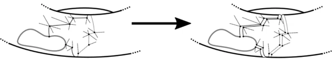
Note that in some cases, cutting a surface along a path can disconnect the surface, or increase the number of boundary components as in Figure 4. To prove the theorem, the key ingredient is to prove an extension of Lemma 9 for graphs with a boundary drawing on an arbitrary surface. This is done in the following lemma.
Figure 4: Cutting a surface (here a torus with a boundary) along a path. The bold grey line is the boundary of the surface.
Lemma 13. There exists a constant K0 such that, if G is a graph with n vertices with a boundary
drawing on a surface S with Euler characteristic h, and c is a Grundy k-coloring of G which is also
intersection compatible, thenk≤K0logn+ 2(1−h).
Proof. We show the result by induction onh, the Euler characteristic of the surfaceS. Ifh= 1, then
the surfaceS is a disk, and the result follows from Lemma 9. Suppose thath <1, and letGbe a graph
with a boundary drawingf on a surfaceS with Euler characteristich. Letcbe a Grundy coloring ofG
that is intersection compatible for this drawing. We distinguish two cases:
Case 1. There is an edgeeofGsuch that cutting the surfaceSalong the pathf(e)leaves the surface
connected. Let a and b be the two colors of the endpoints of this edge. We consider S0, the surface
obtained by cuttingS alongf(e), andG0 the graph induced by the vertices with a color different from
a or b. Then, the boundary drawing of G on S induces a boundary drawing of G0 on S0. Indeed, if
(u, v)is an edge ofG0, then the path corresponding to(u, v)cannot crossf(e)since otherwise one of the
endpointsuorv would be colored eitheraor bsince the coloring is intersection compatible.
Moreover, by Lemma 12, the surfaceS0 has Euler characteristich+ 1. Using the induction hypothesis
onG0, with the coloring induced byconG0, we know thatccolorsG0with at mostK0logn+2(1−(h+1))
colors. Since the vertices we removed were the ones coloredaorb, this implies that the coloring cofG
uses at mostK0logn+ 2(1−h)colors, which proves the induction step.
Case 2. For any edge e, cuttingS along the pathf(e)disconnects the surface. In this case, we claim
that the graphGhas a boundary drawing on a disk such thatcis intersection compatible for this drawing.
To prove this, we first remark that we can assume that there is only one boundary component on the surfaceS. Indeed, suppose that this is not the case. Consider the boundary that contains a vertexvwith
colork, the largest color used by c. Let G0 be the graph induced by all the vertices on this boundary.
Then all the colors are present inG0. Indeed,G0 contains the vertexvwith colork. Sincecis a Grundy
coloring, there are verticesv1, . . . , vk−1adjacent tov, with colors1, . . . , k−1 respectively. For alli, the
vertexvi is on the same boundary asvsince otherwise cutting along the path corresponding to the edge (v, vi)would leave the surface connected. Let c0 be the coloring induced byc onG0. If the result holds
forG0 with coloringc0, it also holds for Gwith coloringcsincecand c0 use the same number of colors.
So we now assume thatS has one unique boundary.
Letu1, . . . , un be the vertices of Gin the order they appear on the boundary of S, and consider the
circular drawing ofGusing the same orderingu1, . . . , un around the circle. To prove the result, we only
need to show thatc is also intersection compatible for this new drawing. Indeed, if this is the case, then
the result immediately follows from Lemma 9. Let e1 and e2 be two edges of G that intersect in the
circular drawing of G. Without loss of generality, we can assume that e1 = (u1, ui), ande2 = (uj, ul),
with 1 < j < i, and i < l ≤n. Let p1 and p2 be the paths on S corresponding to these two edges.
Assume by contradiction that in the drawing of GonS, the two paths p1 andp2 do not intersect, we
will show that cutting alongp1 does not disconnect the surface S. For this, it is enough to show that
there is a path not intersectingp1 going from one side ofp1 to the other side. We will construct a path
from ui−1 to ui+1 that does not intersect p1. The path is as follows. Go from ui−1 to uj by following
the border ofS, then follow the pathp2fromuj toul, and finally go fromultoui+1 by following again
the border ofS. This path does not intersectp1. Hence cutting alongp1 leaves the surfaceS connected,
a contradiction.
Thus, we know that for every pair of edges e1 ande2, if the segments corresponding toe1 ande2in
GonS also intersect. Consequently,cis intersection compatible for this circular drawing ofG, and the
result follows from Lemma 9.
We now have everything we need to prove the theorem.
(proof of Theorem 11). The proof follows the same argument as the proof of Theorem 7. Let G be a
graph with Euler characteristich,va vertex ofG, andca coloring ofG−v. We want to show that after
applying procedureGreedyRecolor, the neighborhood ofvis colored using at mostK0log ∆ + 2(2−h)
colors. Let S be a closed surface with Euler characteristic hsuch that there is an embedding of Gon S. Let G0 be the graph whose vertices are the neighbors ofv, and such that there is an edge between u1 andu2 if and only if c(u1)=6 c(u2)and there is a bichromatic path from u1 tou2. Without loss of
generality, we can assume that the colors are ordered by decreasing size: sizec(1)≥sizec(2)≥. . .. Then,
as before, c is a Grundy coloring ofG0. Indeed, if there is a vertex v and a color i < c(v) such thatv
has no neighbor coloredi, then the bichromatic exchangehv, iiincreases inequality.
Moreover, if S0 is the surface S where a small disk around vertex v was removed, then from the
embedding of G on S, we can construct a boundary drawing of G0 on S0. The coloring c induces an
intersection compatible drawing ofG0 for this drawing. Since the Euler charactersitic of S0 ish−1, by
Lemma 13, at most K0log ∆ + 2(2−h) are used by c on G0. Consequently, at least one color is not
present in the neighborhood ofv.
6
Counter example
The goal of this section is to exhibit concrete example of graphs with small chromatic number that need a large number of colors to be colored by an online algorithm using bichromatic exchanges. Unfortunately, this example does not work for general algorithms with bichromatic exchanges, but only to more special cases with the following restrictions on the algorithm:
• The algorithm is specified as input the number kof colors it is allowed to use to color the graph.
• If one of thekcolors is available, the algorithm must select it, without performing any bichromatic
exchange.
• The algorithm always chooses the smallest color available.
These assumptions might seem a bit restrictive, but all the algorithms we described above satisfy these constraints. Getting a counter example that would work in the general case is more complicated as it is difficult to quantify how much the graph can be recolored by bichromatic exchanges performed by the algorithm. We show the following theorem:
Theorem 14. There is a sequence of graph(Gk)k≥0 such that for all k≥4,Gk is3 colorable, and no
online algorithm with bichromatic exchanges with the restrictions above can color Gk with k colors or
less.
Proof. Let A be an online algorithm with bichromatic exchanges with the restrictions above. First
observe that as long as one color is available, the algorithmA behaves exactly asFirst-Fit: it assigns
the smallest color available without changing the color of previously colored vertices. We denote byTk
the fibonacci tree with the following definition. The tree T1 is a single vertex, and for k > 0, Tk is
composed of a root vertexu, to which we attach the treesT1, . . . , Tk−1.
It was proved in [Bea76], that if the vertices of Tk are presented starting from the leaves, and going
up to the root, then First-Fit needsk colors to color Tk, and the root of Tk is colored with color k.
We build the graphHk in the following way:
• for each 1≤i≤k, we add a copy ofTi, with vertexui as the root,
• for eachi < j, and each i06=iand j06=j withi0 6=j0, we add one copy ofTi0 and one copy ofTj0
with rootsw1
i,j,i0,j0 andwi,j,i2 0,j0 respectively,
• finally, a vertexuis added, withuadjacent to all theui.
The graphHk is presented starting from the leaves of all the copies ofTi, and going up to the roots.
The vertexuis presented last. SinceHk is2-degenerate, it is3 colorable. We prove that the algorithm
A can’t colorHk if it is given exactly kcolors. Indeed, since the algorithm always color immediately a
vertex if one color is available, it will be able to color all the vertices except foru, by applying the rules
ofFirst-Fit. When it tries to coloru, all the colors are already present in the neighborhood ofu, so the
algorithm might try to remove one color using local bichromatic exchanges. However, we will show that at this point, no local bichromatic exchange can remove one color from the neighborhood of u. More
precisely, we will show that any local bichromatic exchange will preserve the following invariants: 1. The verticesui all have different colors.
2. For every indices iandj, withi6=j, and every pair of colorsa6=b witha6=c(ui), andb6=c(uj),
there is a path on four vertices(ui, w1, w2, uj)such thatc(w1) =aandc(w2) =b.
By construction, these invariants are satisfied before any bichromatic exchange is made. Suppose now that there is a coloringc that satisfies these invariants. Consider the bichromatic exchangehui, xi,
and let j 6= i such that x=c(uj). We will show that the coloring c0 =hui, xi(c)still satisfy the two
invariants above.
Using the fact that c satisfies the second invariant, we know that there is a bichromatic path from ui to uj. Consequently, applying the bichromatic exchange hui, xi, swaps the colors of the verticesui
and uj. Consequently,c0 still satisfies the invariant 1. We only need to show that c0 also satisfies the
second invariant. Consider two indicesi0 and j0, and two colorsa6=c0(i0) andb 6=c0(j0). We consider
the following three cases:
• Ifi0 6=iandj0 =6 j, thenc0(ui0) =c(ui0)andc0(uj0) =c(uj0). Sincecsatisfies the second property,
there are two vertices w1and w2 such thatc(w1) =a andc(w2) =b such that(ui0, w1, w2, uj0)is
a path on four vertices. Since the colors ofw1and w2 also do not change during the bichromatic
exchange, we also have c0(w1) =aandc0(w2) =b.
• If i0 =i and j0 6= j, thenc0(ui) = c(uj), and c0(uj0) =c(uj0). If a 6=c(uj), then in the coloring
c there was a path on four vertices with successive colors (c(ui), a, b, c(uj0)). This path now has
colors(c(uj), a, b, c(uj0)). Ifa=c(ui)andb6=c(uj), then with the coloringcthere was a path from
ui to uj0 with colors (c(ui), c(uj), b, c(uj0)). This path is now colored (c(uj), a= c(ui), b, c(uj0)).
Finally, if a = c(ui) and b = c(uj), the path with colors (c(ui), c(uj), c(ui), c(uj0)) now has the
necessary colors.
The argument is symmetrical ifi0 6=iandj =j0.
• If i0 =i and j0 = j, the same argument as above can be used to prove that there is still a path
betweenui anduj with colors(c0(ui), a, b, c0(uj)). The idea is that colors different thanc(ui)and
c(uj)are unchanged, and vertices coloredc(ui)orc(uj)gets their color swapped.
Consequently, the invariant is preserved when we perform any local bichromatic exchange. Conse-quently, the algorithmAwon’t be able to colorHk if it is given exactlykcolors. However, the argument
relies on the fact that the algorithm does not perform bichromatic exchanges before considering the vertex u. Consequently, the algorithm might still manage to color Hk if it is given less than k colors.
This issue can be solved by consideringGk=Si≤kHi. For anyk0 ≤k, the algorithmAwill fail to color
Hk0, and consequentlyGk, and the theorem holds.
7
Conclusion
We studied a variation of online algorithms where the algorithm is allowed to recolor some of the pre-viously colored vertices. We have shown algorithms for several classes of graphs. In the case of planar graphs, it remains open whether theO(log ∆)bound can be improved or not.
We introduced the notion of intersection compatible coloring which could be interesting to look at on its own. In particular, a relevant question could be to try to characterize the graphs which have a drawing on a given surfaceS such that any two intersecting edges share a common color.
Finally, from an reconfiguration point of view, we studied a recoloring problem with some locality constraints on the transformations that we are allowed to make. It could be interesting to look at standard reconfiguration problems when we add these constraints. An example of problems to look at could be, deciding if a given coloring can be transformed into an other using local bichromatic exchanges, or given two vertices uand v, deciding if there is a sequence of bichromatic exchanges local to u that
change the color ofv.
References
[Ada04] Colin Conrad Adams.The knot book: an elementary introduction to the mathematical theory of knots. American Mathematical Soc., 2004.
[AS17] Susanne Albers and Sebastian Schraink. Tight Bounds for Online Coloring of Basic Graph Classes. In Kirk Pruhs and Christian Sohler, editors, 25th Annual European Symposium on Algorithms (ESA 2017), volume 87 of Leibniz International Proceedings in Informatics (LIPIcs), pages 7:1–7:14, Dagstuhl, Germany, 2017. Schloss Dagstuhl–Leibniz-Zentrum fuer Informatik.
[BB13] Marthe Bonamy and Nicolas Bousquet. Recoloring bounded treewidth graphs. Electronic Notes in Discrete Mathematics, 44:257–262, 2013.
[BB14] Marthe Bonamy and Nicolas Bousquet. Recoloring graphs via tree decompositions. ArXiv preprint arXiv:1403.6386, 2014.
[BBFJ15] Marthe Bonamy, Nicolas Bousquet, Carl Feghali, and Matthew Johnson. On a conjecture of mohar concerning kempe equivalence of regular graphs. ArXiv preprint arXiv:1510.06964, 2015.
[BC09] Paul Bonsma and Luis Cereceda. Finding paths between graph colourings: Pspace-completeness and superpolynomial distances. Theoretical Computer Science, 410(50):5215– 5226, 2009.
[Bea76] Dwight R Bean. Effective coloration. The Journal of Symbolic Logic, 41(2):469–480, 1976. [BJL+14] Marthe Bonamy, Matthew Johnson, Ioannis Lignos, Viresh Patel, and Daniël Paulusma.
Reconfiguration graphs for vertex colourings of chordal and chordal bipartite graphs.Journal of Combinatorial Optimization, 27(1):132–143, 2014.
[Bre77] Wayne M Brehaut. An efficient outerplanarity algorithm. In Proceedings of the 8th South-Eastern Conference on Combinatorics, Graph Theory, and Computing, pages 99–113, 1977. [CFKP07] Ioannis Caragiannis, Aleksei V Fishkin, Christos Kaklamanis, and Evi Papaioannou. A tight bound for online colouring of disk graphs. Theoretical Computer Science, 384(2-3):152–160, 2007.
[CVdHJ09] Luis Cereceda, Jan Van den Heuvel, and Matthew Johnson. Mixing 3-colourings in bipartite graphs. European Journal of Combinatorics, 30(7):1593–1606, 2009.
[CVDHJ11] Luis Cereceda, Jan Van Den Heuvel, and Matthew Johnson. Finding paths between 3-colorings. Journal of graph theory, 67(1):69–82, 2011.
[EF02] Thomas Erlebach and Jiri Fiala. On-line coloring of geometric intersection graphs. Compu-tational Geometry, 23(2):243–255, 2002.
[FJP15] Carl Feghali, Matthew Johnson, and Daniël Paulusma. Kempe equivalence of colourings of cubic graphs. Electronic Notes in Discrete Mathematics, 49:243–249, 2015.
[GL88] András Gyárfás and Jenö Lehel. On-line and first fit colorings of graphs. Journal of Graph theory, 12(2):217–227, 1988.
[Hal97] Magnús M Halldórsson. Parallel and on-line graph coloring. Journal of Algorithms, 23(2):265–280, 1997.
[HG96] Hacène Ait Haddadene and Sylvain Gravier. On weakly diamond-free berge graphs.Discrete Mathematics, 159(1-3):237–240, 1996.
[HGM98] Hacène Aït Haddadène, Sylvain Gravier, and Frédéric Maffray. An algorithm for coloring some perfect graphs. Discrete mathematics, 183(1-3):1–16, 1998.
[HM97] Hacène Aït Haddadène and Frédéric Maffray. Coloring perfect degenerate graphs. Discrete Mathematics, 163(1-3):211–215, 1997.
[Ira94] Sandy Irani. Coloring inductive graphs on-line. Algorithmica, 11(1):53–72, 1994.
[JKK+14] Matthew Johnson, Dieter Kratsch, Stefan Kratsch, Viresh Patel, and Daniël Paulusma.
Colouring reconfiguration is fixed-parameter tractable. ArXiv preprint arXiv:1403.6347, 2014.
[KT81] HA Kierstead and WT Trotter. An extremal problem in recursive combinatorics,. Congres-sus Numerantium, 33:143–153, 1981.
[LST89] László Lovász, Michael Saks, and William T Trotter. An on-line graph coloring algorithm with sublinear performance ratio. Discrete Mathematics, 75(1-3):319–325, 1989.
[LV98] Stefano Leonardi and Andrea Vitaletti. Randomized lower bounds for online path coloring. InRANDOM, volume 98, pages 232–247. Springer, 1998.
[LVM81] Michel Las Vergnas and Henri Meyniel. Kempe classes and the hadwiger conjecture.Journal of Combinatorial Theory, Series B, 31(1):95–104, 1981.
[Mey78] Henry Meyniel. Les 5-colorations d’un graphe planaire forment une classe de commutation unique. Journal of Combinatorial Theory, Series B, 24(3):251–257, 1978.
[Moh06] Bojan Mohar. Kempe equivalence of colorings. InGraph Theory in Paris, Proceedings of a Conference in Memory of Claude Berge, pages 287–297. Springer, 2006.
[MP99] Frédéric Maffray and Myriam Preissmann. Sequential colorings and perfect graphs. Dis-crete Applied Mathematics, 94(1):287 – 296, 1999. Proceedings of the Third International Conference on Graphs and Optimization GO-III.
[NB08] N. S. Narayanaswamy and R. Subhash Babu. A note on first-fit coloring of interval graphs.
Order, 25(1):49–53, Feb 2008.
[Smi10] David A. Smith. The First-fit Algorithm Uses Many Colors on Some Interval Graphs. PhD thesis, Tempe, AZ, USA, 2010. AAI3428197.
[Tuc87] Alan Tucker. Coloring perfect (k4- e)-free graphs. Journal of Combinatorial Theory, Series B, 42(3):313–318, 1987.
[Viz64] Vadim G Vizing. On an estimate of the chromatic class of a p-graph.Diskret analiz, 3:25–30, 1964.