based on extreme learning machine and fuzzy clustering.
Kamran Javed
To cite this version:
Kamran Javed. A robust & reliable Data-driven prognostics approach based on extreme learn-ing machine and fuzzy clusterlearn-ing.. Automatic. Universit´e de Franche-Comt´e, 2014. English. <tel-01025295>
HAL Id: tel-01025295
https://tel.archives-ouvertes.fr/tel-01025295
Submitted on 21 Jul 2014HAL is a multi-disciplinary open access archive for the deposit and dissemination of sci-entific research documents, whether they are pub-lished or not. The documents may come from teaching and research institutions in France or abroad, or from public or private research centers.
L’archive ouverte pluridisciplinaire HAL, est destin´ee au d´epˆot et `a la diffusion de documents scientifiques de niveau recherche, publi´es ou non, ´emanant des ´etablissements d’enseignement et de recherche fran¸cais ou ´etrangers, des laboratoires publics ou priv´es.
Thèse de Doctorat
é c o l e d o c t o r a l e s c i e n c e s p o u r l ’ i n g é n i e u r e t m i c r o t e c h n i q u e s
U N I V E R S I T É D E F R A N C H E - C O M T É
n
A Robust & Reliable Data-driven
Prognostics Approach Based on
Extreme Learning Machine and
Fuzzy Clustering
Thèse de Doctorat
é c o l e d o c t o r a l e s c i e n c e s p o u r l ’ i n g é n i e u r e t m i c r o t e c h n i q u e s
U N I V E R S I T É D E F R A N C H E - C O M T É
TH `
ESE pr ´esent ´ee par
Kamran
JAVED
pour obtenir le
Grade de Docteur de
l’Universit ´e de Franche-Comt ´e
Sp ´ecialit ´e :Automatique
A Robust & Reliable Data-driven Prognostics
Approach Based on
Extreme Learning Machine and Fuzzy Clustering
Unit ´e de Recherche : FEMTO-ST, UMR CNRS 6174
Soutenue le 9 Avril, 2014 devant le Jury :
LouiseTRAVE´-MASSUYES` Pr ´esidente Directeur de Recherche, LAAS CNRS, Toulouse (Fr)
SaidRECHAK Rapporteur Prof., Ecole Nationale Polytechnique d’Alger, Alg ´erie
EnricoZIO Rapporteur Prof., Politecnico di Milano, Italie
AntoineGRALL Examinateur Prof., Universit ´e de Technologie de Troyes (Fr)
Janan ZAYTOON Examinateur Prof., Universit ´e de Reims (Fr)
Rafael GOURIVEAU Co-Directeur de th `ese Maitre de Conf ´erences, ENSMM, Besanc¸on (Fr)
To my loving parents Javed and Shaheen, for everything I am now.
To my respectable uncle Qazi Mohammad Farooq for his support, who has been a constant source of inspiration.
Abstract
Prognostics and Health Management (PHM) aims at extending the life cycle of en-gineering assets, while reducing exploitation and maintenance costs. For this reason, prognostics is considered as a key process with future capabilities. Indeed, accurate estimates of the Remaining Useful Life (RUL) of an equipment enable defining further plan of actions to increase safety, minimize downtime, ensure mission completion and efficient production.
Recent advances show that data-driven approaches (mainly based on machine learning methods) are increasingly applied for fault prognostics. They can be seen as black-box models that learn system behavior directly from Condition Monitoring (CM) data, use that knowledge to infer its current state and predict future progression of failure. How-ever, approximating the behavior of critical machinery is a challenging task that can result in poor prognostics. As for understanding, some issues of data-driven prognos-tics modeling are highlighted as follows. 1) How to effectively process raw monitoring data to obtain suitable features that clearly reflect evolution of degradation? 2) How to discriminate degradation states and define failure criteria (that can vary from case to case)? 3) How to be sure that learned-models will be robust enough to show steady performance over uncertain inputs that deviate from learned experiences, and to be reliable enough to encounter unknown data (i.e., operating conditions, engineering vari-ations, etc.)? 4) How to achieve ease of application under industrial constraints and requirements? Such issues constitute the problems addressed in this thesis and have led to develop a novel approach beyond conventional methods of data-driven prognostics. The main contributions are as follows.
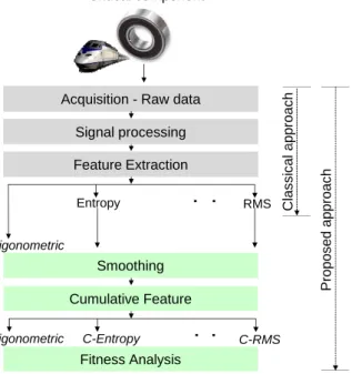
• The data-processing step is improved by introducing a new approach for features
extraction using trigonometric and cumulative functions, where features selection is based on three characteristics, i.e., monotonicity, trendability and predictability. The main idea of this development is to transform raw data into features that improve accuracy of long-term predictions.
• To account for robustness, reliability and applicability issues, a new prediction
algorithm is proposed: the Summation Wavelet-Extreme Learning Machine (SW-ELM). SW-ELM ensures good prediction performances while reducing the learning
improve accuracy of estimates.
• Prognostics performances are also enhanced thanks to the proposition of a new
health assessment algorithm: the Subtractive-Maximum Entropy Fuzzy Clustering (S-MEFC). S-MEFC is an unsupervised classification approach which uses max-imum entropy inference to represent uncertainty of unlabeled multidimensional data and can automatically determine the number of states (clusters), i.e., with-out human assumption.
• The final prognostics model is achieved by integrating SW-ELM and S-MEFC to
show evolution of machine degradation with simultaneous predictions and discrete state estimation. This scheme also enables to dynamically set failure thresholds and estimate RUL of monitored machinery.
Developments are validated on real data from three experimental platforms: PRONOS-TIA FEMTO-ST (bearings test-bed), CNC SIMTech (machining cutters), C-MAPSS NASA (turbofan engines) and other benchmark data. Due to realistic nature of the proposed RUL estimation strategy, quite promising results are achieved. However, reli-ability of the prognostics model still needs to be improved which is the main perspective of this work.
Acknowledgements
Special thanks to Almighty for the wisdom & perseverance, that he bestowed upon me throughout my Ph.D.
I am thankful to FEMTO-ST Institute & Universit´e de Franche-Comt´e Besan¸con (France) for the Ph.D. position & a unique research environment.
I would like to express my respect & gratitude to my supervisors Assoc. Prof. Rafael Gouriveau & Prof. Noureddine Zerhouni, for their continuous guidance, & valuable in-puts to my research.
I would like to thank my thesis reporters: Prof. Said Rechak, Prof. Enrico Zio, & the examiners: Prof. Louise Trav´e-Massuy`es, Prof. Antoine Grall, Prof. Janan Zay-toon for taking time to review my thesis.
I would like to acknowledge for the helpful suggestions from Assoc. Prof. Emmanuel Ramasso, Assoc. Prof. Kamal Medjaher & Dr. Tarak Benkedjouh. I also want to thank my other colleagues, without particular order: Syed Zill-e-Hussnain, Bilal Komati, Bap-tiste Veron, Nathalie Herr, Ahmed Mosallam, Haithem Skima & many others for the friendly environment & fruitful discussions.
Many thanks to my wife Momna for her support, & my little angel Musa who never let me go bored of my work.
I am grateful to my parents, my uncle, my brothers & other family members who sup-ported me over the years.
Finally, I won’t forget my friend Salik, who encouraged me to pursue my research career with this opportunity.
Kamran Javed
Contents
Acronyms & Notations xix
General introduction 1
1 Enhancing data-driven prognostics 5
1.1 Prognostics and Health Management (PHM) . . . 5
1.1.1 PHM as an enabling discipline . . . 5
1.1.2 Prognostics and the Remaining Useful Life . . . 8
1.1.3 Prognostics and uncertainty . . . 9
1.2 Prognostics approaches. . . 12
1.2.1 Physics based prognostics . . . 12
1.2.2 Data-driven prognostics . . . 13
1.2.3 Hybrid prognostics . . . 16
1.2.4 Synthesis and discussions . . . 19
1.3 Frame of data-driven prognostics . . . 22
1.3.1 Data acquisition . . . 22
1.3.2 Data pre-processing . . . 23
1.3.3 Prognostics modeling strategies for RUL estimation . . . 23
1.4 Open issues & problem statement for the thesis . . . 25
1.4.1 Defining challenges of prognostics modeling . . . 25
1.4.2 Toward enhanced data-driven prognostics . . . 27
1.5 Summary . . . 30
2 From raw data to suitable features 31 2.1 Problem addressed . . . 31
2.1.1 Importance of features for prognostics . . . 31
2.1.2 Toward monotonic, trendable and predictable features . . . 33
2.2 Data processing . . . 34
2.2.1 Feature extraction approaches. . . 34
2.2.2 Feature selection approaches . . . 36
2.3 Proposition of a new data pre-treatment procedure . . . 36 vii
2.3.2 Steps for feature extraction / selection . . . 38
2.4 First PHM case study on real data . . . 43
2.4.1 Bearings datasets of IEEE PHM Challenge 2012 . . . 43
2.4.2 Feature extraction and selection results . . . 44
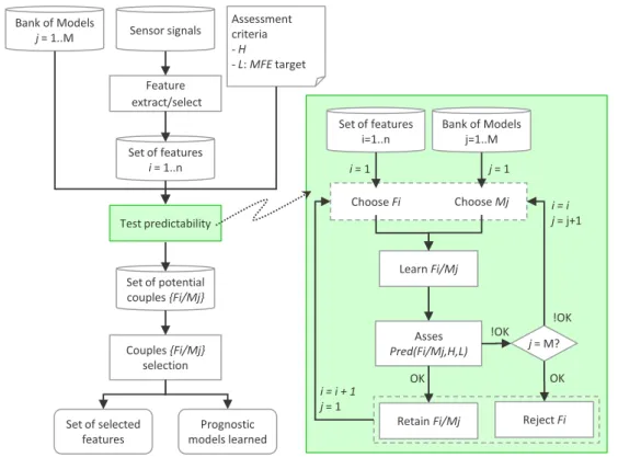
2.5 Predictability based prognostics: underlying concepts. . . 49
2.5.1 Proposition of a new data post-treatment procedure . . . 49
2.5.2 Predictability based feature selection procedure . . . 51
2.6 Second PHM case study on real data . . . 52
2.6.1 Outline . . . 52
2.6.2 Building a prognostics model . . . 54
2.6.3 Prognostics results and impact of predictability . . . 60
2.6.4 Observations . . . 62
2.7 Summary . . . 62
3 From features to predictions 65 3.1 Long-term predictions for prognostics . . . 65
3.2 ELM as a potential prediction tool . . . 67
3.2.1 From ANN to ELM . . . 67
3.2.2 ELM for SLFN: learning principle and mathematical perspective 68 3.2.3 Discussions: ELM for prognostics. . . 70
3.3 SW-ELM and Ensemble models for prognostics . . . 71
3.3.1 Wavelet neural network . . . 71
3.3.2 Summation Wavelet-Extreme Learning Machine for SLFN . . . . 73
3.3.3 SW-ELM Ensemble for uncertainty estimation . . . 77
3.4 Benchmarking SW-ELM on time series issues . . . 78
3.4.1 Outline: aim of tests and performance evaluation . . . 78
3.4.2 First issue: approximation problems . . . 79
3.4.3 Second issue: one-step ahead prediction problems. . . 81
3.4.4 Third issue: multi-steps ahead prediction (msp) problems . . . . 83
3.5 PHM case studies on real data . . . 85
3.5.1 First case study: cutters datasets & simulation settings . . . 85
3.5.2 Second case study: bearings datasets of PHM Challenge 2012 . . 96
3.6 Summary . . . 98
4 From predictions to RUL estimates 99 4.1 Problem addressed: dynamic threshold assignment . . . 99
4.1.1 Failure threshold: univariate approach and limits . . . 99
4.1.2 Failure threshold: multivariate approach and limits . . . 100
4.1.3 Toward dynamic failure threshold. . . 101
4.2 Clustering for health assessment: outline & problems . . . 101
4.2.1 Categories of classification methods . . . 101
4.2.2 Clustering and discrete state estimation . . . 102
4.3 Discrete state estimation: the S-MEFC Algorithm . . . 104
4.3.1 Background . . . 104
4.3.2 S-MEFC for discrete state estimation . . . 108
4.4 Enhanced multivariate degradation based modeling . . . 110
4.4.1 Outline: dynamic FTs assignment procedure . . . 110
4.4.2 Off-line phase: learn predictors and classifiers . . . 111
4.4.3 On-line phase: simultaneous predictions & discrete estimation. . 112
4.5 PHM case study on real data . . . 113
4.5.1 Turbofan Engines datasets of IEEE PHM Challenge 2008 . . . . 113
4.5.2 Performance evaluation and simulation setting . . . 114
4.5.3 Prognostics results on complete test data . . . 115
4.5.4 Benefits of the proposed approach . . . 120
4.6 Summary . . . 120
5 Conclusion and future works 121 Bibliography 125 A Appendix A 145 A.1 Taxonomy of maintenance policies . . . 145
A.1.1 Corrective maintenance . . . 146
A.1.2 Preventive maintenance . . . 146
A.2 Relation between diagnostics and prognostics . . . 147
A.3 FCM algorithm . . . 149
A.4 Metrics for model accuracy . . . 149
A.5 Benchmark datasets . . . 150
A.5.1 Carnallite surge tank dataset . . . 150
A.5.2 Industrial dryer dataset . . . 152
A.5.3 Mechanical hair dryer dataset . . . 153
A.5.4 NN3 forecasting data. . . 153
List of Figures
1.1 PHM cycle (adapted from [119]) . . . 7
1.2 Illustration of prognostics and RUL estimates . . . 9
1.3 Component health evolution curves (adapted from [178]). . . 10
1.4 Uncertainty bands associated with RUL estimations (adapted from [191]) 11 1.5 Series approach for hybrid prognostics model (adapted from [71]) . . . . 16
1.6 Battery capacity predictions and new pdf of RUL [169]. . . 17
1.7 Parallel approach for hybrid prognostics model (adapted from [71]) . . . 18
1.8 Classification of prognostics approaches . . . 19
1.9 Prognostics approaches: applicability vs. performance . . . 22
1.10 Univariate degradation based modeling strategy. . . 24
1.11 Direct RUL prediction strategy . . . 24
1.12 Multivariate degradation based modeling strategy. . . 25
1.13 Illustration of challenge: robustness. . . 26
1.14 Illustration of challenge: reliability . . . 27
1.15 Thesis key points scheme - toward robust, reliable & applicable prognostics 29 2.1 From data to RUL . . . 32
2.2 Effects of features on prognostics . . . 33
2.3 Feature extraction approaches (adapted from [211]). . . 35
2.4 Proposed approach to obtain monotonic and trendable features . . . 37
2.5 WT and DWT . . . 38
2.6 Classical features extracted from a degraded bearing . . . 39
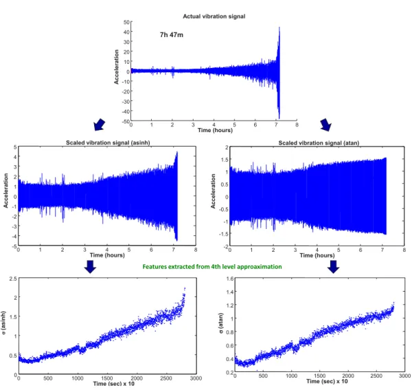
2.7 Trigonometric features extracted from a degraded bearing . . . 41
2.8 PRONOSTIA testbed - FEMTO-ST Institute, AS2M department. . . . 43
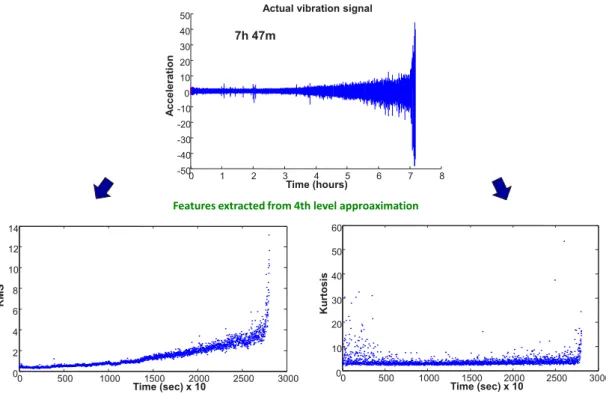
2.9 Bearing degradation: run-to-failure vibration signal. . . 44
2.10 Trigonometric features and classical features. . . 45
2.11 Extracted features and their respective cumulative features (good case) 46 2.12 Extracted features and their respective cumulative features (bad case) . 46 2.13 Fitness plots . . . 47
2.14 Comparison of classical and cumulative features on 17 bearings . . . 48
2.15 Compounds of predictability concept . . . 50 xi
2.17 Selection procedure based on predictability . . . 52
2.18 Engine diagram [72] . . . 53
2.19 Filtered feature from engine dataset . . . 53
2.20 Procedure to analyze the impact of predictability . . . 54
2.21 Iterative model for multi-steps predictions [76] . . . 55
2.22 Predictability of features forH =tc+ 134 . . . 57
2.23 Example of degrading feature prediction . . . 58
2.24 Visualization of classes from multidimensional data of 40 engines . . . . 60
2.25 ED results (test−1): a),b) All features and c),d) Predictable features . 60 2.26 Classification with all features. . . 61
2.27 Classification with predictable features . . . 61
3.1 Discrete state estmation and RUL estimation [76]. . . 67
3.2 Structure of FFNN and RNN [102] . . . 68
3.3 Single layer feed forward neural network . . . 69
3.4 Mother and daughter wavelet from Morlet function . . . 72
3.5 Structure and learning view of proposed SW-ELM . . . 75
3.6 SW-ELME and confidence limit interval (CI) . . . 78
3.7 Fault code approximations and corresponding errors . . . 80
3.8 Tool wear estimation and corresponding errors . . . 81
3.9 One-step ahead prediction of bulb temperature and corresponding errors 82 3.10 One-step ahead prediction of Air temperature and corresponding errors 82 3.11 msp of time series 61 (NN3) . . . 84
3.12 msp of sensor 2 (Engine 5) . . . 84
3.13 Accuracy of: a)msp for 8 NN3 series, b)msp for 5 Turbofan engines. . 84
3.14 Cutting force signals in three axes (Fx, Fy, Fz) [223] . . . 85
3.15 Cutting tool wear estimation - methodology . . . 87
3.16 Force features extracted from 315 cuts . . . 87
3.17 Robustness: learning and testing with one cutter . . . 88
3.18 Robustness analysis: partially unknown data for a “single cutter” model 89 3.19 Reliability: learning and testing with three cutters . . . 90
3.20 Reliability analysis: partially unknown data for “multi-cutter” model. . 91
3.21 Reliability: learning and testing with unknown data . . . 92
3.22 Reliability analysis with totally unknown data. . . 93
3.23 Estimation with multi-cutter model on unknown data . . . 93
3.24 Tool wear evolution and precise wear limit . . . 95
3.25 Cutting tools wear estimation and CI construction . . . 96
3.26 Examples of multi-step ahead predictions (Classical vs. Proposed) . . . 98
4.1 Transition from healthy to degrading state [75] . . . 101
4.2 Usefulness and limits of classification methods in PHM (adapted from [75])102 4.3 Discrete state estimation from multidimensional data . . . 103
4.5 Density measurement for each data point [4]. . . 107
4.6 Revised density measuring procedure [4] . . . 108
4.7 Example of clustering withDSE (left) and ED (right) metrics [3] . . . . 109
4.8 Enhanced multivariate degradation based modeling strategy . . . 111
4.9 off-line phase . . . 112
4.10 Simultaneous predictions and state estimation . . . 113
4.11 Sensor measurement from 100 engines (training data) and life spans . . 113
4.12 Prediction interval [166] . . . 114
4.13 RUL estimation - Test 1 . . . 115
4.14 Visualization of classes and data point membership functions . . . 116
4.15 Dynamic threshold assignment results (for discrete states) . . . 117
4.16 Actual RUL vs. estimated RUL (100 Tests) . . . 118
4.17 RUL error distribution a) proposed approach and b) by [166] . . . 119
4.18 Scores for 100 tests (enhanced multivariate degradation based modeling) 119 A.1 Classification of maintenance policies in industry . . . 145
A.2 Steps to obtain prognostics results & relationship to diagnostics [178]. . 148
A.3 Input data: RMS and variance . . . 151
A.4 Output targets . . . 151
A.5 Input data. . . 152
A.6 Output: dry bulb temperature . . . 152
A.7 Voltage of heading device and air temperature . . . 153
List of Tables
1.1 7 layers of PHM cycle . . . 7
1.2 Prognostics approach selection . . . 22
2.1 Features extracted from 4th level Approximation . . . 40
2.2 Datasets of IEEE PHM 2012 Prognostics challenge . . . 44
2.3 Features fitness analysis . . . 47
2.4 Comparing features fitness (mean performances on 17 bearings) . . . 48
2.5 C-MPASS output features . . . 53
2.6 Prediction models - Settings . . . 56
2.7 Predictability results on a single test . . . 57
2.8 RUL percentage error with ANFIS . . . 62
3.1 Datasets to benchmark performances for time series application . . . 79
3.2 Approximation problems: results comparison . . . 80
3.3 One step-ahead prediction problems: results comparison . . . 82
3.4 Multi-setp ahead prediction problems: results comparison . . . 84
3.5 Type of cutting tools used during experiments. . . 86
3.6 Robustness and applicability for a single cutter model . . . 89
3.7 Reliability and applicability for 3 cutters models . . . 90
3.8 Reliability and applicability for unknown data. . . 92
3.9 Tool wear estimation with SW-ELME - Settings . . . 94
3.10 Reliability and applicability for unknown data with SW-ELME . . . 95
3.11 Long term prediction results for 5 test bearings . . . 97
4.1 Prognostics model results comparison for 100 test engines . . . 117
List of Algorithms
1 Learning scheme of an ELM . . . 70
2 Learning scheme of the SW-ELM . . . 76
3 S-MEFC . . . 110
4 Key steps of FCM algorithm . . . 149
Acronyms & Notations
ANFIS Adaptive Neuro-Fuzzy Inference System
ANN Artificial Neural Networks
CBM Condition Based Maintenance
CI Confidence Intervals
CM Condition Monitoring
CNC Computer Numerical Control machine
CV RM SE Coefficient of Variation of the Root Mean Square Error
CWT Continuous Wavelet Transform
DD Data-driven approach
DWT Discrete Wavelet Transform
DSE Standardized Euclidean Distance
ED Euclidean Distance
ELM Extreme Learning Machine
EOL End Of Life
FCM Fuzzy C-Means
FFNN Feed Forward Neural Network
FT Failure Threshold
Hyb Hybrid approach
M Models of prediction
M AP E Mean Average Percent Error
MEFC Maximum Entropy based Fuzzy Clustering
MEI Maximum entropy inference
M F E Mean Forecast Error
MRA Multi-Resolution Analysis
msp Multi-steps ahead predictions
NFS Neuro-Fuzzy System
NW Nguyen Widrow procedure
PHM Prognostics and Health Management
POF Physics of failure
RMS Root Mean Square
RUL Remaining Useful Life
SC Subtractive Clustering
SLFN Single Layer Feed Forward Neural Network
SW-ELM Summation Wavelet-Extreme Learning Machine
SW-ELME Summation Wavelet-Extreme Learning Machine Ensemble
S-MEFC Subtractive-Maximum Entropy Fuzzy Clustering
WT Wavelet transform
b Hidden node bias (i.e., SLFN)
c Number of clusters
C Constant
CF´ Cumulative Feature
d Dilate (or scale) daughter wavelet
f Activation function for hidden nodes
¯
f Average output from two different activation functions
F or ´F Feature
H Hidden layer output matrix
H† Moore-Penrose generalized inverse
Havg Average of two hidden layer output matrix
ℓD Learning data for prognostics model
¨
M Monotonicity
˜
N Number of hidden nodes
ˆ
om
j Predicted output ofmth model against the jth input sample
o Prediction model output (i.e., SLFN)
O Averaged output from multiple prediction models
R2 Coefficient of determination
s Translate (or shifts) daughter wavelet
t Outputs samples
tc Current time
tD Time of degradation
tf Time at which prediction passes the FT
U Fuzzy partition matrix
v Cluster center
V Cluster centers matrix
w Input-hidden neuron weights
x Inputs samples
β Output weight matrix
Ψ Mother wavelet
µij Membership of theith data point to thejth centroid
σo2j Variance
General introduction
Any machine during its service life is prone to degrade with the passage of time. How-ever, the failure of engineering assets or their critical machinery can not only be a loss in the manufacturing process or timely services to the customers, but can also have major negative outcomes. In some cases, machinery malfunctioning can even result in irreversible damages to the environment or in safety problems, for example, jet crash due to engine failure, rail accident due to bearing failure, etc. This highlights the need to maintain critical machinery before a failure could happen.
Generally, maintenance can be defined as, “the combination of all technical and associ-ated administrative actions intended to retain a system in a state at which it can perform
the required function” [66]. With recent advances in modern technology, industrials and
researchers are progressing toward enhanced maintenance support systems that aim at improving reliability and availability of critical engineering assets while reducing over-all costs. Therefore, the role of maintenance has changed from a “necessary evil” to a
“profit contributor” [194]. Also, the trends have grown rapidly and shifted from fail-fix
maintenance to predict-prevent maintenance. In this context, one should speak about
the evolution in maintenance policies [66], that began from unplanned corrective
main-tenance practices for non-critical machinery, and then shifted to a planned preventive maintenance (PM). More precisely, the PM is performed by either pre-defined schedule or by performing Condition-Based Maintenance (CBM) on the basis of current state of the machinery. Further, the CBM evolved to predictive maintenance strategy, that is based on forecasts of future evolution of machine degradation. Therefore, upon
de-tection of failure precursors, prognostics 1 becomes a necessary step to anticipate (and
predict) the failure of degrading equipment at future times to estimate the Remaining
Useful Life (RUL) [226]. Indeed, it is assumed that adequate actions (either maintenance
tasks, either load profile changes) must be performed in a timely manner, such that, crit-ical failures that could lead to major breakdowns or huge wastes can be avoided, which enables optimizing machinery service delivery potential during its lifetime. To fulfill such time critical needs, an enhanced application of CBM is through prognostics, and therefore, CBM has evolved into the concept of Prognostics and Health Management.
1Note: In literature keywords prognosis, prognostic or prognostics are used, but for the thesis the word “prognostics” is considered.
For modern industry, PHM appears to be a key enabler for improving availability of crit-ical engineering assets while reducing inopportune spending and security risks. Within the framework of PHM, prognostics is considered as a core process for deploying an effective predictive maintenance scheme. Prognostics is also called as the “prediction of a system’s lifetime”, as its primary objective is to intelligently use the monitoring information of an in-service machinery, and to predict its RUL before a failure occurs,
given the current machine condition and its past operation profile [105].
Machinery operates in a dynamic environment, where its behavior is often non-linear due to different factors like environmental and operating conditions, temperature, pressure, noise, engineering variance, etc. As a result, the condition monitoring data gathered from machinery are subject to high levels of uncertainty and unpredictability. Also, with lack of knowledge and understanding about complex deterioration processes, pre-dicting behavior of an in-service machinery can be a complicated challenge. Although in the past decade there are several efforts around the world, real prognostics systems to meet industrial challenges are still scarce. This can be due to a highly complex and non-linear operational environment of industrial systems, which makes it hard to establish effective prognostics approaches that are: robust enough to tolerate uncertainty, reliable enough to show acceptable performance under diverse conditions, and applicable enough to fit industrial constraints. As a result, the need for an enhanced prognostics approach can be pointed out.
In this thesis, the developments are achieved following a thorough literature review on three different approaches for prognostics, i.e., physics based, data-driven, and hybrid approaches. This enables identifying the key challenges related to implementation of a prognostics model, i.e., robustness, reliability and applicability. To account for such challenges, a novel approach for prognostics is introduced by applying advanced tech-niques from data-driven category of prognostics approaches. The overall performances of data-driven prognostics framework are enhanced by focusing on data-processing, health assessment, and behavior prediction steps. Most importantly, as compared to conven-tional approaches of data-driven prognostics, RUL estimation is achieved by integrating two newly developed rapid machine learning algorithms. The proposed developments also give a new direction to perform prognostics with a data-driven approach.
The structure of the thesis manuscript is organized as follows.
Chapter 1 gives an overview of PHM, and the role of prognostics. Following that a thorough survey on the classification of prognostics approaches is presented including their pros and cons. Different RUL estimation strategies with data-driven approaches are also reviewed, and the challenges of prognostics modeling are defined.
Chapter 2discusses the importance of data-processing, its impact on prognostics mod-eling, and on the accuracy of RUL estimates. Therefore, developments are focused on features extraction and selection steps, and aim at obtaining features that clearly reflect machine degradation, and can be easily predicted. In order, to validate the propositions, two PHM case studies are considered: real data of turbofan engines from PHM challenge
Introduction 3 2008, and real data of bearings from PHM challenge 2012.
Chapter 3 presents a new rapid learning algorithm, the Summation Wavelet-Extreme Learning Machine (SW-ELM) that enables performing “long-term predictions”. For issues related to time series (i.e., approximation, one step-ahead prediction, multi-step ahead prediction) and challenges of prognostics modeling, the performances of SW-ELM are benchmarked with different approaches to show its improvements. An ensemble of SW-ELM is also proposed to quantify uncertainty of the data / modeling phase, and to improve accuracy of estimates. In order, to further validate the proposed prediction algorithm, two PHM case studies are considered: real data of a CNC machine, and real data of bearings from PHM challenge 2012.
Chapter 4 is dedicated to the complete implementation of prognostics model, and its validation. Firstly, a new unsupervised classification algorithm is proposed namely, the Subtractive-Maximum Entropy Fuzzy Clustering (S-MEFC), that enables estimat-ing the health state of the system. Secondly, a novel strategy for RUL estimation is presented by integrating SW-ELM and S-MEFC as a prognostics model. The proposed approach allows tracking the evolution of machine degradation, with simultaneous pre-dictions and discrete state estimation and can dynamically set the failure thresholds. Lastly, to investigate the efficiency of the proposed prognostics approach, a case study on the real data of turbofan engines from PHM challenge 2008 is presented, and the comparison with results from recent publications is also given.
Chapter 5 concludes this research work by summarizing the developments, improve-ments and limitations. A discussion on the future perspectives is also laid out.
Chapter
1
Enhancing data-driven prognostics
This chapter presents a thorough survey on Prognostics and Health Manage-ment literature, importance of prognostics, its issues and uncertainty. Also, a detailed classification of prognostics approaches is presented. All categories of prognostics approaches are assessed upon different criteria to point out their importance. Thereby, recent strategies of RUL estimation are reviewed and the challenges of prognostics modeling are defined. Thanks to that, the problem statement and objectives of this thesis are finally given at the end of the chapter.
1.1
Prognostics and Health Management (PHM)
1.1.1 PHM as an enabling discipline
With aging, machinery or its components are more vulnerable to failures. Availability and maintainability of such machinery are of great concern to ensure smooth functioning and to avoid unwanted situations. Also, the optimization of service and the minimiza-tion of life cycle costs / risks require continuous monitoring of deterioraminimiza-tion process, and reliable prediction of life time at which machinery will be unable to perform
de-sired functionality. According to [87], for such requirements, the barriers of traditional
Condition-Based Maintenance (CBM) for widespread application, identified during a 2002 workshop organized by National Institute of Standards and Technology (USA), are as follows:
1. inability to continually monitor a machine;
3. inability of maintenance systems to learn and identify impending failures and recommend what action should be taken.
These barriers can be further redefined as deficiencies in sensing, prognostics and rea-soning. Also, over the last decade, CBM has evolved into the concept of Prognostics and
Health Management (PHM) [87], due to its broader scope. Basically, PHM is an
emerg-ing engineeremerg-ing discipline which links studies of failure mechanisms (corrosion, fatigue,
overload, etc.) and life cycle management [191]. It aims at extending service cycle of an
engineering asset, while reducing exploitation and maintenance costs. Mainly, acronym
PHM consists of two elements [85,87,226].
1. Prognostics refers to a prediction / forecasting / extrapolation process by mod-eling fault progression, based on current state assessment and future operating conditions;
2. Health Management refers to a decision making capability to intelligently per-form maintenance and logistics activities on the basis of diagnostics / prognostics information.
PHM has by and large been accepted by the engineering systems community in general,
and the aerospace industry in particular, as the future direction [172]. Among different
strategies of maintenance (AppendixA.1), PHM is contemporary maintenance strategy
that can facilitate equipment vendors, integrators or operators to dynamically maintain
their critical engineering assets. According to [191], in U.S military two significant
weapon platforms were designed with a prognostics capability: Joint Strike Fighter
Program [85], and the Future Combat Systems Program [22]. As technology is maturing,
PHM is also and active research at NASA for their launch vehicles and spacecrafts [149].
In other words, PHM is a key enabler to facilitate different industries to meet their desired goals e.g. process industry, power energy, manufacturing, aviation, automotive, defence, etc. Some of the key benefits of PHM can be highlighted as follows:
• increase availability and reduce operational costs to optimized maintenance;
• improve system safety (predict to prevent negative outcomes);
• improve decision making to prolong life time of a machinery.
PHM makes use of past, present and future information of an equipment in order to
assess its degradation, diagnose faults, predict and manage its failures [226]. Considering
such activities, PHM is usually described as the combination of 7 layers adapted from
Open System Architecture for CBM [119,140], that all together enable linking failure
mechanisms with life management (Fig. 1.1). We can divided these layers into three
1.1 Prognostics and Health Management (PHM) 7
Table 1.1: 7 layers of PHM cycle
Observe 1.Data acquisition: gather useful condition monitoring (CM) data records using
digitized sensors.
2.Data processing: perform data cleaning, denoising, relevant features extraction and selection.
Analyze
3.Condition assessment: assess current condition of monitored machinery, and degradation level.
4.Daignostics: perform diagnostics to detect, isolate and identify faults (see AppendixA.2).
5.Prognostics: perform prognostics to project current health of degrading mach-inery onto future to estimate RUL and associate a confidence interval.
Act 6.Decision support: (off-line) recommend actions for maintenance / logistic
(e.g. service quality), and (on-line) system configuration (safety actions). 7.Human Machine Interface: interact with different layers, e.g. prognostics,
decision support and display warnings etc.
641 641.5 642 642.5 643 643.5 644 2387.9 2387.95 2388 2388.05 2388.1 2388.15 2388.2 2388.25 2388.3 2388.35 0 2000 4000 6000 8000 10000 12000 12 13 14 U ( V ) 0 1000 200030004000 50006000 17 18 19 20 N iv e a u 1 0 100020003000400050006000 -0.1 0 0.1 Temps (min) PHM Condition Assessment Diagnostic Prognostics Data Acquisition Data Processing Decision Support Human Machine Interface
Figure1.1: PHM cycle (adapted from [119])
Within analysis phase, prognostics is considered as a key task with future capabilities, which should be performed efficiently for successful decision support to recommend
actions for maintenance [13], or system configuration [14]. Therefore, prognostics is a
core process in PHM cycle, to decide plan of actions, increase safety, minimize downtime,
1.1.2 Prognostics and the Remaining Useful Life
The concept of prognostics was initially introduced in the medical domain. Medical prognostics is defined as “the prediction of the future course and the outcome of disease
process” [8]. In engineering, prognostics is generally understood as the process of
moni-toring health of an engineering asset, and of predicting the life time at which it will not perform the required function. According to literature, there are several definitions of
prognostics [178], but, few interesting ones are given as follows:
1. the capability to provide early detecting of the precursor and / or incipient fault condition of a component, and to have the technology and means to manage and
predict the progression of this fault condition to component failure [67];
2. predictive diagnostics, which includes determining the remaining life or time span
of proper operation of a component [86];
3. the prediction of future health states based on current health assessment, historical
trends and projected usage loads on the equipment and / or process [207];
4. failure prognostics involves forecasting of system degradation based on observed
system condition [133];
5. the forecast of an asset’s remaining operational life, future condition, or risk to
completion [83].
A common acceptance can be dressed from above definitions: prognostics can be seen as the “prediction of a system’s lifetime” as it is a process whose objective is to predict the Remaining Useful Life before a failure occurs. Also, let retain the definition proposed
by the International Organization for Standardization [99]:
“prognostics is the estimation of time to failure and risk for one or more existing and future failure modes”.
Note that, the implementation of prognostics for a particular application can be made at different levels of abstraction like: critical components, sub-system or entire system. Also, RUL is expressed by considering units corresponding to the primary measurement of use for overall system. For example, in case of commercial aircrafts the unit is cycles (i.e., related to number of take-offs), for aircraft engines it is hours of operation, for au-tomobiles it is kilometers (or miles). Having said that, whatever the level of abstraction and the unit to define that, prognostics facilitate decision makers with information, that enables them to change operating conditions (e.g. load). Consequently, it may prolong service life of the machinery. In addition, it also benefits the planners to manage up-coming maintenance and to initiate a logistics process, that enables a smooth transition
from faulty machinery to fully functional [175].
The main capability of prognostics is to help maintenance staff with insight of future health states of a monitored system. This task is mainly composed of two different steps. The first step is related to the assessment of current health state (i.e., severity or degradation detection), which can also be considered under detection and diagnostics.
1.1 Prognostics and Health Management (PHM) 9 Different pattern recognition techniques can be applied to this phase. The second step aims at predicting (or forecasting) degradation trends to estimate the RUL, where time
series techniques can be applied [63].
As for illustration of RUL estimation task, consider left part of Fig.1.2, where for sake
of simplicity the degradation is considered as a one-dimensional signal. In such case,
the RUL can be computed between current time tcafter degradation has been detected
tD, and the time at which predicted signal passes the failure threshold (FT) (assumed
or precisely set by an expert), i.e., timetf, with some confidence to the prediction. The
FT does not necessarily indicate complete failure of the machinery, but a faulty state
beyond which there is a risk of functionality loss [171], and end of life (EOL). Therefore,
RUL can be defined by Eq. (1.1):
RU L=tf−tc (1.1)
where tf is a random variable of time to failure, andtcis the current time.
Degradation detected Time (t) R U L Actual RUL EOL Estimated RUL &
confidence
Time (t)
Estimated RUL
tD tc
(end of life - EOL) Complete Failure Failure threshold (FT) D eg rad in g s ta te U nc er tai n (F T ) tf tc Actual RUL
Figure 1.2: Illustration of prognostics and RUL estimates
Providing a confidence to predictions is essential for prognostics due to inherent un-certainties of deterioration phenomena, unclear future operating conditions and errors associated to the prognostics model. Therefore, decision making should be based on
the bounds of RUL confidence interval rather than single value [178]. Also, narrow
confidence intervals represent high precision / accuracy and are preferred over wide con-fidence intervals that indicate large uncertainty, thus risky decisions should be avoided. Therefore, the combined uncertainty of RUL estimate is not only due to prediction but due to the FT as well (which should be precise).
The right part of Fig.1.2shows a situation, where estimated RUL value is updated when
new data arrives at each time interval. In this manner, different RULs are estimated with some confidence according to availability of data from monitored machinery. Obviously, accuracy of RUL estimates should increase with time, as more data are available.
1.1.3 Prognostics and uncertainty
Aging of machinery in a dynamic environment is a complex phenomena, and it is often
real monitoring data from machinery condition (vibration, temperature, humidity, pres-sure, etc.,) are usually noisy and open to high variability due to direct or indirect impact of usage and environmental conditions related to the degradation of failing machinery. In other words, real-life machinery prognostics is subject to high levels of uncertainty, either due to gathered data or either due to degradation mechanisms. As for example, consider a process, where a component degrades from a healthy state to failure state
(see Fig.1.3). The same component can have different degrading curves due to different
failure modes (e.g. in case of bearings inner race, outer race, cage crack), even exposed to same operating conditions. Although, failure modes can be for a same bearing, but still each mode can result different states of degradation that result different RULs. In such situations, RUL estimation becomes a complicated challenge for the prognostics model, that requires timely predicting the future unknown and intelligently assessing the faulty state.
Novel event
Novel event
Degraded but operable state
Functional failure Failure mode 1 Failure mode 2 Failure mode 3 C o m p o n e n t H e a lt h Time Bearing Inner race Balls in cage Outer race
Figure1.3: Component health evolution curves (adapted from [178])
From the above discussions, some key issues of prognostics can be pointed out.
• How to tackle inherent uncertainties of data?
• How to represent uncertainty of machine deterioration process (i.e., from good to
faulty state)?
• How to avoid uncertainty of FTs, to enable accurate RUL estimates?
Such issues can be related to different sources of uncertainty [40].
1. Input uncertainties that can be due to initial damage, material properties, manu-facturing variability, etc.
1.1 Prognostics and Health Management (PHM) 11 2. Model uncertainties that can be due to modeling error related to inaccurate pre-dictions (for data-driven prognostic approaches it can be related to incomplete
coverage of data model training [71]). However, such uncertainties can be reduced
by improved modeling methods.
3. Measurement uncertainties that are related to data collection, data processing, etc., and can be managed to a better level. For example sensor noise, loss of information due to data processing, etc.
4. Operating environment uncertainties like unforeseen future loads or environments. Whatever the type of uncertainties in prognostics, they can impact the accuracy of RUL estimates which prevents to recommend timely actions for decision making process or system configuration. In brief, for prognostics system development, three different
processes are essential to handle uncertainty [40].
• To represent uncertainty of data, which include common theories like fuzzy set
theory, probability theory, etc.;
• To quantify uncertainty related to different sources as correctly as possible;
• To manage the uncertainty by processing the data in an effective manner.
For example consider situation in Fig. 1.4, that illustrates the uncertainty of the RUL
estimation by a prognostics model and updates its predictions when new data arrives. Initially the equipment is new and accumulated damage is minor, therefore uncertainty regarding the unknown future can be high. When the damage grows and the failure point is closer, the prognostics model can have much less uncertainty to estimate the exact time to failure. In addition, it is necessary to account for different sources of uncertainties of prognostics, that are associated with “long-term predictions” of machinery health. Without such information a prognostics model has limited use and cannot be integrated
Failure Threshold (FT) D e g ra d a tion Time/cycles P1 P2 P3 updated prediction at P2 updated prediction at P3
for critical applications. Therefore, in this thesis, uncertainty of prognostics is dealt by: quantifying uncertainty due to data and modeling phase, representing uncertainty using fuzzy set theory, and managing uncertainty by processing data.
1.2
Prognostics approaches
The core process of prognostics is to estimate the RUL of machinery by predicting the future evolution at an early stages of degradation. An accurate RUL estimation enables to run the equipment safely as long as it is healthy, which benefits in terms of additional time to opportunely plan and prepare maintenance interventions for most convenient
and inexpensive times [105]. Due to the significance of such aspects, study on PHM
has grown rapidly in recent years, where different prognostics approaches are being developed. Several review papers on the classification of prognostics approaches have
been published [60,74,105,115,153,156,177,178,192,193]. In spite of divergence in
literature, we bring discussions on common grounds, where prognostics approaches are classified into three types: 1) physics based prognostics, 2) data-driven prognostics and 3) hybrid prognostics. But still, these classes are not well addressed in literature, which requires a detailed survey.
1.2.1 Physics based prognostics
1.2.1.1 Overview
The physics based or model based approaches for prognostics use explicit mathematical representation (or white-box model) to formalize physical understanding of a degrading
system [155]. RUL estimates with such approaches are achieved on the basis of acquired
knowledge of the process that affects normal machine operation and can cause failure. They are based on the principle that failure occurs from fundamental processes:
me-chanical, electrical, chemical, thermal, radiation [154]. Common approaches of physics
based modeling include material level models like spall progression models, crack-growth
models or gas path models for turbine engines [84,178,191]. To identify potential failure
mechanisms, such methods utilize knowledge like loading conditions, geometry, and
ma-terial properties of a system [153]. To predict the behavior of the system, such methods
require detailed knowledge and through understanding of the process and mechanisms that cause failure. In other words, failure criteria are created by using physics of failure
(POF) analysis and historic data information about failed equipment [88].
Implementa-tion of physics based approach has to go through number of steps that include, failure
modes and effects analysis (FMEA), feature extraction, and RUL estimation [153].
It should be noted that in literature, different works categorize physics based (or
model-based) prognostics as POF and system modeling approach [155, 158]. However, they
should be limited to POF [192, 197], because system modeling approaches are
depen-dent on data-driven methods to tune parameters of physics based model and should be
1.2 Prognostics approaches 13
1.2.1.2 Application point of view
In general, physics based approaches are application specific. They assume that sys-tem behavior can be described analytically and accurately. Physics based methods are suitable for a situation where accuracy outweighs other factors, such as the case of air
vehicles [168]. POF models are usually applied at component or material level [197].
However, for most industrial applications physics based methods might not be a proper choice, because fault types can vary from one component to another and are difficult
to identify without interrupting operating machinery [84]. In addition, system
spe-cific knowledge like material composition, geometry may not be always available [155].
Besides that, future loading conditions also affect fault propagation. Therefore in a dynamic operating environment, the model may not be accurate due to assumptions,
errors and uncertainty in the application [197]. In such cases POF models are combined
with data-driven methods to update model parameters in an on-line manner, which
turns into a hybrid approach (and is discussed in section 1.2.3).
1.2.2 Data-driven prognostics
Data-driven (DD) prognostics approaches can be seen as black box models that learn systems behavior directly from collected condition monitoring (CM) data (e.g. vibration, acoustic signal, force, pressure, temperature, current, voltage, etc). They rely on the assumption that the statistical characteristics of system data are relatively unchanged unless a malfunctioning occurs. Such methods transform raw monitoring data into rel-evant information and behavioral models (including the degradation) of the system. Therefore, data-driven methods can be low cost models with an advantage of better
applicability, as they only require data instead of prior knowledge or human experts
[110,111,155].
According to literature, several studies are performed to categorize data-driven
prog-nostics approaches. [63, 220] classified data-driven methods into machine learning and
statistical approaches. [60,156] classified data-driven approaches as artificial intelligence
(AI) techniques and Statistical techniques. A survey on AI approaches for prognostics
was presented by [176], where data-driven approaches were categorized as conventional
numerical methods and machine learning methods. [158] classified data-driven
prognos-tics methods as, evolutionary, machine learning / AI and state estimation techniques. However, we classify data-driven approaches for prognostics into two categories. 1) machine learning approaches and 2) statistical approaches.
1.2.2.1 Machine learning approaches
Machine learning approaches are branch of AI that attempt to learn by examples and are capable to capture complex relationships among collected data that are hard to describe. Obviously, such methods are suitable for situations where physics based modeling are
not favorable to replicate behavior model [111]. Depending on the type of available
to labeled data, i.e., data are composed of input and the desired output is known. Un-supervised learning is applied to unlabeled data, i.e., learning data are only composed of input and desired output is unknown. Semi-supervised learning that involves both labeled (few data points) and unlabeled data. A partially supervised learning is per-formed when data have imprecise and / or uncertain soft labels, (i.e., learning data are
composed of input and desired outputs are known with soft labels or belief mass [50]).
Machine learning is a rapidly growing field in PHM domain, and vast numbers of algo-rithms are being developed. In brief, machine learning approaches for prognostics can be categorized with some examples as follows.
Connectionist methods - Flexible methods that use examples to learn and infer complex relations among data e.g.:
• Artificial neural networks (ANN) [9,107,134];
• Combination of ANN and Fuzzy rules, e.g. Neuro-Fuzzy systems [59,107].
Bayesian methods - Probabilistic graphical methods mostly used in presence of uncertainty, particularly dynamic Bayesian approaches e.g.:
• Markov Models and variants, e.g. Hidden Markov Models (HMM) [138,165];
• State estimation approaches, e.g. Kalman Filter, Particle Filter and variants [20,
174,178].
Instance Based Learning methods (IBL) - Obtain knowledge from stored ex-amples that were presented for learning and utilize this knowledge to find similarity between learned examples and new objects:
• K-nearest neighbor algorithm [142];
• Case-based reasoning for advanced IBL [197].
Combination methods - Can be an effective combination of supervised, unsuper-vised methods, semi-superunsuper-vised and partially superunsuper-vised methods or other possible com-binations to overcome drawbacks of an individual data-driven approach, for e.g.:
• Connectionist approach and state estimation techniques [18];
• Connectionist approach and clustering methods [108,164];
• Ensemble of different approaches to quantify uncertainty and to achieve robust
models [17,20,89].
Note that, some of the above mentioned categories can also include supervised, unsu-pervised, semi-supervised learning or partially supervised approaches, however we avoid any strict classification.
1.2 Prognostics approaches 15
1.2.2.2 Statistical approaches
They estimate the RUL by fitting the probabilistic model to the collected data and ex-trapolate the fitted curve to failure criteria. Statistical approaches are simple to conduct. Like machine learning approaches, statistical methods also require sufficient condition monitoring (CM) data to learn behavior of degrading machinery. However, they can have large errors in case of incomplete data, and the nature of data has therefore its own importance in this category.
[177] presented a state-of-the-art review of statistical approaches, where the taxonomy
was mainly based on nature of CM data. From this systematic review, some commonly known prognostics approaches can be: regression based methods, stochastic filtering or state estimation methods like Kalman Filters Particle Filters and variants, Hidden Markov models and variants etc. Further details about this taxonomy are described
in [177]. It should be noted that, Bayesian techniques cited just above can also be
addressed as machine learning approaches. Other methods in this category can be clas-sical time series prediction methods like Auto-Regressive Moving Average and variants
or proportional hazards models [178].
1.2.2.3 Application point of view
In general, the strength of data-driven approaches is their ability to transform
high-dimensional noisy data into low-high-dimensional information for prognostics decisions [60].
However, data-driven methods encounter common criticism that they require more data as compared to physics based approach, which is not surprising. Obviously sufficient quantities of run-to-failure data are necessary for data-driven models to learn and cap-ture complex relations among data. In this context, sufficient quantity means that data
has been observed for all fault-modes of interest [191]. However, some industrial systems
can not be allowed to run until failure due to their consequences.
Beside that, quantity and quality of data are also important. Indeed, real machinery op-erates in highly non-linear environment and monitored data could be of high variability, sensor noise, which can impact on performance of data-driven methods. Therefore, it is essential to properly process acquired data in order to obtain good features to reduce modeling complexity, and increase accuracy of RUL estimates.
Machine learning approaches have the advantage that, they can be deployed rapidly and with low implementation cost as compared to physics based methods. In addition, they can provide system-wide scope, where scope of physics based approaches can be limited. Machine learning approach for prognostics could be performed with a connectionist feed
forward neural network [107] to predict continuous state of degradation recursively, until
it reaches FT. However, such methods provide point predictions and do not furnish any
confidence [111]. In comparison, Bayesian methods can be applied to manage
uncer-tainty of prognostics [40], but, again RUL estimates rely on FT. Instance based learning
methods do not need FT and can directly estimate the RUL by matching similarity
among stored examples and new test instances [142]. They can also be called as
can be a suitable choice to overcome drawbacks of an individual method [164]. But, whatever the approach considered for building a prognostics model, it is important to involve operating conditions and actual usage environment.
Lastly, statistical approaches for prognostics also require large amount of failure data to implement models. These approaches are economical and require fewer computations as compared to machine learning approaches. For e.g. methods like classical regression are simpler to build. However, they do not consider operating conditions, actual usage
environments and failure mechanism [220].
1.2.3 Hybrid prognostics
A hybrid (Hyb) approach is an integration of physics based and data-driven prognostics approaches, that attempts to leverage the strengths from both categories. The main idea is to benefit from both approaches to achieve finely tuned prognostics models that have better capability to manage uncertainty, and can result in more accurate RUL estimates.
According to literature, hybrid modeling can be performed in two ways [157]: 1) series
approach, and 2) parallel approach.
1.2.3.1 Series approach
In PHM discipline, series approach is also known as system modeling approach that
combines physics based approach havingprior knowledge about the process being
mod-eled, and a data-driven approach that serves as a state estimator of unmeasured process
parameters which are hard to model by first principles [160]. Several works in recent
literature address series approach as model based prognostics [19,155,158,174].
How-ever it cannot be regarded as model based, because, physics based model is dependant
on a data-driven approach to tune its parameters (see Fig.1.5).
Figure 1.5: Series approach for hybrid prognostics model (adapted from [71])
In brief, the representation (or modeling) of an engineering asset is made with mathe-matical functions or mappings, like differential equations. Statistical estimation methods based on residuals and parity relations (i.e., difference of predictions from a model and system observations) are applied to detect, isolate and predict degradation to estimate
1.2 Prognostics approaches 17 might be hard to achieve, where the state of the degrading machinery may not be
observ-able directly or measurements may be affected by noise [71]. In this case, a mathematical
model is integrated with on-line parameter estimation methods to infer degrading state and furnish reliable quantification of uncertainty. State estimation techniques can be
Bayesian methods like Kalman filter, Particle filter and variant [178], that update the
prediction upon collection of new data [57,58] (see Fig.1.6).
Figure 1.6: Battery capacity predictions and new pdf of RUL [169]
As for example from recent literature, [16] developed a physics based model relying on
particle filtering to predict the RUL of turbine blades. An approach to RUL estimation
of power MOSFETs (metal oxide field effect transistor) was presented by [41], which
used an extended Kalman filter and a particle filter to accomplish prognostics mod-els. An unscented Kalman filter based approach was applied for prognostics of PEMFC
(polymer electrolyte membrane fuel cell) [221]. Recently, another interesting
applica-tion on prognostics PEMFC was presented by [112], using particle filter that enabled to
include non-observable states into physical models. [33] proposed a particle filter based
approach to track spall propagation rate and to update predictions. [10, 11] presented
a Matlab based tutorial that combines physical model for crack growth and particle
filter, which uses the observed data to identify model parameters. [17] proposed a series
approach concerning the prediction of the RUL of a creeping turbine blade.
1.2.3.2 Parallel approach
Physics based approaches make use of system specific knowledge, while data-driven ap-proaches utilize in situ monitoring data for prognostics. Both apap-proaches can have their own limitations and advantages. A parallel combination can benefit from advantages of physics based and data-driven approach, such that the output from resulting hybrid
model is more accurate (see Fig. 1.7). According to literature, with parallel approach,
the data-driven models are trained to predict the residuals not explained by the first
principle model [71,185].
Figure1.7: Parallel approach for hybrid prognostics model (adapted from [71])
called it as parallel hybrid approach, to build a model by combining a data-driven ensem-ble to POF model for an application of choke valve. In some works, such a combination of physics based and data-driven approaches is also called as fusion prognostics, that also requires an accurate mathematical model to represent a system for POF, and data for
the data-driven approach [182]. As for some examples, [44] presented a fusion approach
for prognostics of multilayer ceramic capacitors. A fusion methodology for electronics
products was proposed by [117]. A case study was performed on computer by
con-sidering environmental and operational loads that a system is exposed to throughout
its life cycle. [155] presented a road map for information and electronics-rich systems,
where the proposed fusion approach was illustrated on an application of printed circuit card assembly. A hybrid approach to fuse outputs from model-based and data-driven
approaches was proposed by [82].
1.2.3.3 Application point of view
Series approach for hybrid prognostics requires detailed knowledge of degrading process. However, for the complex systems in a dynamic industrial environment, it’s hard to achieve accurate mathematical models. Also, it is important to precisely have FTs to estimate the RUL.
The need for implementation of parallel hybrid prognostics model lies in the limitation of building a prognostics model with an individual approach i.e., data-driven or model-based approach. Therefore, accuracy of parallel approach should be higher. However, implementation of such models include several steps, which can limit their applicability
in real-time for some cases, due to computational complexity factor [182]. For example,
the main steps to achieve RUL estimates by a parallel hybrid approach can be, parameter identification and monitoring, feature extraction and healthy baseline creation, anomaly detection, parameter isolation, POF models, failure definition, parameter trending and
RUL estimation [44]. Finally, parallel hybrid prognostics approach has higher complexity
1.2 Prognostics approaches 19
1.2.4 Synthesis and discussions
1.2.4.1 Proposed classification of prognostics approaches
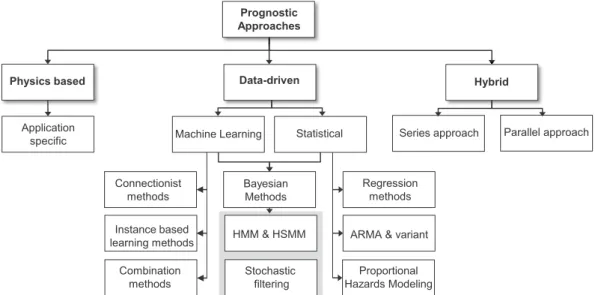
According to above discussions, prognostics approaches can be broadly categorized as
physics based, data-driven, and hybrid approaches (see Fig. 1.8).
Physics based
Application specific
Hybrid
Series approach Parallel approach Data-driven
Machine Learning Statistical
Connectionist methods Regression methods Combination methods Instance based
learning methods ARMA & variant
Proportional Hazards Modeling HMM & HSMM Stochastic filtering Prognostic Approaches Bayesian Methods
Figure 1.8: Classification of prognostics approaches
Among these categories, physics based approaches require modeling POF progression, and can produce precise results. As compared to data-driven methods, they need less
data, however, they are component / defect specific [63]. Building an analytical model
can be hard or even impossible for higher system level.
On the other hand, data-driven approaches are considered as model free, because they do not require any mathematical formulation of the process. They solely depend on sufficient run-to-failure data. The main strength of data-driven approaches is their ability to transform high dimensional noisy data into lower dimensional information for
diagnostic / prognostics decision [60]. They can be a good choice when it is hard to
build POF model of complex non-linear system. But, gathering enough CM data is not always possible, and the applicability of data-driven approaches is limited. They are also known as black-box approaches, and are not suitable for applications that require
transparency (e.g. credit card, earthquake, etc.) [131].
A hybrid of physics based and data-driven approaches could be a suitable choice to benefit from both categories. This area is also growing rapidly and several works have been published in recent years. Although with hybrid approach, reliability and accuracy
of prognostics model is gained significantly [226], but in parallel such methods can have
higher computational cost which makes them difficult for some applications.
prognostics approach either physics based, data-driven or hybrid, they are subject to
particular assumptions [178]. In addition, each approach has its own advantages and
disadvantages, which limits their applicability. Thereby, for a particular application (either for system level or for component level) a prognostics approach should be selected by considering two important factors: 1) performance and 2) applicability.
1.2.4.2 Usefulness evaluation - criteria
In general, prognostics domain lacks in standardized concepts, and is still evolving to attain certain level of maturity for real industrial applications. To approve a prognostics
model for a critical machinery, it is required to evaluate its performancesa priori, against
certain issues that are inherent to uncertainty from various sources. However, there are
no universally accepted methods to quantify the benefit of a prognostics method [191],
where, the desired set of prognostics metrics is not explicit and less understood. Methods to evaluate the performances of prognostics have acquired significant attention in recent
years. From a survey, [171, 173] provided a functional classification of performance
metrics, and categorize them into four classes.
1. Algorithm performance: metrics in this category evaluate prognostics model per-formance by errors obtained from actual and estimated RUL. Selection among competitive models is performed by considering different accuracy and precision criteria, e.g. Mean Absolute Percentage Error (MAPE), standard deviations, etc. 2. Computational performance: metrics in this category highlight the importance of computational performance of prognostics models, especially in case of criti-cal systems that require less computational time for decision making. Therefore, for a particular prognostics approach computational performance can be easily measured by CPU time or elapsed time (or wall-clock time).
3. Cost Benefit Risk: metrics in this category are related to cost benefits that are influenced by accuracy of RUL estimates. Obviously, operational costs can be reduced if RUL estimates are accurate. Because, this will result in replacement of fewer components before the need and also potentially fewer costly failures
[171]. For example, metrics in this class can be the ratio of mean time between
failure (MTBF) and mean time between unit replacement (MTBUR), return on investment (ROI), etc.
4. Ease of algorithm Certification: metrics in this category are related to the
assur-ance of an algorithm for a particular application (see [171] for details).
From the above classification, Cost Benefit Risk metrics have a broad scope, and obvi-ously it is hard to quantify probable risks that are to be avoided. The Ease of algorithm Certification metrics are related to algorithm performance class, because if the prognos-tics model error / confidence is not mastered, it can not be certified.
In addition to above classification, a list of off-line metrics is also proposed by [171,173]
1.2 Prognostics approaches 21 this includes metrics of: accuracy and precision, prognostics horizon, prediction spread, horizon / prediction ratio, which are again related to algorithm performance class. Therefore, finally this thesis focuses only on metrics from algorithm and computational performance classes for prognostics model evaluation (i.e., class 1 and 2).
As far as applicability of the prognostics approach is concerned, thanks to the
discus-sions on the application point of view for each prognostics approach (in sections 1.2.1.2,
1.2.2.3,1.2.3.3) one can point out important criteria for applicability assessment:
• requirement of degradation process model;
• failure thresholds;
• generality or scope of the approach;
• learning experience, i.e., run-to-failure data;
• transparency or openness.
• modeling complexity and computation time.
1.2.4.3 Prognostics approach selection
According to above discussions, in order to select a prognostics approach, performance and applicability factors are assessed upon different criteria (based on previous survey).
An intervalI = [1,5] is considered to assign weights for each approach according to the
given criteria, where 1 representsminweight and 5 representsmaxweight. For example
in Table 1.2, consider the first entry “without degradation process model”
(applicabil-ity factor). For this criteria, data-driven approach has max weight (i.e., 5), because it
does not require any explicit model of degradation process for prognostics. Similarly,
physics based approach has been assigned min weight (i.e., 1), as it is dependent on
mathematical model of degradation process. In this manner, weights for each criteria
are carefully given for both factors (i.e., applicability and performance) in Table 1.2,
and are further averaged to finally select a particular prognostics approach. For more clarity, a plot of averaged weights in terms of applicability vs. performance is also
shown in Fig. 1.9. The assessment clearly shows that data-driven methods have higher
applicability as compared to other approaches, but performances need further improve-ment. Consid