Stochastic analysis of packet-pair probing for
network bandwidth estimation
Kyung-Joon Park
a, Hyuk Lim
b,*, Chong-Ho Choi
aa
School of Electrical Engineering and Computer Science, Seoul National University, Shinlim, Kwanak, Seoul 151742, Republic of Korea
b
Department of Computer Science, University of Illinois, Urbana-Champaign, IL, United States
Available online 28 November 2005
Abstract
In this paper, we perform a stochastic analysis of the packet-pair technique, which is a widely used method for estimat-ing the network bandwidth in an end-to-end manner. There has been no explicit delay model of the packet-pair technique primarily because the stochastic behavior of a packet pair has not been fully understood. Our analysis is based on anovel insight that the transient analysis of the G/D/1 system can accurately describe the behavior of a packet pair, providing an explicitstochastic model. We first investigate a single-hop case and derive an analytical relationship between the input and the output probing gaps of a packet pair. Using this single-hop model, we provide a multi-hop model under an assumption of a single tight link. Our model shows the following two important features of the packet-pair technique: (i) The difference between the proposed model and the previous fluid model becomes significant when the input probing gap is around the characteristic value. (ii) The available bandwidth of any link after the tight link isnot observable. We verify our model via ns-2 simulations and empirical results. We give a discussion on recent packet-pair models in relation to the proposed model and show that most of them can be regarded as special cases of the proposed model.
Ó2005 Elsevier B.V. All rights reserved.
Keywords: Packet-pair technique; Bandwidth estimation; M/D/1 queue; Transient analysis
1. Introduction
To improve the performance of the Internet applications in various aspects, it is crucial to under-stand and exploit useful properties of an end-to-end path. For example, the available bandwidth is one such characteristic, which can be used in numerous
ways [1,2]: in many bandwidth-sensitive
applica-tions such as peer-to-peer applicaapplica-tions and on-demand multimedia streaming applications, a client will benefit if it is connected to a peer via a path with sufficient available bandwidth. Further, the perfor-mance of overlay networks can be improved if we can estimate the available bandwidth between nodes.
Now, we formally introduce two important char-acteristics of an end-to-end path: the bottleneck
capacity and the available bandwidth. Consider a
pathP as a set of links that forward packets from a sender S to a receiverR. Assume that the path
P is fixed and unique for the duration of the
1389-1286/$ - see front matter Ó2005 Elsevier B.V. All rights reserved. doi:10.1016/j.comnet.2005.09.037
* Corresponding author. Tel.: +1 217 244 1481.
E-mail addresses: [email protected](K.-J. Park),
[email protected] (H. Lim), [email protected] (C.-H. Choi).
measurement. LetMdenote the number of links in
P, then each link i, i= 1,. . .,M transmits packets with a constant rate of CiMb/s, which is referred to as thelink capacity. Then, thebottleneck capacity of pathPis
CP¼ min
i¼1;...;MCi
and the link withCP is called thenarrow link. Also,
if we letuidenote the utilization of linkiover a cer-tain interval, the available bandwidth of pathPis
AP¼ min
i¼1;...;M½Cið1uiÞ
and the link with AP is called the tight link. Note
that the tight link may be different from the narrow link in general. A more detailed explanation of the bottleneck capacity and the available bandwidth can be found in[2].
There has been a lot of research on the problem of measuring the bottleneck capacity and the avail-able bandwidth in an end-to-end manner. However, designing an accurate mechanism to measure the network bandwidth in an end-to-end path is chal-lenging since the Internet is a very complex dynamic system. A general way of active bandwidth measure-ment is to injectprobingpackets into an end-to-end path and observe their behavior to estimate the bot-tleneck capacity and the available bandwidth. One of the most popular mechanisms is the packet-pair technique [3–5], in which a source sends multiple packet pairs to a receiver. Each packet pair usually consists of two probing packets of the same size. The inter-packet dispersion between these two prob-ing packets changes accordprob-ing to path characteris-tics such as link capacities and cross-traffic. (Note that cross-traffic represents all the traffic in the path except the probing packets.) Hence, the relationship between the inter-packet dispersion at the sender and that at the receiver is exploited to estimate the end-to-end network bandwidth. Hereafter, we use the input/output probing gap and the inter-packet dispersion at the sender/receiver interchangeably.
The packet-pair technique has been extensively studied for network bandwidth estimation. Actu-ally, many tools for measuring the bottleneck capac-ity and the available bandwidth are based on the packet-pair technique[1,2,6–13]. However, most of these measurement methods rely on qualitative aspects or empirical results instead of an analytical model. Hence, the establishment of an accurate model of the packet-pair technique is of fundamen-tal importance for designing efficient bandwidth
estimation tools. Recently, a deterministic packet-pair model has been developed in[8]. Yet, this deter-ministic model assumes fluid cross-traffic with a constant rate and consequently ignores the stochas-tic nature of cross-traffic. More recently, Liu et al.
[14] has given a stochastic analysis of packet pair/ train probing, which provides upper and lower bounds of the relationship between the input and output probing gaps using a sample-path analysis under mildassumptions.
The main contribution of this paper is a deriva-tion of a stochastic model of the packet-pair tech-nique, which accurately captures the stochastic nature of cross-traffic. Unlike [14], we derive an
explicit model that shows a mathematical
relation-ship between the input and the output probing gaps. There has been no explicit delay model of the packet-pair technique, mainly because the stochastic behavior of a packet pair has not been fully under-stood. Our analysis is based on anovelinsight that the relationship between the input and the output probing gaps of a packet pair is governed by the transient behavior of a queueing system. Hence, under a reasonable assumption of Poisson cross-traffic, we give a stochastic delay model of the packet-pair technique via the transient analysis of the M/D/1 system.
First, we investigate a single-hop case and derive a stochastic delay model, which describes the ana-lytical relationship between the input and the output probing gaps of a packet pair. Then, we examine a multi-hop case and derive an explicit multi-hop model under an assumption of a single tight link. We validate the proposed model via ns-2 simula-tions and empirical results. Our model shows the following two important features of the packet-pair technique: (i) The difference between the proposed model and the previous fluid model becomes signif-icant when the input probing gap is around the characteristic value. (ii) The available bandwidth of any link after the tight link is not observable. Based on our analysis, we discuss recent packet-pair models in relation to the proposed model and show that most of them can be regarded as special cases of the proposed model.
The rest of the paper is organized as follows: In Section2, we provide preliminaries for the problem addressed in the paper. In Sections 3 and 4, we introduce a stochastic model, which can capture the essential stochastic nature of cross-traffic. In Section5, we validate the stochastic model through
the analysis, we present important features of the packet-pair technique and discuss several recent packet-pair models in relations to the proposed model in Section6. Finally, the conclusion follows in Section7.
2. Preliminaries
In this section, we explain how the packet-pair technique works in detail. Then, we introduce the deterministic packet-pair model in[8]. A single-hop deterministic model of the packet-pair technique was proposed in [8] under the assumption of fluid cross-traffic with a constant rate and consequently, the stochastic nature of cross-traffic was ignored.
The packet-pair technique works as follows: A source sendspacket pairsto a receiver. Each packet pair consists of two probing packets, usually of the same size. The time dispersion between these two packets changes according to path characteristics such aslink capacities andcross-traffic as they tra-verse the path. Hence, the relationship between the inter-packet dispersion at the sender and that at the receiver is exploited to obtain information on network bandwidth. The inter-packet dispersion Din at the sender is defined as the interval between the departure of the first probing packet from the sender and that of the second probing packet. In a similar manner, the inter-packet dispersion Dout at the receiver is defined as the interval between the arrival of the first probing packet at the receiver and that of the second probing packet. Our main concern here is how to establish an analytical rela-tionship betweenDoutandDin.
Consider a single link with capacityC. The sen-der at one end of the link transmits a packet pair to the receiver at the other end. The size of each probing packet is Lp bytes. Let t0denote the time when the first probing packet arrives at the queue. Also, letqdenote the amount of cross-traffic already in the queue whent=t0.Fig. 1illustrates the arrival and departure of a packet pair on a single link. In the figure,Tdenotes the interval between the arrival of the first probing packet and the departure of the second probing packet, and X(t0,Din) denotes the amount of cross-traffic arrived during [t0,t0+Din].
Under the assumption of fluid cross-traffic, the second probing packet will see the server busy or idle according to whether the server has been fully utilized or not during [t0,t0+Din]. The case of a busy server is given inFig. 1(a). Similarly, the case of an idle server is presented inFig. 1(b). Note that X(Din) is used instead ofX(t0,Din) in the figure since X(t0,Din) is independent of t0 under the fluid assumption. Also, we should note that, without the assumption of fluid cross-traffic with a constant rate, it will be the last busy period in [t0,t0+Din] that determines whether the server is busy or idle when the second probing packet arrives. The server will be busy if the second probing packet arrives before the end of the last busy period. On the other hand, if the last busy period ends before the second probing packet arrives, the server will be idle.
Under the assumption of fluid cross-traffic with a constant rater,X(t0,Din) yields a deterministic value ofrDinand the following relationship between Dout and Din can be derived depending on whether the link is fully utilized or not[8]:
Dout¼ r CDinþ Lp C; Din6D ¼Lpþq Cr ; Dinq C; otherwise. ( ð1Þ
From(1), we know that the graph of (Din,Dout) con-sists of two line segments and the change of slope occurs at Din¼D ¼Lpþq
Cr
, which is termed as
thecharacteristic value. Further, if we letDcdenote
the value ofDinsuch thatDin=Dout, thenDc¼ Lp
Cr, which is termed as the critical value. Note that we can obtain the available bandwidthAonce we know Dc by A=Cr=Lp/Dc. Since q0 under the assumption of fluid cross-traffic, DcD* and we further have A=CrLp/D*. Actually, many measurement algorithms seek the available band-width A by estimating the characteristic value D*
[1,8,10,13]. However, we can easily suspect that
con-siderable modeling error is introduced in(1)by the assumption of fluid cross-traffic with a constant rate. In this paper, we consider X(t0,Din) as a sto-chastic process and derive a model that depicts the relationship betweenDout andDin more accurately. Then, we discuss recent packet-pair models in relation to the proposed model.
3. Packet-pair delay model: single-hop case
In this section, our primary concern is to derive a single-hop relationship between the input and the output probing gaps under an assumption of sta-tionary Poisson cross-traffic. Based on this assump-tion, we show that the transient analysis of the M/ D/1 system can accurately describe the behavior of a packet pair. By adopting the M/D/1 analysis, we only consider packets of the same size in cross-traf-fic. Since the packet size distribution of the Internet traffic is known to be multi-modal [15], M[X]/D/1 analysis which allows batch arrivals would be more complete [16]. However, the M/D/1 analysis plays an essential role in the M[X]/D/1 analysis. Also, the M/D/1 analysis by itself gives a valuable insight, namely that the queueing theory can be successfully applied to the modeling of the packet-pair technique for bandwidth measurement. For these reasons, the focus here is on the M/D/1 analysis of the packet-pair technique.
Here, we adopt the transient analysis of the M/ D/c queueing system in[17]. First, we give our ratio-nale as to how the behavior of a packet pair can be described by the transient queueing analysis. Then, based on the M/D/1 analysis, we develop the state vector in a transient regime and the concept of the
virtual waiting time in order to depict the wait-ing time of the second probwait-ing packet. Finally, we give a stochastic delay model of the packet-pair technique.
3.1. The key idea of M/D/1 modeling
Here, we assume that the cross-traffic is a station-ary Poisson process in the time scale of interest. The stationary assumption for the Internet traffic is typ-ical in the literature and is known to be empirtyp-ically acceptable over intervals of several minutes up to a few hours[18,19].
When the first probing packet arrives at the queue at t=t0, assume that there are q1 packets already in the queue and one in service with the residual service time d. (If there is no packet in ser-vice at t=t0, d= 0.) In a similar manner, assume that there areq2packets already in the queue when the second probing packet arrives at the queue. Let W1and W2denote the waiting times (in queue) of the first and the second probing packets, respec-tively. Since both the service times of the first and the second probing packets equal to Lp/C, we have
DoutDin¼ ðW2þLp=CÞ ðW1þLp=CÞ
¼W2W1. ð2Þ
The key insight is that, from the viewpoint of the second probing packet, W2is the transient waiting time in queue of the M/D/1 system with initially q1+Lp/Lc+ 1 packets, where Lcis the packet size of cross-traffic.1 The rationale is as follows: Just after the arrival of the first probing packet, i.e.,
t¼tþ0, there are a total of q1+Lp/Lc+ 1 =:N0 packets in the system including one possibly in ser-vice. Now, the overall system can be considered as the M/D/1 queue with initially N0 packets in the system, which begins to evolve at t=t0. Hence, without loss of generality, lett0= 0. Then, the wait-ing time W2 of the second probing packet exactly corresponds to that of a packet which arrives at the M/D/1 system at t=Din. Consequently, the problem now becomes how to find the transient waiting time of the M/D/1 system att=Dininitially holdingN0packets.
1
In order to make the problem more tractable, it is assumed thatLp/Lcis an integer and the round-off effect is ignored.
3.2. Waiting time distribution of the second probing packet
First, we introduce the state vector of the M/D/1 system. Let pj(t) denote the probability of the system holding j packets at time t. Then, the state vectorp(t) =: (p0(t),p1(t),p2(t),. . .) can be obtained as follows:
Lemma 1. (i)When t2(0, D] where D = Lc/C,
pjðtÞ ¼ ðktÞjN0þKðtÞ ðjN0þKðtÞÞ!e kt; jPN 0KðtÞ; 0; j<N0KðtÞ; (
where N0= q1+ Lp/Lc+ 1, k is the packet arrival rate of cross-traffic, and K(t) is the number of packets that have left the system by t.
(ii)When t>D, pðtÞ ¼pðtmodDÞPbt=Dc; where P¼ ekD kDekD . . . ðkDÞj1 ðj1Þ!e kD . . . ekD kDekD . . . ðkDÞj1 ðj1Þ!e kD . . . 0 ekD . . . ðkDÞj2 ðj2Þ!e kD . . . 0 0 ekD . . . . . . .. . .. . .. . .. . . . . 0 B B B B B B B B B @ 1 C C C C C C C C C A
Proof. SeeAppendix. h
Hence, we can obtain the state vector when the sec-ond probing packet arrives at the queue, i.e.,p(Din) for any arbitrary value of DinfromLemma 1.
Now, we derive the waiting time distribution of the second probing packet. Let the random variable W(T) denote the waiting time of an arbitrary packet which arrives at an M/D/1 queue att=T> 0. We will call this packet a virtual packet. Then, we have W2=W(Din) with initially holdingN0packets in the system. Hence, if we can find the distribution of W(Din) for any given value of Din, then it will be straightforward to obtain the relationship between DoutandDinfrom (2). The virtual waiting time dis-tribution P(W(Din)6kDv) for all k2N and
v2(0,D], can be determined by concentrating on
the queueing position of the virtual packet at
t=Din+Dv. If we define the random variable
NDinðtÞ as the number of packets arriving before Dinthat are still in the system att, then the cumula-tive distribution function (CDF) of the waiting time W(Din) is as follows: Proposition 1. The CDF FDinðxÞ ¼PfWðDinÞ6xg is FDinðxÞ ¼ P bx DcN0þKðyþDÞ j¼0 ðkDinÞj j! e kDin; y60; Pbx Dc j¼0 Qbx DcjðyÞ ðkzÞj j! e kz; otherwise; 8 > > > > < > > > > :
where y :=DinD + (xmodD), z := D(xmodD), andQmðtÞ:¼Pim¼þ01piðtÞ.
Proof. See Appendix. h
3.3. M/D/1 delay model of packet-pair probing By combining all these results, we derive a delay model of packet-pair probing in a single hop. First, for given value ofDinandq1,
E½W2jq1 ¼E½WðDinÞjq1 ¼
Z 1
0
ð1FDinðxÞÞdx.
Here, FDinðxÞ can be obtained from Proposition 1
withN0=q1+Lp/Lc+ 1. Finally from(2),
E½Dout ¼DinþE½E½W2jq1 E½W1ðq1Þ. ð3Þ Note that we can calculate E½E½W2jq1 and E½W1ðq1Þin(3) by using the distribution of q1, the steady-state solution of the M/D/1 queue. An effi-cient algorithm to obtain the steady-state solution can be found in, for example[20].
Now, in order to enhance our understanding of the proposed model (3), consider the two extreme cases where Din!0 and Din! 1. First, we have the following result whenDin!0:
Proposition 2. When Din1/k, the relationship between the input and the output probing gaps becomes
E½Dout ¼ r CDinþ
Lp
C þoðDinÞ.
Proof. From the basic property of the Poisson
process, whenDin1/k,
Að0;DinÞ ¼ 1; with probabilitykDinþoðDinÞ;
0; with probability 1kDinþoðDinÞ.
Then, for givenq1,
FDinðxÞ ¼ ð1kDinÞIðxN0DÞ þkDinIðx ðN0þ1ÞDÞ þoðDinÞð1IðxMDÞÞ;
whereI(Æ) is the indicator function andMis a suf-ficiently large number independent ofDin. Hence,
E½W2jq1 ¼ Z 1 0 ð1FDinðxÞÞdx ¼kDDinþN0DþoðDinÞ. By usingW1= (N0Lp/Lc)D, E½Doutjq1 Din¼E½W2jq1 W1 ¼kDDinþLpD=LcþoðDinÞ. ð4Þ Since Dout is independent of q1, with D=Lc/C and r=kLc, (4) becomes E½Dout ¼CrDinþ
Lp
Cþ oðDinÞ. h
Here, we should note that the result inProposition 2
is identical to the full-utilization case of the deter-ministic model in(1).
WhenDin! 1, we have the following result:
Proposition 3. When Din! 1, E½Dout Din; where f(t)g(t) represents f(t)/g(t)!1 as t! 1. Proof. From(2), E½Dout Din¼E½W2 E½W1 ¼E½E½W2ðq2Þjq1 E½W1ðq1Þ.
As Din! 1, W2 becomes independent of N0 and consequently, E½W2 E½W1. Hence, when Din is very large,E½Dout Din. h
Here, again note that the result inProposition 3
is identical to the under-utilization case of the deter-ministic model in (1). Hence, from Propositions 2
and 3, the deterministic model(1)can be considered
as anasymptoteof the proposed stochastic model. The relationship in Proposition 3 can also be explained in a qualitative manner from a physical viewpoint. The difference betweenE½W2andE½W1 results from the first probing packet itself. The arri-val of the first probing packet perturbs the M/D/1 system as it acts as an additional packet in the initial state of the system. Consequently, this perturbation makesE½W2PE½W1. The effect of the first probing packet will eventually disappear as Din! 1, and we haveProposition 3.
4. Stochastic packet-pair model: multi-hop case
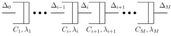
Here, we derive a model for a multi-hop path which has a single tight link. Consider M links in
an end-to-end path as in Fig. 2. Let Ci, Xi, q1,i, and q2,i denote, respectively, the link capacity, the amount of cross-traffic, and the queue length of the first and the second probing packets on the ith link, 16i6M. Also, the average packet sending
rate of Xi and the link utilization of link i are denoted bykiandui, respectively. Furthermore, let Di denote the inter-departure time from the ith queue. Then Di becomes the inter-arrival time at the (i+ 1)th queue, and Din=D0 and Dout=DM. With the above notations, the available bandwidth of the ith link is Ai=Ci(1ui) and the available bandwidth of a path is As where s= argiminAi. The assumption of a single tight link represents the case whereAsAifori= 1,. . .,M,i5s.
Similarly as the single-hop case in(2), we have DiDi1¼W2;iW1;i; i¼1;. . .;M. ð5Þ Hence, by adding all the terms on each side from i= 1 toM, we have DoutDin¼DMD0¼ XM i¼1 ðW2;iW1;iÞ. Then, E½Dout ¼DinþX M i¼1 E½W2;iW1;i ¼DinþX M i¼1 E½E½W2;iW1;ijq1;i. ð6Þ
Now, we first consider a two-hop case and extend the result to the general multi-hop path.
4.1. Two-hop case
Before dealing with a general multi-hop path, we first consider a two-hop path, i.e.,M= 2 inFig. 2. First, we assume that D1<D2. This implies that the available bandwidth of the path is that of the second link. From(6)with M= 2, we have E½Dout ¼DinþE½W2;1W1;1 þE½W2;2W1;2. Now, we derive an explicit relationship between E½Dout and Din under the assumption of a single tight link. If we further assume that D1D2 and
Din is around D2, then DinD1. Hence, we have E½W2;1W1;1 0 fromProposition 3. In this case, we have
E½Dout DinþE½W2;2W1;2. ð7Þ WhenD0is aroundD1,DinD2 and
E½D1 DinþE½W2;1W1;1. Also, E½Dout u2E½D1 þ Lp C2 . Hence, E½Dout u2ðDinþE½W2;1W1;1Þ þ Lp C2 . ð8Þ
Both (7) and (8)can be solved in the same manner
as the single-link case. Note that, in finding the available bandwidth along the path, only (7) is needed. Also, note that (7) and (8)are valid under the assumption of D1D2. As D1 approachesD2, i.e., the available bandwidth of the first link ap-proaches that of the second link, the assumption is no longer valid, and(7) and (8)become inaccurate. Now, let us consider the case ofD1>D2, i.e., the available bandwidth of the path is that of the first link. Similarly to the case of D1<D2, we further assume D1D2. When Dinis around D1, similarly as in (7)we have
E½Dout DinþE½W2;1W1;1. ð9Þ WhenDinis aroundD2,
E½D1 DinþE½W2;1W1;1.
we also haveE½Dout E½D1withD1D2. Hence, E½Dout DinþE½W2;1W1;1. ð10Þ
From (9) and (10), we know that the characteristic
value of the second link, i.e., D2 is not observable via the packet-pair technique when the available bandwidth of the first link is smaller than that of the second link. We will also verify this phenome-non in the simulations in Section 5.
4.2. Multi-hop case
By extending the two-hop analysis to theM-hop case, E½Dout ¼DinþX M i¼1 E½W2;iW1;i DinþX s i¼1 E½W2;iW1;i;
where thesth link has the minimum available band-width. Hence, based on the packet-pair technique, we cannot observe the characteristic value of any link after the tight link. In other words, any link after the tight link does not affect the relationship between the input and the output probing gaps. Consequently, the available bandwidth of any link after the tight link is not observable in an end-to-end manner if we use the packet-pair technique. We can obtain the information only on the available bandwidth of theith link wherei6s.
If we are concerned only with obtaining the avail-able bandwidth of an end-to-end path, it is sufficient to observe the behavior of the packet-pair technique in the vicinity of Din¼Ds. If we assume that Ds Di, i= 1,. . .,M, i5s, i.e., there is a single tight link as in the cases of(7) and (9), we can derive the following approximate model for the multi-hop path: E½Dout ¼DinþX M i¼1 E½W2;iW1;i DinþE½W2;sW1;s. ð11Þ The multi-hop model(11)shows that we can obtain the available bandwidth of the path from the local analysis which is identical to the single-hop case in
(3)when we assume a single tight link.
4.3. Discussion on the proposed model
Here, we discuss the impact of the proposed packet-pair model on available bandwidth estima-tion. Since the multi-hop analysis is identical to the single-hop case when we are concerned only about the available bandwidth of the path under the assumption of a single tight link, we discuss the single-hop model(3)in relation to the available bandwidth estimation. We show the difference between the proposed model(3)and the determinis-tic model(1)inFig. 3. The figure shows that avail-able bandwidth estimation algorithms based on(1)
may give an inaccurate estimate of the characteristic valueD*because of the modeling error. Further, the error is most significant when Din=D* (24 ms in
Fig. 3). This error between the deterministic and
the stochastic models has been also identified and termed as the probing bias in [14]. The influence of the probing bias on available bandwidth mea-surement is significant since the probing bias makes it difficult to estimate the characteristic value by observing the relationship betweenDoutandDin.
5. Model validation
In this section, we validate our stochastic model vians-2 simulations and experimental results.
5.1.ns-2 simulations for single-hop topology
We perform simulations for a single-hop topol-ogy composed of two drop-tail routers that are con-nected via a link with the capacity of 1 Mb/s and a propagation delay of 15 ms. First, we investigate the deterministic model(1). In the simulation, the cross traffic consists ofNPareto sources, and each source generates packets at the rate of 32 Kb/s with the packet size ofLc= 50 bytes.Fig. 4(a) and (b) show DinDoutversusDinforN= 7 and 15, respectively, where Dout:¼E½Dout. The sizes of probing packets are 500, 1000, and 1500 bytes, respectively. Note that we introduce DinDout¼:Kout to highlight the change of oDout
oDin around the characteristic value
D ¼Lpþq
Cr
. Each data point is an average value of 300 trials. The solid lines are obtained from the deterministic model in (1) with q= 0. We can see that the simulation data asymptotically converges to the analytical values. However, the modeling error aroundDin=D*becomes larger as the link uti-lization or the probing packet size increases. oKout
oDin
changes smoothly aroundDin=D*in the simulation results while it changes abruptly at Din=D*in the deterministic model. This implies that the stochastic nature of cross-traffic makes it difficult to find the value ofD*in practice.
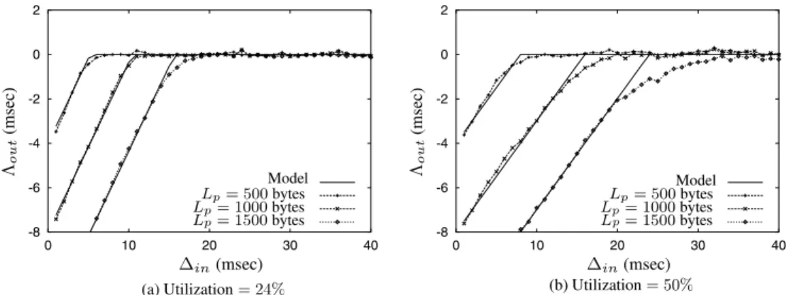
Now, we validate the stochastic model in (3).
Figs. 5–7showKoutversusDinfor Poisson,
exponen-tial ON–OFF, and Pareto ON–OFF cross-traffic, respectively. Even though we have assumed Poisson cross-traffic in our analysis, we perform simulations with exponential ON–OFF and Pareto ON–OFF cross-traffic to see the effect of the cross-traffic dis-tribution. Each figure shows the result for different sizes of probing packets (Lp= 500, 1000, and 1500 bytes) with the utilization of 24% and 50%, respec-tively. In all the simulations, we use Lc= 50 bytes for the packet size of cross-traffic. In Fig. 5, we can see that each of the simulation results agrees very well with the stochastic model in (3). This is because the Poisson cross-traffic is used both in the model and the simulations. Now, we consider the exponential ON–OFF sources in Fig. 6. In
Fig. 6, the Poisson cross-traffic is used for the model
as in Fig. 5 while the exponential ON–OFF cross traffic is employed in the simulation. Accordingly, we can see that there exist some errors between the model and the simulation data. Note that the slope ofKoutchanges more slowly aroundDin=D* in the simulation data than in the model. Next, we consider the case of the Pareto ON–OFF
cross-traf-0 0.2 0.4 0.6 0.8 1 0 10 20 30 40 50 60 Δin (ms) Difference (ms)
Fig. 3. Difference between the proposed and the deterministic models.
fic inFig. 7. Similarly as inFigs. 6 and 7show some error around Din=D* for the same reason. Note that the variance of the Pareto ON–OFF traffic is even larger than that of the exponential ON–OFF traffic, andKoutchanges more slowly in the simula-tion data ofFig. 7than that ofFig. 6.
Now, we vary the packet size of the Poisson cross-traffic to investigate the effect of the packet size on the model accuracy.Fig. 8(a) and (b) show the simulation results ofKoutvs.Dinunder different link utilizations for the packet sizes of 50 and 500 bytes, respectively. When the packet size is 50 bytes,
Fig. 5.KoutversusDinfor the Poisson cross traffic in a single-hop topology.
Fig. 6. KoutversusDinfor the exponential ON–OFF cross-traffic in a single-hop topology.
we can verify from Fig. 8(a) that the proposed model is quite accurate. When the packet size is 500 bytes in Fig. 8(b), the proposed model still agrees quite well with the simulation result. Note that each point in Fig. 8 is an average value of 30,000 trials. We will also investigate the effect of the packet size in cross traffic with the empirical results in Section5.3.
5.2.ns-2 simulations for two-hop topology
We now validate the stochastic model for the two-hop topology, which is composed of three drop-tail routers that are connected via two links with capacity of either C1= 2 Mb/s and C2= 1 Mb/s (which corresponds to the case D1<D2) or C1= 1 Mb/s and C2= 2 Mb/s (which corre-sponds to the case D1>D2). The cross-traffic on the first link (the second link) is composed of 23 (15) Pareto sources that give an aggregate rate of r= 736 Kb/s (r= 480 Kb/s). The packet size Lc
of cross-traffic is 100 bytes. Fig. 9(a) and (b) show the analytical and simulation results for the cases of D1<D2 and D1>D2, respectively. In the case of D1<D2 (Lp= 1500 bytes, C1= 2 Mb/s, C2= 1 Mb/s), we can see two changes in ooKDout in
around Din¼D1¼9:5 ms and Din¼D2¼23:1 ms
in Fig. 9. Note that D2 gives the information on
the available bandwidth along the path. In the case of D1>D2 (Lp= 1500 bytes, C1= 1 Mb/s, C2= 2 Mb/s), we only see one change in ooKDoutin around Din¼D1¼23:1 ms. Hence, Fig. 9 shows that the multi-hop model in (11) agrees quite well around the largest characteristic value, which gives information on the available bandwidth of the path.
5.3. Empirical results in two-hop network
Here, we investigate the proposed stochastic model in a real network environment. The network is composed of three routersR1,R2, andR3that are
Fig. 8. Packet size effect of cross-traffic (Lp= 1500 bytes).
connected via two 100 Mb/s links and five hosts, denoted by l1, l2, and Hi, i= 1,. . ., 5, respectively, as depicted inFig. 10. Here, each host is a PC with a single 2.66 GHz processor and 1 GByte RAM that runs Redhat Linux Release 9.0 with the kernel version 2.4.20–31.9. The routers used in the experiments are Cisco 1700 Series. The path for which we injected the probing packets was
P:H1!R1!R2!R3!H3, which constitutes a two-hop path. Each of the experimental data points
in Figs. 11 and 12is an average of 5 trials.
The Poisson cross-traffic is generated and tra-verses the path from H5 to H4. Hence, the link l2:R2!R3becomes the tight link of the path P.
Fig. 11(a) and (b) show Kout for Lp= 500, 1000,
and 1500 bytes, when Lc is 250 bytes and the link utilization is 25% and 50%, respectively. We can see that the stochastic model agrees quite well with the experimental data in the figure. The pathPused in the experiments was composed of two links l1:R1!R2and l2:R2!R3, and the correspond-ing characteristic values of the link l1 are
Fig. 10. Topology used in the experiments.
Fig. 11.KoutversusDinwith the Poisson cross traffic ofLc= 250 bytes in the two-hop experiment.
D1¼Lp=C1¼40, 80, and 120ls forLp= 500, 1000, and 1500 bytes, respectively. Similarly, the charac-teristic values of link l2 when u= 25% (u= 50%) are D2¼Lp=ðC2r2Þ ¼160=3, 320/3, and 160ls (80, 160, and 240ls) for Lp= 500, 1000, and 1500 bytes, respectively. Since D1<D2, we can observe both D1 and D2 in Figs. 11 and 12 as in
Fig. 9(a). Note that the experimental data changes
smoothly around Din¼D2 as expected, and this makes it difficult to find D2. This difficulty is not apparent with the deterministic model in (1).
Fig. 12shows the results of the similar experiments
with Lc= 750 bytes. From the figure, we can see that the stochastic model follows the experimental data quite well. In summary, the experimental results show that the proposed model is quite accu-rate in a real environment even when the packet size of cross-traffic is large (Lc= 250 bytes inFig. 11and Lc= 750 bytes inFig. 12).
6. Related work
The packet-pair technique originally appeared in the seminal work by Jacobson [3], Keshav [4], and Bolot[5]. This early work was followed by extensive research into the packet-pair technique. Here, we investigate several recent models of the packet-pair technique for bandwidth measurement.
In[7], Dovrolis et al. proposed the following rela-tionship between the input and the output probing gaps: Di¼ siþd2i; Di16siþd1i; Di1þ ðd2i d 1 iÞ; otherwise; ( ð12Þ
wheresi andd1i denote the transmission delay and the queueing delay of the first probing packet at
theith link, respectively. Also,d2i denote any
addi-tional queueing delay of the second probing packet at theith link after the first probing packet has de-parted from the link. Hence, d2i ¼W2;i when Di1Psiþd1i, but d
2
i 6¼W2;i when Di16siþd1i. Under the fluid cross traffic with a constant rate, we have si=Lp/C, d1i ¼rDi1 when Di16 Lp Ciþd 1 i and d1i ¼d2i when Di1> Lp Ciþd 1 i. Hence, (12) ex-actly matches the deterministic model (1) under the assumption of fluid cross-traffic. Note that(12)
is more general than the deterministic model (1)
since (12) describes the stochastic relationship be-tween Di1 and Di. We can easily show that (12) can be transformed into(5)as follows: from the def-initions, we can easily know that d1i ¼W1;i and
siþd1i þd 2 i ¼Di1þW2;i when Di16siþd1i. When Di1Psiþd1i, we have d 1 i ¼W1;i and
d2i ¼W2;i. Hence, with these relationships, (12)can
be converted into(5).
As already explained, a deterministic packet-pair model was derived under an assumption of fluid cross-traffic in [8], which is a deterministic version of (12). As we have shown in Propositions 2 and 3, this deterministic model corresponds to an asymptote of the proposed M/D/1 model.
More recently, a stochastic analysis of packet pair/train has been given in [14], in which the fol-lowing upper and lower bounds for the single-hop case was derived based on a sample-path analysis
LðE½DoutÞ ¼ r CDinþ Lp C; Din6 Lp Cr; Din; otherwise; ( ð13Þ UðE½DoutÞ ¼ r CDinþ Lp C; Din6 Lp C; r CDinþDin; Lp C 6Din6 Lp r ; DinþLp C; otherwise. 8 > > < > > : ð14Þ
We can verify that(13)is identical to the determin-istic model (1), which is an asymptote of the sto-chastic model(3).
Furthermore, from (14), we have the following lower bound forKout¼DinE½Dout
LðKoutÞ ¼ ð1r CÞDin Lp C ; Din6 Lp C; r CDin; Lp C 6Din6 Lp r; Lp C; otherwise. 8 > > < > > : ð15Þ
Since E½E½W2jq1 in (3) is a decreasing function of Din, Kout is an increasing function of Din. Hence, we know from (15)that the upper bound in(14)is not very tight when Lp
C 6Din6 Lp
r. Overall, the sam-ple-path analysis in [14]has successfully shown the general characteristics of the packet pair/train prob-ing technique. Our analysis differs from the result of
[14]in that we have derived an explicit relationship under Poisson cross-traffic. Further, we have given a novel insight that the transient queueing analysis can accurately describe the behavior of a packet pair. This insight has a significant importance since it provides an effective way of modeling the packet-pair technique by using queueing theory.
7. Conclusion
In this paper, we have derived an explicit packet-pair model, which reflects the stochastic nature of cross-traffic. We have investigated the mathematical
relationship between the input and the output prob-ing gaps of a packet pair in the sprob-ingle-hop and the multi-hop cases under the assumption of stationary Poisson cross-traffic. We have shown that the pro-posed model agrees very well with thens-2 simula-tions and the empirical results. Based on the analysis, we have pointed out that most of the recent models of the packet-pair technique can be regarded as special cases of the proposed model. We expect that the proposed model will play an important role in developing a measurement mech-anism for estimating network bandwidth.
There remain several issues for future research work. In the analysis of developing a multi-hop model, we have made an assumption of a single tight link. However, this assumption will be unreal-istic if two or more links have nearly the same avail-able bandwidth. Hence, development of a multi-hop model without this assumption remains as future work. It is also necessary to carry out large-scale measurement on the Internet in order to verify the stochastic model with real network traffic. Exten-sion of the M/D/1 model to the M[X]/D/1 case is another future task to take account of the multi-modal distribution of the Internet traffic packet size.
Acknowledgements
This work has been supported in part by POSCO and the BK21 IT Program of the Korean Ministry of Education and Human Resources.
Appendix A
A.1. Proof of Lemma 1
Here, the proof is a slight modification of the result in [17]. Whent2(0,D] whereD=Lc/C, the only packets that may have left the system since t= 0 are those already in service at t= 0. There are initially N0=q1+Lp/Lc+ 1 packets at t= 0 and letK(t) denote the number of packets that have left the system by the time t. With the residual service timed,
KðtÞ ¼
1; ford6t6D
0; otherwise. (
Note thatd= 0 andK(t) = 1,t2(0,D] if there is no packet in service at t= 0. During the time interval
(0,t] there will be i new arrivals with probability
ðktÞi
i! e
kt. In order to havej customers in the system at timet, we needjN0+K(t) new arrivals during
(0,t], and consequently, for anyt2(0,D],
pjðtÞ ¼ ðktÞjN0þKðtÞ ðjN0þKðtÞÞ!e kt; jPN 0KðtÞ; 0; j<N0KðtÞ. 8 < :
When t>D, by conditioning on the number of
packets at timet,
pjðtþDÞ ¼PðNðtÞ ¼0ÞPðjarrivalsjNðtÞ ¼0Þ
þX
jþ1
i¼1
PðNðtÞ ¼iÞPðjþ1iarrivalsjNðtÞ ¼iÞ
¼p0ðtÞ ðkDÞj j! e kD þX jþ1 i¼1 piðtÞ ðkDÞjþ1i ðjþ1iÞ!e kD
for all j2N0. Let us define the transition matrix P= [pij] as follows: pij¼ ðkDÞj1 ðj1Þ!e kD; fori¼1; ðkDÞjiþ1 ðjiþ1Þ!e kD; for 26i6jþ1; 0; otherwise. 8 > > > < > > > : Then, pðtþDÞ ¼pðtÞP. ðA:1Þ
By applying (A.1) iteratively, we can determine
p(t+mD) for anym2Nas follows:
pðtþmDÞ ¼pðtÞPm
. ðA:2Þ
From(A.2), the following relation is obtained:
pðtÞ ¼pðtmodDÞPbt=Dc.
A.2. Proof of Proposition 1
Here, the proof adopts the result in[17]. LetN(t) denotes the number of packets in the system at time t. Since the arrival of the second probing packet is independent of any packet arrivals of cross traffic,
PðNðtÞ ¼ijsecond probing packet arrives at DinÞ ¼piðtÞ;
for 06t<Din. Since Din> 0 and 0 <v6D, epoch Din+Dvmust take place aftert= 0. Now we di-vide the problem into the following two cases: Dinv60 as Case 1 andDinv> 0 as Case 2. In
Case 1,Din+Dv2(0,D]. Therefore, att=Din+
packets that were already in the system at t= 0. Another group of packets arriving before the second probing packet are those which arrive in (0,Din). Let A(t1,t2) denote the number of packet arrivals in interval (t1,t2), then
NDinðDinþDvÞ ¼N0KðDinþDvÞ
þAð0;DinÞ;tv60. ðA:3Þ
In addition, we can obtain a relation between W(Din) and NDinðtÞ in the following way. Consider
the two cases:NDinðDinþDvÞ<k and NDinðDinþ DvÞPk. First, when NDinðDinþDvÞ<k,
(k1)D time units later we must have NDin ðDinþkDvÞ<k ðk1Þ ¼1. Consequently, we know that the virtual packet will not be in the queue
att=Din+kDv. Hence,
NDinðDinþDvÞ<k)WðDinÞ6kDv. ðA:4Þ
On the other hand, if NDinðDinþDvÞPk, the
virtual packet will remain in the queue at
t=Din+kDv. Consequently,
NDinðDinþDvÞPk)WðDinÞ>kDv. ðA:5Þ
By considering(A.4) and (A.5)together,
NDinðDinþDvÞ<k()WðDinÞ6kDv. ðA:6Þ
In terms of probabilities,(A.6)becomes
P½WðDinÞ6kDv ¼P½ND
inðDinþDvÞ<k. ðA:7Þ
From(A.3) and (A.7), whenDinv60,
PðWðDinÞ6kDvÞ ¼PðAð0;DinÞ
<kN0þKðDinþDvÞÞ.
Since A(0,Din) is Poisson, independent of N0 and
K(Din+Dv), PðWðDinÞ6kDvÞ ¼ X kN0þKðDinþDvÞ1 j¼0 ðkDinÞj j! e kDin; whenDinv60.
When Dinv> 0 in Case 2, we have
Din+Dv>D. Hence, we use the fact that all
packets that were in service att=Dinvwill have left the system att=Din+Dv, whereas all pack-ets that were waiting for service at t=Dinv will still be in the system at t=Din+Dv. Let Lq(t) denote the queue length at time t, then at t= Din+Dv there will be exactly Lq(Dinv) +
A(Dinv,Din) packets in the system that arrived before the second probing packet. Hence, when Dinv> 0, we have
NDinðDinþDvÞ ¼LqðDinvÞ þAðDinv;DinÞ.
By conditioning on the number of arrivals during [Dinv,Din], we get
PðWðDinÞ6kDvjAðDinv;DinÞ ¼jÞ ¼PðLqðDinvÞ<kjÞ;
when Dinv> 0. Since A(Dinv,Din) is indepen-dent of Lq(Dinv), PðWðDinÞ6kDvÞ ¼X k1 j¼0 PðLqðDinvÞ<kjÞ ðkvÞj j! e kv;
whenDinv> 0. By using the cumulative probabil-ity QmðtÞ ¼Pmi¼þ01piðtÞ, PðWðDinÞ6kDvÞ ¼X k1 j¼0 Qkj1ðDinvÞðkvÞ j j! e kv. ðA:8Þ
Note that Qkj1(Dinv) can be easily calculated
from Lemma 1. By substituting x=kDv and
k¼ bx
Dc þ1 in (A.8), the waiting time distribution
FDinðxÞ ¼PðWðDinÞ6xÞis obtained as follows:
FDinðxÞ ¼ P bx DcN0þKðyþDÞ j¼0 ðkDinÞj j! e kDin; y 60; Pbx Dc j¼0 Qbx DcjðyÞ ðkzÞj j! e kz; otherwise; 8 > > > > < > > > > :
where y:=DinD+ (xmodD) and z:=D
(xmodD).
References
[1] M. Jain, C. Dovrolis, End-to-end available bandwidth: measurement methodology, dynamics, and relation with TCP throughput, IEEE/ACM Transactions on Networking 11 (4) (2003) 537–549.
[2] R.S. Prasad, M. Murray, C. Dovrolis, K.C. Claffy, Band-width estimation: metrics, measurement techniques, and tools, IEEE Network 17 (6) (2003) 27–35.
[3] V. Jacobson, Congestion avoidance and control, in: Pro-ceedings of ACM SIGCOMM, 1988.
[4] S. Keshav, A control-theoretical approach to flow control, in: Proceedings of ACM SIGCOMM, 1991.
[5] J.C. Bolot, Characterizing end-to-end packet delay and loss in the Internet, in: Proceedings of ACM SIGCOMM, 1993, pp. 289–298.
[6] R.L. Carter, M.E. Crovella, Measuring bottleneck link speed in packet-switched networks, Performance Evaluation 27–28 (1996) 297–318.
[7] C. Dovrolis, P. Ramanathan, D. Moore, What do packet dispersion techniques measure? in: Proceedings of IEEE INFOCOM, 2001, pp. 905–914.
[8] N. Hu, P. Steenkiste, Evaluation and characterization of available bandwidth probing techniques, IEEE Journal of Selected Areas in Communications 21 (6) (2003) 879–894. [9] K. Lai, M. Baker, Measuring bandwidth, in: Proceedings of
IEEE INFOCOM, 1999, pp. 235–245.
[10] B. Melander, M. Bjorkman, P. Gunningberg, A new end-to-end probing and analysis method for estimating bandwidth bottlenecks, in: Proceedings of IEEE Global Internet Sym-posium, 2000.
[11] V. Paxson, End-to-end Internet packet dynamics, IEEE/ ACM Transactions on Networking 7 (3) (1999) 277– 292.
[12] V.J. Ribeiro, R.H. Riedi, R.G. Baraniuk, J. Navratil, L. Cottrell, Pathchirp: efficient available bandwidth estimation for network paths, in: Proceedings of Passive and Active Measurement Workshop (PAM), 2003.
[13] J. Strauss, D. Katabi, F. Kaashoek, A measurement study of available bandwidth estimation tools, in: Proceedings of ACM Internet Measurement Conference (IMC), 2003. [14] X. Liu, K. Ravindran, B. Liu, D. Loguinov, Single-hop
probing asymptotics in available bandwidth estimation: sample-path analysis, in: Proceedings of ACM Internet Measurement Conference (IMC), 2004.
[15] The Cooperative Association for Internet Data Analysis. URL:http://www.caida.org.
[16] D. Gross, C.M. Harris, Fundamentals of Queueing Theory, John Wiley & Sons Inc., 1998.
[17] G.J. Franx, The transient M/D/c queueing system. URL: http://www.cs.vu.nl/~franx/.
[18] M. Jain, C. Dovrolis, Ten fallacies and pitfalls in end-to-end available bandwidth estimation, in: Proceedings of ACM Internet Measurement Conference (IMC), 2004.
[19] T. Karagiannis, M. Molle, M. Faloutsos, A. Broido, A nonstationary Poisson view of Internet traffic, in: Proceed-ings of IEEE INFOCOM, 2004.
[20] H.C. Tijms, Stochastic Models—An Algorithmic Approach, second ed., John Wiley & Sons Inc., 2000.
Kyung-Joon Parkreceived his B.S., M.S., and Ph.D. degrees from the School of Electrical Engineering and Computer Science, Seoul National University, Seoul, Korea, in 1998, 2000, and 2005, respectively. He is currently a senior engineer at Telecommunication Network R&D Center, Samsung Electronics, Suwon, Korea. His research interests include modeling, optimization, and control of communication networks.
Hyuk Limreceived his B.S., M.S., and Ph.D. degrees from School of Electrical Engineering and Computer Science, Seoul National University, Seoul, Korea, in 1996, 1998, and 2003, respectively. He is currently a postdoctoral research associate in the Department of Com-puter Science at the University of Illi-nois, Urbana. His research interests include network modeling and measure-ment, network congestion control, automatic control theory, and signal processing.
Chong-Ho Choireceived the B.S. degree from Seoul National University, Seoul, Korea, in 1970 and the M.S. and Ph.D. degrees from the University of Florida, Gainesville, in 1975 and 1978, respec-tively. He was a senior researcher at the Korea Institute of Technology from 1978 to 1980. He is currently a professor in the School of Electrical Engineering and Computer Science, Seoul National University. His research interests include modeling, optimization, and control of communication networks.