Washington University in St. Louis
Washington University Open Scholarship
Engineering and Applied Science Theses &
Dissertations McKelvey School of Engineering
Spring 5-2019
Development of One-Equation ARSM-k-kL model
and Extension of Wray-Agarwal Turbulence Model
to Transitional and Rough Wall Flows
Tianshu Wen
Washington University in St. Louis
Follow this and additional works at:https://openscholarship.wustl.edu/eng_etds Part of theEngineering Commons
This Thesis is brought to you for free and open access by the McKelvey School of Engineering at Washington University Open Scholarship. It has been accepted for inclusion in Engineering and Applied Science Theses & Dissertations by an authorized administrator of Washington University Open Scholarship. For more information, please [email protected].
Recommended Citation
Wen, Tianshu, "Development of One-Equation ARSM-k-kL model and Extension of Wray-Agarwal Turbulence Model to Transitional and Rough Wall Flows" (2019).Engineering and Applied Science Theses & Dissertations. 424.
WASHINGTON UNIVERSITY IN ST. LOUIS James McKelvey School of Engineering
Department of Mechanical Engineering and Material Science
Thesis Examination Committee: Dr. Ramesh Agarwal, Chair
Dr. David Peters Dr. Swami Karunamoorthy
Development of One-Equation ARSM-k-kL model and Extension of Wray-Agarwal Turbulence Model to Transitional and Rough Wall Flows
by Tianshu Wen
A dissertation presented to the James McKelvey School of Engineering of Washington University in St. Louis
in partial fulfillment of the requirements for the degree of Master of Science
May 2019 St. Louis, Missouri
ii
Table of Contents
Table of Contents ... ii List of Figures ... iv List of Tables ... vi Nomenclature ... vii Acknowledgments... xABSTRACT OF THE THESIS ... xii
Chapter 1: Introduction ... 1
1.1 Background and Motivation ... 1
1.2 Objectives ... 2
1.3 Outline... 3
Chapter 2: Introduction to Turbulence Modeling ... 5
2.1 Turbulent Flow... 5
2.2 Turbulence Modeling ... 6
2.2.1 Introduction ... 6
2.2.2 The Spalart-Allmaras (SA) Turbulence Model ... 7
2.2.3 Menter’s 𝑘-𝜔 Shear Stress Transport (𝑘-𝜔 SST) Turbulence Model ... 8
2.2.4 Wray-Agarwal (WA2018) Turbulence Model ... 10
Chapter 3: Extension of Wray-Agarwal Turbulence Model to Rough Wall Flows ... 13
3.1 Introduction ... 13
3.2 The New WA Model with Roughness Extension ... 14
3.2.1 The WA-2017 Roughness Model ... 14
3.2.2 The WA-Wall Distance Free (WDF) Roughness Model ... 16
3.3 Validation Cases ... 17
3.2.1 Flow past a 2D Rough Flat Plate ... 17
3.2.3 Flow past a 2D Rough S809 Airfoil ... 21
3.2.4 Flow in a 2D Rough Wall Channel ... 24
Chapter 4: Development of a One-Equation Algebraic Reynolds Stress Model based on k-kL Closure ... 26
4.1 Introduction ... 26
iii
4.3 Validation Cases ... 33
4.3.1 Zero Pressure Gradient Boundary-Layer Flow Past a Flat Plate ... 33
4.3.2 Flow in a 2D Channel at Different Reynolds Numbers ... 35
4.3.3 Flow past 2D NASA Wall-Mounted Humps ... 40
4.3.4 Flow over a 2D Backward-Facing Step ... 42
4.3.5 Flow over a 2D Curved Backward-Facing Step ... 44
4.3.6 Flow in a 2D Asymmetric Plane Diffuser ... 46
4.3.7 Flow in a 3D Supersonic Square Duct ... 50
Chapter 5: Development of a New Algebraic Transitional Flow Model ... 53
5.1 Introduction ... 53
5.2 Integration of Algebraic Transition Model with WA2018 Model ... 54
5.3 Validation Cases ... 58
5.3.1 Zero Pressure Gradient Boundary-Layer Flow Past a Flat Plate ... 58
5.3.2 Flow Past a 2D S809 Airfoil ... 61
Chapter 6: Summary ... 64
6.1 The WA-Rough Model... 64
6.2 The One-Equation k-kL-ARSM Model ... 65
6.3 The One-Equation WA-T Transition Model ... 65
References ... 67
Appendix A: Source code of One-Equation k-kL-ARSM Model ... 70
A1. kklARSM.C ... 70
A2. kklARSM.H ... 99
iv
List of Figures
Figure 3.1 Flat plate geometry and boundary conditions [1]. ... 18
Figure 3.2 Comparison of Cf for three turbulence models with roughness. ... 21
Figure 3.3 Comparison of computed and experimental Cp on rough S809 airfoil at α=6.1°. ... 22
Figure 3.4 Comparison of computations with three turbulence models and experimental data for smooth S809 airfoil. ... 23
Figure 3.5 Comparison of computations with three turbulence models and experimental data for rough S809 airfoil. ... 23
Figure 3.6 Comparison of computed and experimental velocity profiles for fully developed turbulent flow in a rough channel at Re = 32,322. ... 25
Figure 3.7 Comparison of computed and experimental velocity profiles for fully developed turbulent flow in a rough channel at Re = 46,613. ... 25
Figure 4.1 Boundary conditions for the flat plate case [1]. ... 34
Figure 4.2 Skin friction vs. Rexfor turbulent boundary layer flow past a flat plate. ... 35
Figure 4.3 Near wall velocity profile in the channel at Reτ = 182. ... 36
Figure 4.4 Velocity profile in the channel at Reτ = 182. ... 36
Figure 4.5 Near Wall velocity profile in the channel at Reτ = 1000. ... 37
Figure 4.6 Velocity profile in the channel at Reτ = 1000. ... 37
Figure 4.7 Near Wall velocity profile in the channel at Reτ = 5200. ... 38
Figure 4.8 Velocity profile in the channel at Reτ = 5200. ... 38
Figure 4.9 Comparison of velocity profiles in fully developed turbulent channel flow, Reh = 80 × 106. ... 39
Figure. 4.10 Comparison of turbulent viscosity ratio in fully developed turbulent channel flow, Reh = 80 × 106. ... 40
Figure 4.11 Geometry and flow parameters for the 2D hump [23, 24]. ... 40
Figure 4.12 Comparison of skin-friction coefficient for flow over a 2D hump. ... 41
Figure 4.13 Comparison of pressure coefficient for flow over a 2D hump. ... 42
Figure 4.14 Backward facing step geometry and flow conditions [1]. ... 43
Figure 4.15 Skin friction coefficients along the lower wall of the backward facing step. ... 43
Figure 4.16 Pressure coefficients along the step wall of the backward facing step. ... 44
Figure 4.17 Skin friction coefficients along the lower wall of the curved backward facing step. 45 Figure 4.18 Pressure coefficients along the step wall of the curved backward facing step. ... 46
Figure 4.19 Geometry of the 2D asymmetric plane diffuser [27]... 47
Figure 4.20 Skin friction coefficients along the lower wall of the asymmetric plane diffuser... 48
Figure 4.21 Skin friction coefficients along the upper wall of the asymmetric plane diffuser... 48
Figure 4.22 Pressure coefficients along the lower wall of the asymmetric plane diffuser. ... 49
Figure 4.23 Pressure coefficients along the upper wall of the asymmetric plane diffuser. ... 49
Figure 4.24 Prediction of the separation bubble in the diffuser by one-equation k-kL model. .... 50
v
Figure 4.26 Geometry and boundary conditions of the square duct (left) and diagonal/vertical cut
(right) [1] ... 51
Figure 4.27 Comparison of dimensionless velocity profile along diagonal cut (left) and vertical cut (right) in Figure 4.26 at x/D =40. ... 52
Figure 5.1 Mesh (291x191) for T3 series flat plates. ... 59
Figure 5.2 Transitional flow past T3A flat plate. ... 60
Figure 5.3 Transitional flow past T3B flat plate. ... 60
Figure 5.4 Transitional flow past T3A- flat plate. ... 61
Figure 5.5 Pressure coefficient distribution on S809 airfoil at AOA = 0°. ... 62
Figure 5.6 Pressure coefficient distribution on S809 airfoil at AOA = 5°. ... 62
vi
List of Tables
vii
Nomenclature
Cf = skin friction coefficient
Cl = lift coefficient
Cp = pressure coefficient
𝐺 = production of turbulent kinetic energy
L = turbulent length scale
𝐿𝑣𝑘 = von Kármán length scale
Ma = Mach number
Re = Reynolds number
Reτ = friction Reynolds number
S = mean strain rate magnitude
Sij = symmetric strain rate tensor
T = temperature
W = vorticity magnitude
Wij = asymmetric vorticity rate tensor
c = chord length of the airfoil
viii
k = turbulent kinetic energy
𝑘𝑠 = sand grain roughness height
𝑙 = length of the plate
t = time
𝑢+ = mean velocity normalized by the friction velocity
y = Cartesian coordinate
AOA = angle of attack
ARSM = algebraic Reynolds stress model
CFD = computational fluid dynamics
DNS = direct numerical simulation
LES = large eddy simulation
RANS = Reynolds Averaged Navier-Stokes
𝛿𝑖𝑗 = Kronecker Delta
𝜅 = Karman constant
𝜈 = kinematic viscosity
𝜇 = bulk viscosity
ix
𝜔 = dissipation rate per unit turbulent kinetic energy
𝜌 = density
x
Acknowledgments
First of all, I would like to thank Professor Ramesh Agarwal for his guidance and patience throughout my research. His talent, both industrial and academic, and rich CFD experience inspired and encouraged me to explore the academic world in fluid dynamics.
I would also like to thank my committee members, Dr. Peters and Dr. Karunamoorthy, for taking the time to read this thesis and attend the defense.
I would like to thank Dr. Xu Han for helping me when I first tried to use OpenFOAM. His excellent coding skills helped me a lot in implementation of turbulence models.
Finally, I would like to thank my family for their encouragement and financial support. Without their support, I would not be able to finish this thesis.
Tianshu Wen
Washington University in St. Louis
xi Dedication
I would like to dedicate this thesis to my parents (Chengli Wen and Ruihong Li) for their unconditional support.
xii
ABSTRACT OF THE THESIS
Development of One-Equation ARSM-k-kL model and Extension of Wray-Agarwal Turbulence Model to Transitional and Rough Wall Flows
by Tianshu Wen
Master of Science in Mechanical Engineering Washington University in St. Louis, 2019 Research Advisor: Professor Ramesh K. Agarwal
In last five decades, Computational Fluid Dynamics (CFD) has become a mature technology and the CFD solvers are now regularly employed in the analysis and design of automobiles, aircrafts and a wide variety of other industrial applications. Despite of its wide usage, one of its building blocks, namely the ‘Turbulence Modeling’ still remains a pacing item in accurate computation of fluid flows; turbulence models are required in numerical simulation of turbulent flows using the Reynolds Averaged Navier-Stokes equations (RANS). Even though Direct Numerical Simulation (DNS) and Large Eddy Simulation (LES) can provide better accuracy, the needed computing power at present is prohibitive for complex 3D applications. The goal of this research has been to develop accurate and efficient one-equation turbulence models to increase the accuracy of simulations for flow over rough wall flows and flows with mild separation. The development is based on recently proposed one-equation eddy viscosity RANS models which are known as the Wray-Agarwal (WA) model and the two-equation k-kL-ARSM model. The two proposed modified one-equation models are validated by NASA Turbulence Modeling Resource (TMR) benchmark test cases; both the models provide competitive results compared to the one-equation Spalart-Allmaras (SA) model and one-equation k-kL model.
1
Chapter 1: Introduction
1.1
Background and Motivation
Turbulent flow is a type of fluid motion that undergoes unsteady, and irregular fluctuations. It can be observed in everyday surroundings e.g. in smoke rising from chimney or water flowing in a river. Despite of their pervasiveness, prediction of turbulent flow still remains an unsolved problem in classical physics due to the random variations of flow variables with infinite number of length and time scales. In past few decades, Computational Fluid Dynamics (CFD) has emerged as an effective tool to obtain reasonably accurate solutions of turbulent flows encountered in many industrial applications. Even though the instantaneous flow properties in a turbulent flow are very sensitive to initial and boundary conditions, the time-averaged properties are quite regular on length and time scales of interest. With decades of effort, the CFD technology for solution of Reynolds Averaged Navier-Stokes (RANS) equations with turbulence models has been developed and is now widely used in industrial applications. To close the time-averaged Navier-Stokes or RANS equations, the Reynolds stresses or turbulent stresses are modeled; it is the so-called closure problem. Turbulence modeling is modeling of the turbulent stresses. Based on their complexity, the turbulence models in terms of strain rate tensor range from the simple algebraic or zero-equation model to full Reynolds stress model, with seven transport equations. In categorizing a turbulence model, n-equation model implies that n time-averaged partial differential equations are used to define the eddy viscosity in the turbulence model which must be added to the time-averaged continuity and momentum equations. The
2
energy and 𝜔 = specific turbulent dissipation rate) Shear Stress Transport (SST) model are the most widely used models in the industry. In addition, there are two approaches called the Direct Numerical Simulation (DNS) and the Large Eddy Simulation (LES) that are used for computation of turbulent flows which are more accurate compared to the RANS with turbulence models. However, both DNS and LES can currently be used for very simple applications due to their very high computation cost and CPU requirements.
1.2
Objectives
The overall objective of this research is to extend and develop one-equation turbulence models, which include extension of Wray-Agarwal (WA) model to rough wall flows and transitional flow, and development of a new one equation Algebraic Reynolds Stress Model (ARSM) model based on k-kL closure, and transitional flow prediction
The principal tasks to be accomplished are:
1. Implement surface roughness corrections in WA-2017m, WA-2018, SA models.
2. Derive a new one-equation turbulence model base on k-kL closure and algebraic
Reynolds stresses.
3. Combine the WA2018 model with an algebraic intermittency term γ term for prediction
of laminar-turbulent transition process.
4. Validate the newly proposed models for wide range of incompressible and compressible
3
1.3
Outline
The goal of this research can be divided into three parts: (1) extend the 2017m and WA-2018 models for flow over rough surfaces; (2) to develop a new one-equation Algebraic Reynolds Stress Model based on k-kL closure to improve prediction of flow separation.; and (3) to improve the baseline WA2018 model for laminar-turbulent transition prediction by including a simple algebraic transition model.
A brief summary of each chapter and its contents is given below:
Chapter 2: Introduction to Turbulence Modeling: This chapter introduces turbulent flows and turbulence modeling. The main approach used in Computational Fluid Dynamics (CFD), namely the solution of Reynolds Averaged Navier-Stokes (RANS) equations is briefly described. The linear eddy viscosity turbulence models are explained and three turbulence models, namely the
Spalart-Allmaras, k-ω Shear Stress Transport (SST) and WA2018 are introduced.
Chapter 3: Extension of Wray-Agarwal Turbulence Model for Rough Wall Flows: This
chapter introduces extensions of WA 2017m and WA2018 models for flow over rough surfaces. The WA models with the rough-wall extensions are validated through several benchmark cases.
Chapter 4: Development of a One-Equation Algebraic Reynolds Stress Model based on k-kL Closure: This chapter provides the derivation of a new one-equation turbulence model based on k-kL closure. Instead of using the Boussinesq assumption, the newly proposed model utilizes algebraic Reynold stresses to improve the prediction of flows with mild separation. The new model is validated by several benchmark cases from NASA TMR [1].
Chapter 5: Development of a New Algebraic Transitional Flow Model: This chapter
4
transitional flow model. The extension is accomplished by coupling the one-equation WA model with an algebraic intermittency γ term. The new model is validated by 2D benchmark cases.
5
Chapter 2: Introduction to Turbulence Modeling
2.1 Turbulent Flow
Turbulent flows can be observed in our everyday surroundings, e.g. in smoke from a chimney or in water flowing down a river. Turbulent flows occur in almost all practical engineering problem of interests, for example flow past an airplane, a ship, or an automobile etc. Furthermore, turbulence can even play a role in applications that often involve nearly laminar flow e.g. blood in veins or drug delivery to the lung. Turbulence always occurs at large Reynolds numbers in both the external and internal flows.
The most commonly used definition of Turbulence was proposed by Hinze (1975) and later modified by Bradshaw (1974), which states that:
“Turbulent fluid motion is an irregular condition of flow in which the various quantities show a random variation with time and space coordinates, so that statistically distinct average values can be discerned. Turbulence has a wide range of scales.”
By Fourier analysis of the time history of a turbulent flow, it can be found that time and length scales of turbulence can be represented by frequencies and wavelength, respectively. Compared to laminar flows, turbulent flows have the properties of instability, nonlinearity, vortex stretching, violent mixing etc. Turbulence is a continuum phenomenon. Due to its complex nature and properties, turbulence still remains an unsolved problem of classical physics.
6
2.2 Turbulence Modeling
2.2.1 Introduction
The time-dependent, three-dimensional continuity, Navier-Stokes and energy equations describe all the physics of a given turbulent flow. However, finding the exact solutions of Navier-Stokes equations even for the simplest of turbulent flow (in very simple geometries) remains an unsolvable has now become problem. Hence, other than the experiment, the numerical approach---the Computational Fluid Dynamics (CFD) has now become the state-of-the-art methodology to analyze the behavior of turbulent flows at high Reynolds numbers. There are three computational methods that have been developed in last five decades for solving the Navier-Stokes equations, namely the Direct Numerical Simulation (DNS), Large Eddy Simulation (LES) and Reynolds averaged Navier-Stokes (RANS). At present, DNS and LES are limited to very simple applications due to their very high computational cost, which cannot be sustained by industry in the product design. The most commonly used approach in industry is to utilize the RANS equations that require modeling of the turbulent stresses (also known as Reynolds stresses). In RANS equations, the turbulent stresses must be modeled to remove any reference to the fluctuation part of the velocity components. This is called the closure problem. The modeling of turbulent stresses in RANS equations is known as the turbulence modeling. Turbulence models relate the turbulent stresses with the strain tensor via an eddy-viscosity 𝜇𝑡 in an analogy to the Stokes’ hypothesis which relates the shear stress in a laminar flow to strain via the molecular viscosity of the fluid 𝜇. The complexity of turbulence models ranges from the simplest algebraic models or zero-equation models to the full Reynolds-stress model with seven
7
turbulence model means that n partial differential equations for some turbulence variables (for example turbulent kinetic energy, turbulent dissipation, turbulent length scale etc.) must be added to the time-averaged continuity and momentum equations (RANS) to model the turbulent stresses. The one-equation Spalart-Allmaras (SA) model for eddy-viscosity and the two-equation 𝑘-𝜔 (𝑘 = turbulent kinetic energy and 𝜔 = specific dissipation rate) Shear Stress Transport (SST) model are the most commonly used models in the industry. The next two
subsections describe the three models---SA, SST 𝑘-𝜔 and a newly proposed Wray-Agarwal
(WA2018) model.
2.2.2 The Spalart-Allmaras (SA) Turbulence Model
The Spalart-Allmaras (SA) one equation turbulence model is one of the most widely used models in industry. It is an eddy-viscosity model developed for applications to wall-bounded flows at high Reynolds number [2]. The SA model introduces a transport variable, 𝜈̃, which is proportional to the eddy viscosity 𝜇𝑡 as:
𝜇𝑡= 𝜌𝜈̃𝑓𝑣1 (2.1)
The transport equation is derived by empiricism and arguments of dimensional analysis. Being a one-equation model, the SA model has both the good stability and efficiency; however it may lack of accuracy compared to two-equation models in some applications. 𝜈̃ in the standard SA model is given by the equation:
𝜕𝜈̃ 𝜕𝑡 + 𝜕𝑢𝑗𝜈̃ 𝜕𝑥𝑗 = 𝑐𝑏1(1 − 𝑓𝑡2)𝑆̃𝜈̃ − [𝑐𝜔1𝑓𝜔− 𝑐𝑏1 𝜅2 𝑓𝑡2] ( 𝜈̃ 𝑑) 2 +1 𝜎[ 𝜕 𝜕𝑥𝑗((𝜈 + 𝜈̃) 𝜕𝜈̃ 𝜕𝑥𝑗) + 𝑐𝑏2 𝜕𝜈̃ 𝜕𝑥𝑖 𝜕𝜈̃ 𝜕𝑥𝑖] (2.2)
8
The damping function 𝑓𝑣1 is used to account for near wall blocking and is given by the following
equation: 𝑓𝑣1= 𝜒3 𝜒3+𝑐 𝜈13 , 𝜒 = 𝜈 ̃ 𝜈 (2.3)
The remaining functions are defined as follows:
𝑆̃ = Ω + 𝜈̃
𝜅2𝑑2𝑓𝜈2, 𝑓𝜈2= 1 − 𝜒
1 + 𝜒𝑓𝜈1 (2.4)
where Ω = √2𝑊𝑖𝑗𝑊𝑖𝑗 is the magnitude of the vorticity, and d is the distance from the field point to the nearest wall. 𝑊𝑖𝑗 is defined by the following equation:
𝑊𝑖𝑗 = 1 2( 𝜕𝑢𝑖 𝜕𝑥𝑗 − 𝜕𝑢𝑗 𝜕𝑥𝑖) (2.5) 𝑓𝜔 = 𝑔 [ 1 + 𝑐𝜔36 𝑔6+ 𝑐 𝜔36 ] 1 6 , 𝑔 = 𝑟 + 𝑐𝜔2(𝑟6− 𝑟), 𝑟 = 𝑚𝑖𝑛 [ 𝜈̃ 𝑆̃𝜅2𝑑2, 10] (2.6) 𝑓𝑡2 = 𝑐𝑡3exp(−𝑐𝑡4𝜒2) (2.7)
The model constants are:
𝑐𝑏1= 0.1355, 𝜎 =2 3, 𝑐𝑏2 = 0.622, 𝜅 = 0.41, 𝑐𝜔2= 0.3 𝑐𝜔3= 2, 𝑐𝜈1= 7.1, 𝑐𝑡3 = 1.2, 𝑐𝑡4 = 0.5, 𝑐𝜔1 = 𝑐𝑏1 𝜅2 + 1 + 𝑐𝑏2 𝜎
2.2.3 Menter’s
𝒌-𝝎Shear Stress Transport (
𝒌-𝝎SST) Turbulence Model
Menter’s𝑘-𝜔 Shear Stress Transport (SST) model is obtained by combining some features of
9
The model includes the transport equations for turbulent kinetic energy k and the specific dissipation rate 𝜔. It has been established by the researcher that Wilcox’s 𝑘-𝜔 [4] model is more accurate near the solid boundaries while the 𝑘-𝜀 model is more accurate in the free-stream and other shear regions. The switching function 𝐹1 allows the model to switch between the 𝑘-𝜔 type for the near wall treatment, and 𝑘-𝜀 type in the freestream region. This characteristic avoids the 𝑘-𝜔 model being too sensitive to the inlet freestream turbulence properties and ensures the
accuracy beyond the wall. The transport equations of SST 𝑘-𝜔 model are given by:
𝜕𝑘 𝜕𝑡 + 𝜕𝑢𝑗𝑘 𝜕𝑥𝑗 = 𝑃 − 𝛽 ∗𝑘𝜔 + 𝜕 𝜕𝑥𝑗[(𝜈 + 𝜎𝑘𝜈𝑡) 𝜕𝑘 𝜕𝑥𝑗] (2.8) 𝜕𝜔 𝜕𝑡 + 𝜕𝑢𝑗𝜔 𝜕𝑥𝑗 = 𝛾 𝜈𝑡𝑃 − 𝛽𝜔 2+ 𝜕 𝜕𝑥𝑗[(𝜈 + 𝜎𝜔𝜈𝑡) 𝜕𝜔 𝜕𝑥𝑗] + 2(1 − 𝐹1) 𝜎𝜔2 𝜔 𝜕𝑘 𝜕𝑥𝑗 𝜕𝜔 𝜕𝑥𝑗 (2.9)
The production term P is given by:
𝑃 = 𝜏𝑖𝑗
𝜕𝑢𝑖 𝜕𝑥𝑗
(2.10)
where shear stress term 𝜏𝑖𝑗 is given by the Boussinesq assumption:
𝜏𝑖𝑗 = 𝜈𝑡(2𝑆𝑖𝑗−2 3 𝜕𝑢𝑘 𝜕𝑥𝑘𝛿𝑖𝑗) − 2 3𝑘𝛿𝑖𝑗 (2.11)
and the shear strain rate S is given by:
𝑆𝑖𝑗 = 1 2( 𝜕𝑢𝑖 𝜕𝑥𝑗 + 𝜕𝑢𝑗 𝜕𝑥𝑖) (2.12)
The turbulent eddy viscosity is given by:
𝜈𝑡= 𝑎1𝑘
max(𝑎1𝜔, Ω𝐹2) (2.13)
where Ω is the magnitude of the vorticity computed by Ω = √2𝑊𝑖𝑗𝑊𝑖𝑗.
10
𝜙 = 𝐹1𝜙1+ (1 − 𝐹1)𝜙2 (2.14)
where the constants (1) and (2) are represented by 𝜙1 and 𝜙2, respectively. The remaining functions are given by the following equations:
𝐹1 = 𝑡𝑎𝑛 ℎ(𝑎𝑟𝑔14) (2.15) 𝑎𝑟𝑔1 = 𝑚𝑖𝑛 [𝑚𝑎𝑥 ( √𝑘 𝛽∗𝜔𝑑, 500𝜈 𝑑2𝜔) , 4𝜌𝜎𝜔2𝑘 𝐶𝐷𝑘𝜔𝑑2 ] (2.16) 𝐶𝐷𝑘𝜔 = max (2𝜌𝜎𝜔21 𝜔 𝜕𝑘 𝜕𝑥𝑗 𝜕𝜔 𝜕𝑥𝑗, 10 −20 ) (2.17) 𝐹2 = 𝑡𝑎𝑛 ℎ(𝑎𝑟𝑔22) (2.18) 𝑎𝑟𝑔2 = 𝑚𝑎𝑥 (2 √𝑘 𝛽∗𝜔𝑑, 500𝜈 𝑑2𝜔) (2.19)
The model constants are given as follows:
𝛾1 = 𝛽1 𝛽∗− 𝜎𝜔1𝜅2 √𝛽∗ , 𝛾2 = 𝛽2 𝛽∗− 𝜎𝜔2𝜅2 √𝛽∗ 𝜎𝑘1 = 0.85, 𝜎𝜔1= 0.5, 𝛽1 = 0.075 𝜎𝑘2 = 1.0, 𝜎𝜔2= 0.856, 𝛽2 = 0.0828 𝛽∗ = 0.09, 𝜅 = 0.41, 𝑎1 = 0.31
2.2.4 Wray-Agarwal (WA2018) Turbulence Model
The WA one equation turbulence model was first proposed by Wray and Agarwal [5-7]; it is a one-equation linear eddy viscosity model; “WA” in the model stands for the two authors’ last
11
names. The latest version of WA model is WA2018 developed by Han et al [6]. The WA2018 is a wall-distance-free model, which has been shown to improve the accuracy near curved surfaces.
The model solves for the variable𝑅 = 𝑘/𝜔, and its transport equation is given as follows:
𝜕𝑅 𝜕𝑡 + 𝜕𝑢𝑗𝑅 𝜕𝑥𝑗 = 𝜕 𝜕𝑥𝑗 [(𝜎𝑅𝑅 + 𝜈) 𝜕𝑅 𝜕𝑥𝑗 ] + 𝐶1𝑅𝑆 + 𝑓1𝐶2𝑘𝑤 𝑅 𝑆 𝜕𝑅 𝜕𝑥𝑗 𝜕𝑆 𝜕𝑥𝑗 −(1 − 𝑓1)𝑚𝑖𝑛 [𝐶2𝑘𝜔𝑅2( 𝜕𝑆 𝜕𝑥𝑗 𝜕𝑆 𝜕𝑥𝑗 𝑆2 ) , 𝐶𝑚 𝜕𝑅 𝜕𝑥𝑗 𝜕𝑅 𝜕𝑥𝑗 ] (2.20)
The turbulent eddy viscosity is given by:
𝜇𝑡 = 𝜌𝑓𝜇𝑅 (2.21)
where 𝜌 is the density. S is the magnitude of the strain rate:
𝑆 = √2𝑆𝑖𝑗𝑆𝑖𝑗 , 𝑆𝑖𝑗 = 1 2( 𝜕𝑢𝑖 𝜕𝑥𝑗 +𝜕𝑢𝑗 𝜕𝑥𝑖) (2.22)
To ensure that there is no division by zero, S is bounded by:
𝑆 = max(𝑆, 10−16𝑆−1) (2.23)
The damping function 𝑓𝜇 is used to account for wall blocking:
𝑓𝜇= 𝜒3 𝜒3+ 𝐶 𝜔3 , 𝜒 =𝑅 𝜈 (2.24)
The kinematic viscosity 𝜈 is defined as 𝜇/𝜌. The switching function 𝑓1 is defined by:
𝑓1= tanh(𝑎𝑟𝑔14), 𝑎𝑟𝑔1 = 𝜈 + 𝑅 2 𝜂2 𝐶𝜇𝑘𝜔 (2.25) where
12 𝑘 = 𝜈𝑡𝑆 √𝐶𝜇 (2.26) 𝜔 = 𝑆 √𝐶𝜇 (2.27) 𝜂 = 𝑆 max (1, |𝑊 𝑆|) (2.28) 𝑊 = √2𝑊𝑖𝑗𝑊𝑖𝑗, 𝑊𝑖𝑗= 1 2( 𝜕𝑢𝑖 𝜕𝑥𝑗 −𝜕𝑢𝑗 𝜕𝑥𝑖 ) (2.29)
where W is the magnitude of vorticity. The model constants are:
𝐶1𝑘𝜔= 0.0829, 𝐶1𝑘𝜀= 0.1284 𝐶1= 𝑓1(𝐶1𝑘𝜔− 𝐶1𝑘𝜀) + 𝐶1𝑘𝜀 𝜎𝑘𝑤 = 0.72, 𝜎𝑘𝜀 = 1.0 σ𝑅= 𝑓1(σ𝑘𝜔− σ𝑘𝜀) + σ𝑘𝜀 𝐶2𝑘𝜔= 𝐶1𝑘𝜔 𝜅2 + 𝜎𝑘𝑤, 𝐶2𝑘𝜀= 𝐶1𝑘𝜀 𝜅2 + 𝜎𝑘𝜀 𝜅 = 0.41, 𝐶𝜔= 8.54 𝐶𝜇= 0.09, 𝐶𝑚= 8.0
13
Chapter 3: Extension of Wray-Agarwal
Turbulence Model to Rough Wall Flows
3.1 Introduction
The analysis of the effect of surface roughness due to manufacturing, erosion or cavitation is very important in many real-world applications since roughness can significantly affect the performance of industrial products. The accurate roughness modification to a turbulence model is especially important since it can affect the computational simulation results of all industrial devices and products influenced by fluid flow; these results are important in the design and optimization of products.
This chapter extends the Wall-Distance-Free (WDF) one equation Wray-Agarwal (WA) model (WA2018) to rough wall flows. As shown by Han et al. [6], WA-WDF (WA2018) model has several advantages compared to WA2017 model [7]: (a) it is accurate and robust in nearly zero-strain rate flow field encountered in some applications and (b) the wall distance free nature of the WA model enhances its accuracy near curved surfaces [6]. Hence, to take advantage of WA2018 model, a new version of WA model that includes the effect of surface roughness is developed in this thesis. The validation and verification of WA2018-Rough includes two cases: (a) flow past a rough flat plate with various roughness heights and (b) flow past a rough S809 airfoil. It is shown that WA2018-Rough can accurately predict the flow past objects with surface roughness.
14
3.2 The New WA Model with Roughness Extension
3.2.1 The WA-2017 Roughness Model
A. The Original Model – WA2017
The original WA2017 turbulence model is also used in this study; it is the listed on the NASA Turbulence Modeling Resource (TMR) website [1]. The WA one-equation model solves for the variable R= k/ω. 𝜕𝑅 𝜕𝑡 + 𝜕𝑢𝑗𝑅 𝜕𝑥𝑗 = 𝜕 𝜕𝑥𝑗 [(𝜎𝑅𝑅 + 𝜈) 𝜕𝑅 𝜕𝑥𝑗 ] + 𝐶1𝑅𝑆 + 𝑓1𝐶2𝑘𝑤 𝑅 𝑆 𝜕𝑅 𝜕𝑥𝑗 𝜕𝑆 𝜕𝑥𝑗 − (1 − 𝑓1)𝐶2𝑘𝜀𝑅2( 𝜕𝑆 𝜕𝑥𝑗 𝜕𝑆 𝜕𝑥𝑗 𝑆2 ) (3.1)
The turbulent eddy viscosity is given by:
𝜇𝑡 = 𝜌𝑓𝜇𝑅 (3.2)
where 𝜌 is the density. S is strain given by:
𝑆 = √2𝑆𝑖𝑗𝑆𝑖𝑗 , 𝑆𝑖𝑗 = 1 2( 𝜕𝑢𝑖 𝜕𝑥𝑗 +𝜕𝑢𝑗 𝜕𝑥𝑖 ) (3.3)
To ensure there is no division by zero, S is bounded by:
𝑆 = max(𝑆, 10−16𝑆−1) (3.4)
The damping function 𝑓𝜇 is used to account for wall blocking:
𝑓𝜇= 𝜒3 𝜒3+ 𝐶 𝜔3 , 𝜒 =𝑅 𝜈 (3.5)
15
𝑓1 = min(tanh(𝑎𝑟𝑔14) , 0.9) , 𝑎𝑟𝑔1=
1 +𝑑√𝑅𝑆 𝜈
1 + [max(𝑑√𝑅𝑆, 1.5𝑅)20𝜈 ]
2 (3.6)
where d is the minimum distance to the nearest wall. The constants are defined as:
𝐶1𝑘𝜔= 0.0829, 𝐶1𝑘𝜀= 0.1127 𝐶1= 𝑓1(𝐶1𝑘𝜔− 𝐶1𝑘𝜀) + 𝐶1𝑘𝜀 𝜎𝑘𝑤 = 0.72, 𝜎𝑘𝜀 = 1.0 σ𝑅= 𝑓1(σ𝑘𝜔− σ𝑘𝜀) + σ𝑘𝜀 𝐶2𝑘𝜔= 𝐶1𝑘𝜔 𝜅2 + 𝜎𝑘𝑤, 𝐶2𝑘𝜀= 𝐶1𝑘𝜀 𝜅2 + 𝜎𝑘𝜀 𝜅 = 0.41, 𝐶𝜔= 8.54
B. Roughness Modified Version of WA2017 Model
Nikuradse has shown that the idealized physical roughness can be represented by the equivalent sand grain approach with empirical correlations [8]. The basic idea to get the roughness effect on turbulent flow is to increase the eddy viscosity as a function of the roughness height near the wall. The velocity will have a normal shift in the boundary layer under fully rough surface condition. The velocity profile is given by:
𝑢+=1
𝜅ln
𝑦 𝑘𝑠
16
The WA2017-Rough model follows the approach of SA-Rough model. The wall distance d is
replaced by 𝑑𝑛𝑒𝑤 at all occurrences of the distance d in the original WA2017 model. 𝑑𝑛𝑒𝑤 is given by:
𝑑𝑛𝑒𝑤 = 𝑑 + 0.03𝑘𝑠 (3.8)
The viscous damping function, Eq. (3.5), must also be modified to get the accurate representation of viscous sublayer and buffer layer profiles. The modification is given by:
𝑓𝜇 = 𝜒3 𝜒3+ 𝐶 𝜔3 , 𝜒 =𝑅 𝜈+ 𝐶𝑟1 𝑘𝑠 𝑑𝑛𝑒𝑤 (3.9)
where 𝐶𝑟1 = 0.5, and 𝐶𝜔 remains 8.54.
Since the modification of boundary condition does not give a large enough eddy viscosity near the wall, the coefficient 𝐶2𝑘𝜔 of destruction term in 𝑘-𝜔 is modified based on Wray and Agarwal’s work [9]. It is given by:
(𝐶2𝑘𝜔)𝑛𝑒𝑤 = 𝐶2𝑘𝜔
𝑑
𝑑𝑛𝑒𝑤
(3.10)
Eq (3.10) is used to replace the 𝐶2𝑘𝜔 coefficient in the original WA equation in Eq. (3.1).
3.2.2 The WA-Wall Distance Free (WDF) Roughness Model
A. The Original Wall Distance Free WA Model – WA2018
Recall Eq. (2.20), the transport equation of WA2018 model is given by:
𝜕𝑅 𝜕𝑡+ 𝜕𝑢𝑗𝑅 𝜕𝑥𝑗 = 𝜕 𝜕𝑥𝑗[(𝜎𝑅𝑅 + 𝜈) 𝜕𝑅 𝜕𝑥𝑗] + 𝐶1𝑅𝑆 + 𝑓1𝐶2𝑘𝑤 𝑅 𝑆 𝜕𝑅 𝜕𝑥𝑗 𝜕𝑆 𝜕𝑥𝑗 −(1 − 𝑓1)𝑚𝑖𝑛 [𝐶2𝑘𝜔𝑅2( 𝜕𝑆 𝜕𝑥𝑗 𝜕𝑆 𝜕𝑥𝑗 𝑆2 ) , 𝐶𝑚 𝜕𝑅 𝜕𝑥𝑗 𝜕𝑅 𝜕𝑥𝑗] (2.20)
17
B. Roughness Modified Version of WA2018 Model
The current version of roughness modification to WA2018 is shown below:
𝑘𝑛𝑒𝑤=
𝜈𝑡𝑆
√𝐶𝜇
𝐶𝑟1 (3.11)
where 𝐶𝑟1 = 1
1+𝑈𝑘𝑠𝜈 . Note that the term 𝑈𝑘𝑠
𝜈 is a non-dimensional roughness height such that if ks
→0, then 𝐶𝑟1 → 1, androughness k keeps the original form as in the WA2018 model. Obviously,
𝐶𝑟1 is adapted to roughness condition; if the roughness height is infinitesimal, this roughness extension will perform as if the surface is smooth.
The boundary condition 𝑅𝑤𝑎𝑙𝑙 = 0 is replaced by an equation:
𝑅𝑤𝑎𝑙𝑙 = 18133𝑘𝑠3− 58.4𝑘𝑠2+ 0.0999𝑘𝑠+ 0.0000354 (3.12)
Note that Eq. (3.12) should be set at a fixed value on the boundary after substituting the value of 𝑘𝑠.
3.3 Validation Cases
3.2.1 Flow past a 2D Rough Flat Plate
This is a 2D flat plate verification and validation test case from NASA Turbulence Modeling Resource (TMR) [1]. Figure 3.1 shows the boundary conditions. In this case, a two-meter-long
flat plate is employed. The Mach number is Ma= 0.2 and Reynolds number at x = 1m is ReL =
18
Figure 3.1 Flat plate geometry and boundary conditions [1].
Since Spalart-Allmaras (SA) model is also one of the most widely used one equation turbulence model in aerodynamics, computations from WA–Rough model are also compared with SA-Rough model. The results from the two turbulence models are compared with a semi-empirical equation for the skin friction coefficient Cf on a rough flat plate. Based on Mills and Hang’s work [10], the following equation is accurate within 1 percent of experimental values when 150 < x/𝑘𝑠 < 1.5 × 10⁷: Cf= (3.476 + 0.707 ln x 𝑘𝑠 ) −2.46 (3.13)
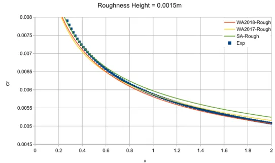
Figure 3.2 shows the comparison of computed results obtained by WA2018-Rough model,
WA2017-Rough model, SA-Rough model and Eq. (3.13). As the sand grain roughness height 𝑘𝑠
increases, the error in results obtained from each model increases. When 𝑘𝑠 is as small as 0.00025m, the flat plate has very small roughness, therefore the three turbulence models accurately predict the skin friction coefficient Cf. For 𝑘𝑠 = 0.0005m, the SA-Rough model’s predictions are more accurate compared to those from WA2017-Rough and WA2018-Rough
models at the leading edge, especially in the range 0 ≤ x ≤ 0.4m. When x > 0.4m, the two WA
19
shows the best agreement overall among the three models, while the SA-Rough model still has
the best agreement in a very limited range near the leading edge (x ≤ 0.4m). At this high level of
roughness, it is obvious that WA2017-Rough model cannot have the same result as
WA2018-Rough model in the range x ≤ 0.4m, but the two WA-Rough models are still much better overall
than the SA-Rough model. For 𝑘𝑠 = 0.0015m, WA2018-Rough model gives good result near
the leading edge, and has the best agreement near the trailing edge of the flat plate. The overall results from WA2018-Rough model are most accurate compared to the results from WA2017-Rough and SA-WA2017-Rough models.
20
Figure 3.2 (b) Comparison of 𝑪𝒇 for 𝒌𝒔= 𝟎. 𝟎𝟎𝟎𝟓 m.
21
Figure 3.2 (d) Comparison 𝑪𝒇 for 𝒌𝒔= 𝟎. 𝟎𝟎𝟏𝟓 m.
Figure 3.2 Comparison of 𝑪𝒇 for three turbulence models with roughness.
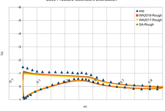
3.2.3 Flow past a 2D Rough S809 Airfoil
The second validation case is that of flow over a rough S809 airfoil, which is commonly used on wind turbine blades. The working environment for a wind turbine may be harsh, and as a consequence the surface of the turbine blades may become rough due to erosion, sand grits and cavitation. The computation results are compared using the SA-Rough model, WA2018-Rough model, and WA2017-Rough model are compared with the experimental data collected by Ramsay of Ohio State University [11]. In this case, the chord length Reynolds number is 1 million. Based on Ramsay’s work, the standard #40 lapidary grit is chosen to obtain a
relationship between the roughness height and chord length of ks/c=0.0019. Figure 3.3 shows the
comparison of pressure coefficient between experimental and computational data. The results using the three turbulence models depict very similar behavior for pressure coefficient prediction,
22
showing a very small drop in Cp at the leading edge which may be improved by using a finer mesh or a better-defined geometry of S809 airfoil.
Figure 3.3 Comparison of computed and experimental Cp on rough S809 airfoil at α=6.1°.
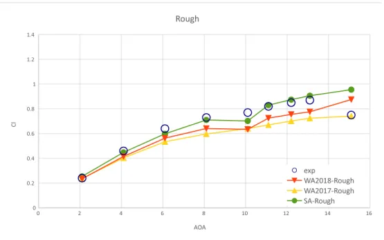
Figure 3.4 shows the variation in computed lift coefficient with angle of attack for a smooth S809 airfoil and its comparison with experimental data. The results in Figure 3.4 are quite reasonable since all the three models show a quasi-linear relationship between the angle of attack (AOA) and lift coefficient when AOA is below 10°. White [12] has stated that an airfoil will have a stall when the AOA is about 10° when the flow separation may occur, and the theory fails to predict the lift coefficient. Figure 3.5 shows the variation in computed lift coefficient with angle of attack for a rough S809 airfoil and its comparison with experimental data. It can be seen that both WA2017-Rough and WA2018-Rough model fail to predict the experimental data while the SA-Rough model performs reasonably well. According to Wray and Agarwal [9], the WA model also require a laminar-turbulent transition model to accurately predict the Cl for AOA > 8°.
23
The overall performance of the three models for rough S809 case is not as good as for the smooth S809.
Figure 3.4 Comparison of computations with three turbulence models and experimental data for smooth S809 airfoil.
24
3.2.4 Flow in a 2D Rough Wall Channel
The last validation case is the turbulent flow in a 2D rough-wall channel. The computational results from SA-Rough and WA2018-Rough models are compared to the experimental data collected by Saleh [13]. The channel has a cross section of 600*50 mm and a length of 2m. The channel cross section has an aspect ratio of 12.6:1 to ensure the two-dimensionality of the flow at the middle cross-section along the width of 600mm. Top and bottom surfaces of the channel are roughened by emery papers which have an average roughness height of 0.00125m. The computations are performed at two different inlet velocities which correspond to Reynolds numbers of 32,322 and 46,613 based on the channel height.
Figures 3.6 and 3.7 show the comparison of computed results and experimental data for fully developed turbulent flow in the channel at two different Reynolds numbers. WA2018-Rough model has overall better agreement with the experimental data than WA2017-Rough and SA-Rough model. The WA2018-SA-Rough model matches the experimental data more closely in the region near the centerline of the channel. In the near wall region, WA2017-Rough and SA-Rough model under-predict the velocity compared to WA2018-SA-Rough model; however all three models fail to match the experimental data.
25
Figure 3.6 Comparison of computed and experimental velocity profiles for fully developed turbulent flow in a rough channel at Re = 32,322.
Figure 3.7 Comparison of computed and experimental velocity profiles for fully developed turbulent flow in a rough channel at Re = 46,613.
26
Chapter 4: Development of a One-Equation
Algebraic Reynolds Stress Model based on k-kL
Closure
4.1 Introduction
The current version of two-equation k-kL model in the literature utilizes Abdol-Hamid’s closure based on Menter’s modification to Rotta’s two-equation model [14]. Rotta’s formulation
shows that the higher order velocity derivatives in the source terms in kL equation improve the
accuracy of simulation of unsteady flows, which is an important feature of this model [15]. Beyond the Boussinesq approximation for eddy-viscosity, Abdol-Hamid’s work shows that using an Algebraic Reynolds Stress Model (ARSM) to determine the Reynolds stress tensor would further improve the computational results for separated and corner flows [16].
In the present work, the one equation ARSM is derived from the two-equation k-kL-ARSM model of Abdol-Hamid [16] by employing additional assumptions by Bradshaw et al. [17] and Townsend [18]. The derived model is validated by several benchmark incompressible flow cases listed on NASA Turbulence Modeling Recourse (TMR) website. Computational results are compared with experimental data and other one-equation models. The proposed one-equation k-kL-ARSM model is employed to simulate flow past a flat plate, flow in 2D channel, flow over a 2D hump, flow past a backward-facing step, and flow in an asymmetric plane diffuser. The proposed one-equation k-kL-ARSM model shows good agreements with the experimental data, and it is even better in some cases compared to the SA and WA models.
27
4.2 The k-kL-ARSM Model
The one equation k-kL-ARSM is derived from Abdol-Hamid’s two equation k-kL-ARSM turbulence model [16]. To simplify the derivation process, the equations start with the boundary layer coordinates (x-streamwise coordinate, y- normal to the boundary layer) and the complete form of the model is given at the end of this section. The two-equation k-kL model in boundary layer coordinates can be written as:
𝐷𝑘 𝐷𝑡 = 𝐺 − 𝐶𝜇 3 4k 5 2 𝑘𝐿 − 1.5𝜐 𝑘 𝑑2+ 𝜕 𝜕𝑦((𝜈 + 𝜎𝑘𝜈𝑡) 𝜕𝑘 𝜕𝑦) (4.1) 𝐷(𝑘𝐿) 𝐷𝑡 = 𝐶𝜙1𝐺𝜙 𝑘𝐿 𝑘 − 𝐶𝜙2𝑘 3 2− 6𝑓𝜙𝜐𝑘𝐿 𝑑2 + 𝜕 𝜕𝑦((𝜈 + 𝜎𝜙𝜈𝑡) 𝜕𝑘𝐿 𝜕𝑦) (4.2)
where G and 𝐺𝜙 are the production terms for k and kL, respectively. Unlike the original k-kL model, the production terms 𝑃𝑘 and 𝑃𝑘𝐿 here are different. The production term, 𝑃𝑘𝐿 is limited by strain rate, S, and linear turbulence viscosity 𝜇𝑡𝐿 as described below:
𝐺 =𝜏𝑖𝑗 𝜌 𝜕𝑢𝑖 𝜕𝑦 (4.3) 𝐺∅ = 𝑃𝑘𝐿 𝜌 = max(𝐺, 𝜈𝑡 𝐿𝑆2) = max (𝐺, −𝑎1 2𝜈 𝑡𝑆2 𝛼 ) (4.4) 𝑆𝑖𝑗 = 1 2( 𝜕𝑢𝑖 𝜕𝑦 + 𝜕𝑢𝑗 𝜕𝑥) (4.5)
The turbulent viscosity is given by:
𝜈𝑡 = − 𝛼 𝐶𝜇 3 4 𝑘𝐿 𝑘12 (4.6)
To derive the one-equation k-kL model, we can express the time derivative of the eddy viscosity in terms of the time derivative of k and kL as:
28 𝐷𝜈𝑡 𝐷𝑡 = − 𝑎1 𝑆 ( 𝛼𝑆12 𝑎12𝜈 𝑡 1 2 𝐷(𝑘𝐿) 𝐷𝑡 − 1 2 𝐷𝑘 𝐷𝑡) (4.7)
To obtain a transport equation with only one independent scalar value, one more relation among 𝜈𝑡, 𝑘𝐿 and 𝑘 is required. The relationship is based on lot of experimental data and has been proposed by Bradshaw et al. [17] and Townsend [18] as:
𝜈𝑡| 𝜕𝑢
𝜕𝑦| = 𝐶𝜇
1
2𝑘 (4.8)
In general, the absolute value of streamwise velocity gradient along the normal direction |𝜕𝑢
𝜕𝑦| can be replaced by an invariant value S [19], and the value of 𝜕𝑣
𝜕𝑥 can be neglected.
|𝜕𝑢
𝜕𝑦| → 𝑆 (4.9)
Hence, k can be expressed as:
𝑘 =𝜈𝑡𝑆
𝑎1 (4.10)
and kL is given by:
𝑘𝐿 = −𝑎1𝜈𝑡
3 2𝑆12
𝛼 (4.11)
By combining Eq. (4.7) with Eqs. (4.1), (4.2), (4.6), (4.8) and (4.9), the one-equation k-kL-ARSM model can be derived as:
𝐷𝜈𝑡 𝐷𝑡 = (𝐶𝜙1𝐺∅− 𝐺 2 ) 𝑎1 𝑆 + ( 𝐶𝜙2 𝑎15/2 − 1 2𝑎1 ) 𝛼 𝜈𝑡𝑆 + 𝜈𝜈𝑡(34− 6𝑓𝜙) 𝑑2 + (2𝜎𝜙− 3 2𝜎𝑘) 𝜈𝑡 𝑆 𝜕𝜈𝑡 𝜕𝑥𝑖 𝜕𝑆 𝜕𝑥𝑖 + (9 4𝜎𝜙− 1 2𝜎𝑘) 𝜕𝜈𝑡 𝜕𝑥𝑖 𝜕𝜈𝑡 𝜕𝑥𝑖 + (3 2𝜎𝜙− 1 2𝜎𝑘) 𝜈𝑡 𝜕2𝜈 𝑡 𝜕𝑦2 + ( 1 2𝜎𝜙− 1 2𝜎𝑘) 𝜈𝑡 2 2 𝑆−1𝜕 2𝑆 𝜕𝑦2 +2𝜎𝜙𝜈𝑡 2 𝛼2 𝜕𝛼 𝜕𝑥𝑖 𝜕𝛼 𝜕𝑥𝑖 −𝜎𝜙𝜈𝑡 2 4𝑆2 𝜕𝑆 𝜕𝑥𝑖 𝜕𝑆 𝜕𝑥𝑖 −4𝜎∅𝜈𝑡 𝛼 𝜕𝛼 𝜕𝑥𝑖 𝜕𝜈𝑡 𝜕𝑥𝑖 −𝜎𝜙𝜈𝑡 2 𝛼𝑆 𝜕𝛼 𝜕𝑥𝑖 𝜕𝑆 𝜕𝑥𝑖 −𝜎𝜙𝜈𝑡 2 𝛼 𝜕2𝛼 𝜕𝑦2 (4.12)
29
The diffusive coefficients in k and kL equations are assumed to be equal, and this assumption
helps us to simplify and calibrate the coefficient of the one-equation k-kL-ARSM model. The diffusive coefficients are calibrated as follows:
𝜎𝜙 = 𝜎𝑘 = 𝜎 = 0.7 (4.13)
In addition, to avoid singularity in the von Karman length-scale when 𝑆 → 0, especially for channel flow near the centerline region where S will be extremely small, and to ensure convergence, Eq. (4.12) can be rewritten as:
𝐷𝜈𝑡 𝐷𝑡 = (𝐶𝜙1𝐺∅1− 1 2𝐺) 𝑎1 𝑆 + ( 𝐶𝜙2 𝑎15/2− 1 2𝑎1 −1) 𝛼𝜈 𝑡𝑆 + 𝜈𝜈𝑡(34−6𝑓𝜙) 𝑑2 + 𝜎𝜈𝑡 2𝑆 𝜕𝜈𝑡 𝜕𝑥𝑖 𝜕𝑆 𝜕𝑥𝑖+ 3𝜎 4 𝜕𝜈𝑡 𝜕𝑥𝑖 𝜕𝜈𝑡 𝜕𝑥𝑖+ 2𝜎𝐶4𝐸𝐵𝐵tanh ( 𝐸𝑘𝛼 𝐶4𝐸𝐵𝐵) − 4𝜎𝜈𝑡 𝛼 𝜕𝛼 𝜕𝑥𝑖 𝜕𝜈𝑡 𝜕𝑥𝑖− 𝜎𝜈𝑡2 𝛼𝑆 𝜕𝛼 𝜕𝑥𝑖 𝜕𝑆 𝜕𝑥𝑖− 𝜎𝜈𝑡2 𝛼 𝜕2𝛼 𝜕𝑥𝑖2− 1 4𝜎𝐶3𝐸𝐵𝐵tanh ( 𝐸𝑘𝑘𝑙 𝐶3𝐸𝐵𝐵) + 𝜕 𝜕𝑥𝑗((𝜎𝜈𝑡+ 𝜈) 𝜕𝜈𝑡 𝜕𝑥𝑗) (4.14) where 𝐶𝜙1 = (𝜁1− 𝜁2(−𝐶𝜇√𝜈𝑡 𝛼√𝑆𝐿𝑣𝑘 ) 2 ) 𝐶𝜙2= 𝜁3 𝑓𝜙 =1 + 𝐶𝑑1𝜉 1 + 𝜉4 𝐿𝑣𝑘 = 𝜅 |𝑈′ 𝑈′′| 𝑈′= √2𝑆𝑖𝑗𝑆𝑖𝑗 𝑈′′ = √(𝜕 2𝑢 𝜕𝑥2+ 𝜕2𝑢 𝜕𝑦2+ 𝜕2𝑢 𝜕𝑧2)2+ ( 𝜕2𝑣 𝜕𝑥2+ 𝜕2𝑣 𝜕𝑦2+ 𝜕2𝑣 𝜕𝑧2)2+( 𝜕2𝑤 𝜕𝑥2 + 𝜕2𝑤 𝜕𝑦2 + 𝜕2𝑤 𝜕𝑧2)2 𝜉 = 𝑑√0.3𝜈𝑎𝑡𝑆 1 20𝜈
30 𝐸𝐵𝐵 = 𝜕𝜈𝑡 𝜕𝑥𝑖 𝜕𝜈𝑡 𝜕𝑥𝑖 𝐸𝑘𝛼 = 𝜕𝛼 𝜕𝑥𝑖 𝜕𝛼 𝜕𝑥𝑖 𝜈𝑡2 𝛼2 𝐸𝑘𝑘𝑙 = 𝜕𝑆 𝜕𝑥𝑖 𝜕𝑆 𝜕𝑥𝑖 𝜈𝑡2 𝑆2 The following limiter on 𝐿𝑣𝑘 is employed:
𝐿𝑣𝑘,𝑚𝑖𝑛≤ 𝐿𝑣𝑘 ≤ 𝐿𝑣𝑘,𝑚𝑎𝑥 where 𝐿𝑣𝑘,𝑚𝑖𝑛 = − 𝑎1 2𝜈 𝑡 1/2 𝐶11𝛼𝑆1/2 𝐿𝑣𝑘,𝑚𝑎𝑥 = 𝐶12𝜅𝑑𝑓𝑝 𝑓𝑝 = 𝑚𝑖𝑛 [𝑚𝑎𝑥 (− 𝐶𝑟1𝐺∅𝑎12 𝛼𝜈𝑡𝑆2 , 0.25) , 1.0]
The constants in the model are:
𝜁1 = 1.4 𝜁2 = 0.97 𝜁3 = 0.137 𝜅 = 0.41 𝑎1 = √𝐶µ = 0.3
𝐶11= 10.0 𝐶12= 1.3 𝐶𝑑1 = 4.7 𝐶3 = 𝐶4 = 7.0 𝜎 = 0.7 𝐶𝑟1 = 0.5 Instead of using the Boussinesq assumption, the turbulent stress term is given by:
𝜏𝑖𝑗 = 𝜏𝑖𝑗𝐴𝑅𝑆𝑀 = −𝜌𝑘 [∑ 𝑎𝑖𝑗 +2
3𝛿𝑖𝑗] = −𝜌𝑘 [∑ 𝛽𝜆𝑇
(𝜆)+2
3𝛿𝑖𝑗] (4.15)
where 𝑇(𝜆) is a group of second order tensors that are function of strain and vorticity rates, S and
W, respectively. 𝑎𝑖𝑗 is a symmetric traceless second order tensor, which is dependent on 𝑇(𝜆):
𝑇(1)= [𝑆∗−1 3𝑡𝑟{𝑆 ∗}𝐼], 𝑇(2)= [𝑆∗2−1 3𝑡𝑟{𝑆 ∗2}𝐼] 𝑇(3)= [𝑊∗2−1 3𝑡𝑟{𝑊 ∗2}𝐼], 𝑇(4)= [𝑆∗𝑊∗− 𝑊∗𝑆∗]
31 𝑇(5)= [𝑆∗2𝑊∗− 𝑊∗𝑆∗2], 𝑇(6)= [𝑆∗𝑊∗2− 𝑊∗2𝑆∗−2 3𝑡𝑟{𝑆 ∗𝑊∗2}𝐼] 𝑇(7)= [𝑆∗2𝑊∗2+ 𝑊∗2𝑆∗2−2 3𝑡𝑟{𝑆 ∗2𝑊∗2}𝐼] , 𝑇(8)= [𝑊∗𝑆∗𝑊∗2− 𝑊∗2𝑆∗𝑊∗] 𝑇(9)= [𝑊∗𝑆∗𝑊∗2− 𝑊∗2𝑆∗𝑊∗], 𝑇(10)= [𝑊∗𝑆∗2𝑊∗2− 𝑊∗2𝑆∗2𝑊∗]
The k-kL-ARSM model utilizes three tensors of 𝑇(𝜆)(𝜆 = 1, 2, 𝑎𝑛𝑑 4) as follows:
𝜏𝑖𝑗𝐴𝑅𝑆𝑀 = −𝜌𝑘 (𝛽1𝑇(1)+ 𝛽2𝑇(2)+ 𝛽4𝑇(4)+2
3𝛿𝑖𝑗) (4.16)
where 𝑇(1) is the linear part of the model, and 𝑇(2) and 𝑇(4) are the nonlinear anisotropic terms. I is the identity matrix. The 𝛽𝜆 coefficients are:
𝛽1= −2𝐶𝜇∗ = 2𝛼, 𝛽2 = −2𝑎4𝑎3𝛽1, 𝛽4 = 𝑎4𝑎2𝛽1
In the model, 𝐶𝜇∗ is limited to be no smaller than 0.0005. 𝛼 is the root of the cubic equation:
𝛼3+ 𝑝𝛼2+ 𝑞𝛼 + 𝑟 = 0 (4.17)
where coefficients in 𝑇(𝜆) are:
𝑎1 = 1 2( 4 3− 𝐶2) , 𝑎2 = 1 2(2 − 𝐶4) 𝑎3 = 1 2(2 − 𝐶3), 𝑎4 = [𝛾1 ∗− 2𝛼𝛾 0∗𝜂2]−1
The following definitions and constants are also used. Note that the coefficient 𝑎1 above is the coefficient in 𝑇(𝜆) and is not computed from √𝐶
µ. 𝜏 = −1.51𝑎1 𝛼𝑆 𝑊𝑖𝑗∗ = 𝜏𝑊𝑖𝑗, 𝑆𝑖𝑗∗ = 𝜏𝑆𝑖𝑗 𝜂2 = {𝑆∗2}, 𝛾 0∗ = 𝐶11 2 , 𝛾1 ∗ =𝐶1 0 2 + 𝐶𝜀2− 𝐶𝜀1 𝐶𝜀1− 1 𝐶𝜀1= 1.44, 𝐶𝜀2= 1.83 𝐶11 = 1.8, 𝐶10 = 3.4
32 𝐶2 = 0.36, 𝐶3 = 1.25, 𝐶4 = 0.6 𝑝 = − 𝛾1 ∗ 𝜂2𝛾 0∗ 𝑞 = 1 (2𝜂2𝛾 0∗)2 (𝛾1∗2− 2𝜂2𝛾0∗𝑎1− 2 3𝜂 2𝑎 32− 2𝑅2𝜂2𝑎22) 𝑟 = 𝛾1 ∗𝑎 1 (2𝜂2𝛾 0∗)2 {𝑊∗2} = −𝑊 𝑖𝑗∗𝑊𝑖𝑗∗, 𝑅2 = − {𝑊∗2} {𝑆∗2}
The root with the lowest real part was chosen from this cubic equation. If 𝜂2 < 10−6, then
𝛼 = − 𝛾1 ∗𝑎 1 𝛾1∗2− 2{𝑊∗2}𝑎 2 2 Otherwise, define: 𝑎 = 𝑞 −𝑝 2 3 , 𝑏 = 1 27(2𝑝 3− 9𝑝𝑞 + 27𝑟), 𝑑 = 𝑏2 4 + 𝑎3 27 If d > 0, 𝑡1 = (−𝑏 2+ √𝑑) 1 3 , 𝑡1 = (−𝑏 2− √𝑑) 1 3 𝛼 = min (−𝑝 3+ 𝑡1+ 𝑡2, − 𝑝 3− 𝑡1 2 − 𝑡2 2) else if d ≤ 0, 𝜃 = cos−1 ( − 𝑏 2√−27)𝑎3 𝛼 = min (𝑡1, 𝑡2, 𝑡3) where
33 𝑡1 = −𝑝 3+ 2√− 𝑎 3cos ( 𝜃 3) 𝑡2 = −𝑝 3+ 2√− 𝑎 3cos ( 2𝜋 3 + 𝜃 3) 𝑡3 = −𝑝 3+ 2√− 𝑎 3cos ( 4𝜋 3 + 𝜃 3)
Note that all the terms having k and kL in the original two-equation k-kL-ARSM model are replaced by using Eq. (4.10) and (4.11).
The boundary conditions at the wall is
(𝜈𝑡)𝑤𝑎𝑙𝑙 = 0
In the far field region, boundary condition is recommended to be: (𝜈𝑡)𝑓𝑎𝑟𝑓𝑖𝑒𝑙𝑑 = 3𝜈∞: 𝜈𝑡: 5𝜈∞
4.3 Validation Cases
The one-equation k-kL-ARSM was validated by computing several benchmark test cases on NASA TMR’s website which include flow past a flat plate, flow in a 2D channel, flow over a 2D hump, flow past a backward-facing step, flow past a curved backward-facing step, flow in an asymmetric plane diffuser and supersonic flow in a square duct. The computational results are compared with the model predictions from one-equation k-kL, WA2018 and SA models, available DNS results or experimental data for each case.
4.3.1 Zero Pressure Gradient Boundary-Layer Flow Past a Flat Plate
A low-speed zero pressure gradient turbulent flow past a flat plate is the first and foremost case need to validate a turbulence model. The experimental results are given by Wieghardt and
34
Tillman [20]. A uniform inlet velocity of Uin=68.6m/s (based on flow parameters in Figure 4.1)
was used as fully turbulent inlet flow condition.
Figure 4.1Boundary conditions for the flat plate case [1].
Figure. 4.2 shows the skin friction coefficient Cf computed using the one-equation k-kL-ARSM model, SA model and experimental data. The Reynolds number in x direction Rex, is computed form Eq. (4.18):
Rex= 𝑈∞x
𝜈∞ (4.18)
In the region when Rex is less than approximate 5 million, it is obvious that the one-equation
k-kL-ARSM has the best agreement with the experimental data. The overall performance of four turbulence models are reasonably good and close as expected.
35
Figure 4.2 Skin friction vs. Rex for turbulent boundary layer flow past a flat plate.
4.3.2 Flow in a 2D Channel at Different Reynolds Numbers
Another basic validation case is the fully developed turbulent channel flow. For the channel flow, three friction Reynolds numbers of 182, 1000 and 5200 were selected to validate the one-equation k-kL-ARSM model. Fully developed velocity profiles were compared with SA, WA2018 and one-equation k-kL models and the DNS data by Lee and Moser [21]. Figures. 4.3-4.8 show the fully developed velocity profiles and near wall velocity profiles for friction Reynolds numbers of 182, 1000, and 5200, respectively. Overall, the four models have good agreement with the DNS data. It is obvious that the SA model has the best results for the near wall velocity profiles, especially in the log layer. The one-equation k-kL-ARSM has reasonably good results for fully developed velocity profile in large y+ region. It is better than the
one-equation k-kL model when Reτis small. However, with increasing friction Reynolds number, the
one-equation k-kL model has better results than WA2018 and the k-kL-ARSM model. The new k-kL-ARSM model may need to include an extra elliptic partial differential equation, which is also known as elliptic relaxation, to improve the near wall velocity profile in log layer [22].
36
Excellent improvement in the near wall region velocity profile using elliptic blending has been shown by several researchers.
Figure 4.3 Near wall velocity profile in the channel at Reτ = 182.
37
Figure 4.5 Near Wall velocity profile in the channel at Reτ = 1000.
38
Figure 4.7 Near Wall velocity profile in the channel at Reτ = 5200.
Figure 4.8 Velocity profile in the channel at Reτ = 5200.
An additional channel flow at high Reynolds number was also computed (as suggested on NASA TMR) to test the new model with inflow Mach number of 0.2 and Reynolds number of 80 million based on channel height. The velocity profile from the new k-kL-ARSM model is
39
compared to that obtained from SA model at x=500. Figure 4.9 shows that the new one-equation k-kL-ARSM model agrees well with SA model for the velocity profile.
Figure 4.10 shows the comparison of the turbulent viscosity ratio (𝜇𝑡/𝜇). The WA model has
an obvious the best profile among the four models; the other models have “kinks” near the centerline region. It can be seen from this figure that the two k-kL models have very similar “kinks”, which indicate that the models cannot properly handle the sudden drop in the shear strain rate S near centerline. Hence, the conversion of the term 𝜎𝜙𝜈𝑡2
4𝑆2
𝜕𝑆 𝜕𝑥𝑖
𝜕𝑆
𝜕𝑥𝑖 in Eq. (4.12) may not be
enough, and further correction may be needed to fix the “kink.”
40
Figure. 4.10 Comparison of turbulent viscosity ratio in fully developed turbulent channel flow, 𝑹𝒆𝒉= 𝟖𝟎 × 𝟏𝟎𝟔.
4.3.3 Flow past 2D NASA Wall-Mounted Humps
Due to the insensitivity to Reynolds number and response to active flow control, flow over a wall-mounted hump is a classical flow separation case which has been extensively computed for validating various turbulence models. The geometry and boundary conditions of experimental flow are shown in Figure. 4.11, which are given by Seifert and Pack [23] and Greenblatt et al.
[24]. Due to freestream Ma=0.1, and Rec=936,000 based on hump chord length, a fully turbulent
flow condition is used with a uniform inlet velocity of Uinlet=34.6m/s. The calculation of skin friction coefficient and pressure coefficient are of interest in this case.
41
The comparison of skin friction coefficient Cf is shown in Figure. 4.12. Before the flow
separation, the one-equation k-kL model obviously fails to predict the magnitude of Cf along the
hump wall. On the other hand, the new k-kL-ARSM model has the best result in the region near the separation point, and the WA2018 underpredicts the magnitude of Cf in this region. The kinks in the result from the four models may be caused by mesh near the wall, and it should be eliminated by a set of finer grids. The flow separation occurs at location x/c=0.6~0.7; all four models have overall good agreement with the experimental data, however the SA model underpredicts the value of Cf at the location x/c ≈ 0.6. The one-equation k-kL-ARSM gives a
good prediction of the reattachment point near x/c=1.0 and the Cf between separation point and
reattachment point is identical to the experimental data and SA model. On the other hand, WA2018 and one-equation k-kL fail to predict the Cf in this region accurately. For the region
x/c >1, it is obvious that the newly proposed k-kL-ARSM model has Cf, which is much closer to
the experimental data.
42
Figure 4.13 shows the comparison of pressure coefficient Cp. The new k-kL-ARSM model and SA model have identical results which overlap each other. The one-equation k-kL model is most accurate while WA2018 is relatively not that accurate.
In this case, the new one-equation k-kL-ARSM has successfully predicted the flow separation and reattachment. The overall performance of the new model in prediction of Cf and Cp is the best among the four models.
Figure 4.13 Comparison of pressure coefficient for flow over a 2D hump.
4.3.4 Flow over a 2D Backward-Facing Step
The 2D backward-facing step is a typical benchmark case for computation of separated flow. In this case, flow separation is induced by a turbulent boundary layer encountering a sudden back step. The experimental data has been obtained by Driver and Seegmillar [25]. The step has a
height of H=0.0127m. Hence, the Reynolds number Re based on the step height is 3.6×10⁴, and
the Mach number Ma is 0.128 at the reference point (x/H=-4). The fully turbulent boundary conditions are used in this case; the details of the boundary conditions and geometry are given in Figure 4.14.
43
Figure 4.14 Backward facing step geometry and flow conditions [1].
The comparison of skin friction coefficient at the bottom wall is shown in Figure 4.15. One of the key measures of success is the capability to predict the reattachment point. The experimental data shows that the reattachment point is at about x/H=6.3, which is accurately predicted by all the models. Even though SA model is more accurate at upstream of the step, the one-equation k-kL-ARSM performs better all the way down to the outlet of the channel. Moreover, the one-equation k-kL model is slightly better than the k-kL-ARSM model after the reattachment point. The WA2018 has the best agreement with the experimental data.
44
Figure 4.16 shows the comparison of pressure coefficients at the step wall. All the models fail
to predict accurately the magnitude of Cp at the beginning of the separation region, however the
one-equation k-kL model has the almost identical results as the experimental data near the reattachment point in the separation region. WA2018 model predicts a delayed reattachment point compared to the experimental data. Except for WA2018, the pressure coefficients shown in Figure 4.16 are consistent with the results in Figure 4.15 for the prediction of the reattachment
point. For Cp in Figure 4.16, even though the one-equation k-kL is the most accurate model, the
new k-kL-ARSM is reasonably good with acceptable error.
Figure 4.16 Pressure coefficients along the step wall of the backward facing step.
4.3.5 Flow over a 2D Curved Backward-Facing Step
Another flow separation case is the flow over a curved backward-facing step, which is more complex than the previous backward-facing step case. The Reynolds number based on step height and inlet velocity is 13,700. The validation data is from LES by Bentaleb et al [26].
As shown in Figure 4.17, for Cf, the flow separates at x/H=0.83 and reattaches at x/H = 4.36.
(x/H=0-45
0.83), the one-equation k-kL-ARSM and one-equation k-kL models give the best agreement with the LES data. The new k-kL-ARSM model has identical result as the LES data after the separation point (x/H≈0.83-2.8) but has slightly delayed prediction of the separation location. All four models fail to accurately predict the reattachment point. Right after the flow reattachment, WA2018 and SA models have similar and better results than the k-kL, k-kL-ARSM models. However, both the k-kL and k-kL-k-kL-ARSM models have very good agreement with the LES data downstream (x/H>6).
Figure 4.17 Skin friction coefficients along the lower wall of the curved backward facing step.
The comparison of pressure coefficient is shown in Figure 4.18. The one-equation k-kL-ARSM model shows the best result among the four models. The significant difference occurs in the separation and reattachment regions. This case shows that the algebraic Reynolds-Stress model (ARSM) can improve the performance when computing a separated flow.
46
Figure 4.18 Pressure coefficients along the step wall of the curved backward facing step.
4.3.6 Flow in a 2D Asymmetric Plane Diffuser
Figure 4.19 shows the computational geometry of the asymmetric plane diffuser. It is the Buice and Eaton asymmetric diffuser study #1 (baseline) from NPARC Alliance CFD Verification and Validation Archive [27]. Based on Buice and Eaton’s work [28], the Reynolds number Re based on the width of the inflow is 20,000, and inlet Mach number Ma is 0.06. The flow separation occurs at the inclined wall due to the adverse pressure gradient. It is a challenging case to predict accurately by the turbulence models. The quantities of interests in this case are skin friction coefficient and pressure coefficient along the lower wall and the upper wall of the diffuser.
47
Figure 4.19 Geometry of the 2D asymmetric plane diffuser [27].
Figures 4.20 and 4.21 show the comparison of skin friction coefficient on the bottom wall and top wall, respectively. It can be seen from Figure 4.20 that the experimental data indicates the flow separates at x/h≈7.6 and reattaches at x/h≈28.0 along the bottom wall. In this case, the one-equation k-kL model fails to predict either the separation point or the reattachment point, as well as the behavior in the separation bubble as shown in Figure 4.24. The SA and new k-kL-ARSM model give an early prediction of the separation point; however WA2018 model shows the ability to accurately predict the separation. Considering the downstream region, the one-equation k-kL-ARSM is the only model that has good agreement with the experimental data near the reattachment region and after-reattachmen
![Figure 3.1 Flat plate geometry and boundary conditions [1].](https://thumb-us.123doks.com/thumbv2/123dok_us/275182.2528287/32.918.248.725.105.369/figure-flat-plate-geometry-boundary-conditions.webp)

![Figure 4.1 Boundary conditions for the flat plate case [1].](https://thumb-us.123doks.com/thumbv2/123dok_us/275182.2528287/48.918.240.703.188.424/figure-boundary-conditions-flat-plate-case.webp)


