January 2005, Volume 12, Issue 6. http://www.jstatsoft.org/
spatstat: An
R
Package for Analyzing Spatial Point
Patterns
Adrian BaddeleyUniversity of Western Australia
Rolf Turner
University of New Brunswick
Abstract
spatstatis a package for analyzing spatial point pattern data. Its functionality includes exploratory data analysis, model-fitting, and simulation. It is designed to handle realistic datasets, including inhomogeneous point patterns, spatial sampling regions of arbitrary shape, extra covariate data, and ‘marks’ attached to the points of the point pattern.
A unique feature of spatstat is its generic algorithm for fitting point process models to point pattern data. The interface to this algorithm is a function ppmthat is strongly analogous to lmandglm.
This paper is a general description ofspatstatand an introduction for new users.
Keywords: conditional intensity, edge corrections, exploratory data analysis, generalised linear models, inhomogeneous point patterns, marked point patterns, maximum pseudolikeli-hood, spatial clustering .
1. Introduction
spatstat is one of several packages in the R language for analysing point patterns in two
dimensions. 1 This paper is a general description ofspatstatand may serve as an introduction for new users. Subsequent papers will cover advanced use of the packageBaddeley and Turner
(2005b) and explain its design and implementationBaddeley and Turner(2005a).
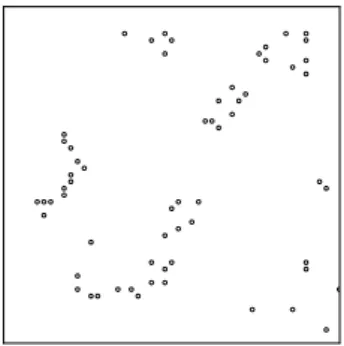
A simple example of a point pattern dataset is shown in Figure1. The points represent the locations of seedlings and saplings of the Californian giant redwood.
Point pattern data may be much more complicated than Figure 1 suggests. The spatial sampling region in which the points were recorded may have arbitrary irregular shape, instead of being a rectangle as in Figure 1. The points may carry additional data (marks). For example, we may have recorded the height or the species name of each tree. There may be
1
Alternatives includesplancsRowlingson and Diggle(1993);Bivand(2001),spatialRipley(2001);Venables and Ripley(1997),ptprocPeng(2003) andSSLibHarte(2003).
Figure 1: The classic Redwoods dataset Ripley(1977) available inspatstat asredwood.
additional covariate data which must be incorporated in the analysis. The spatstat package is designed to handle all these complications.
Figure2shows an example of a dataset which can be handled byspatstat; it consists of points of two types (plotted as two different symbols) and is observed within an irregular sampling region which has a hole in it. The label or ‘mark’ attached to each point may be a categorical variable, as in the Figure, or a continuous variable. See also Figures 6–9.
Figure 2: Artificial example demonstrating the complexity of datasets which spatstat can handle.
Point patterns analysed in spatstat may also be spatially inhomogeneous, and may exhibit dependence on covariates. The package can deal with a variety of covariate data structures. It will fit point process models which depend on the covariates in a general way, and can also simulate such models.
2. Goals
Our main reasons for writingspatstatwere to:Implement functionality. The research literature on spatial statistics provides a large body of techniques for analysing spatial point patterns (e.g. Bartlett (1975); Cliff and Ord
(1981); Cressie (1991); Diggle (2003); van Lieshout (2000); Mat´ern (1986); Møller and
Waagepetersen(2003);Moore (2001);Ripley(1981,1988);Stoyan, Kendall, and Mecke
(1995);Stoyan and Stoyan(1995);Upton and Fingleton(1985)). However, only a small
Handle real datasets. New techniques published in the literature are often demonstrated only on a ‘tame’ example dataset, using a rudimentary proof-of-concept implementa-tion. Such software is typically designed only for rectangular windows; the techniques themselves may assume that the point pattern is spatially homogeneous; and auxiliary information (such as covariate data) is often ignored.
For example, the classical redwood dataset of Figure 1 is a subset extracted byRipley
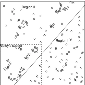
(1976, 1981) from a larger dataset of Strauss (1975) which is shown in Figure 3. The full dataset exhibits completely different spatial patterns on either side of the diagonal line shown on the plot. The diagonal line is a simple example of covariate data. As far as we are aware, the full dataset has never been subjected to comprehensive analysis.
Strauss’s redwood data
Region I Region II
Ripley’s subset
Figure 3: The full redwood dataset of Strauss (1975). The square in the bottom left corner shows the boundaries of the subset extracted byRipley(1977) as the classicalredwooddataset. Similarly, Figure 4 shows the ant nest data of Harkness and Isham (1983). The full dataset records the locations of nests of two species of ants, observed in an irregular convex polygonal boundary, together with annotations showing a foot track through the region, and the boundary between field and scrub areas inside the region. Rectangular subsets of the data (marked “A” and “B” on the Figure) were analysed in Harkness and
Isham (1983); Isham(1984); Takacs and Fiksel(1986);H¨ogmander and S¨arkk¨a (1999);
Baddeley and Turner (2000) and (S¨arkk¨a 1993, section 5.3). Again, as far as we are
aware, the full dataset has never been subjected to detailed analysis inside the correct window.
Fit realistic models to data. In applications, the statistical analysis of spatial point pat-terns is conducted almost exclusively using ‘exploratory’ summary statistics such as the KfunctionCliff and Ord(1981);Cressie(1991);Diggle(2003);Møller and Waagepetersen
Fin-gleton (1985). An important goal of spatstat is to fit parametric models to spatial point pattern data. Although methods for fitting point process models have been avail-able since the 1970’s Besag (1975); Diggle (2003); Ogata and Tanemura (1981,1984);
Møller and Waagepetersen(2003);Ripley(1981,1988), most of these methods were very
specific to the chosen model, and there were no software implementations of sufficient generality to fit realistic models to a real dataset. Recently we described an algorithm for fitting point process models of very general form Baddeley and Turner(2000). Our implementation of this algorithm has grown into the package spatstat.
ants
A
B
Figure 4: Harkness-Isham ant nests data. Map of the locations of nests of two species of ants,
Messor wasmanni(4) andCataglyphis bicolor(
◦
) in an irregular region 425 feet in diameter. Data kindly supplied by Professors R.D. Harkness and V. Isham.3. Capabilities
spatstatsupports the following activities.
Creation, manipulation and plotting of point patterns: a point pattern dataset can easily be created, plotted, inspected, and transformed. Subsets of the pattern can easily be extracted (e.g. to thin the points or trim the window). Marks can readily be added or removed from a point pattern. Many geometrical transformations, operations and measurements are implemented.
Exploratory data analysis: standard empirical summaries of the data, such as the average intensity, the K function Ripley (1977) and the kernel-smoothed intensity map, can easily
be generated and displayed. Many other empirical statistics are implemented in the package, including the empty space functionF, nearest neighbour distance functionG, pair correlation function g, inhomogeneous K functionBaddeley, Møller, and Waagepetersen (2000), second moment measure, Bartlett spectrum, cross-K function, cross-G function, J-function, and mark correlation function. Our aim is eventually to implement the vast majority of the statistical techniques described in the spatial statistics literature (e.g. Diggle (2003);Stoyan
and Stoyan(1995)).
Parametric model-fitting: a key feature of spatstat is its generic algorithm for fitting point process models to data. The point process models to be fitted may be quite general Gibbs/Markov models; they may include inhomogeneous spatial trend, dependence on co-variates, and interpoint interactions of any order (i.e. not restricted to pairwise interactions). Models are specified using aformulain theRlanguage, and are fitted using a single function
ppmanalogous toglmandgam. A fitted model can be printed, plotted, predicted, updated, and simulated. Capabilities for residual analysis and model diagnostics will be added in version 1.6.
Simulation of point process models: spatstat can generate simulated realisations of a wide variety of stochastic point processes. Some process parameters (intensity function, cluster distribution) may be arbitrary, user-supplied functions in the R language. Markov point process models of a very general kind (including arbitrary spatial inhomogeneity and user-supplied interaction potential) are simulated using a fast Fortran implementation of the Metropolis-Hastings algorithm. Fitted model objects obtained from the model-fitting algorithm can be simulated directly by Metropolis-Hastings.
4. Demonstration
A few examples of spatstat’s capabilities are shown in the following transcript of an R ses-sion. A more extensive demonstration can be seen by installing the package and typing
demo(spatstat).
R> library(spatstat) R> data(cells)
R> cells
planar point pattern: 42 points window: rectangle = [0,1] x [0,1]
R> plot(cells)
R> plot(ksmooth.ppp(cells)) R> plot(Kest(cells))
These commands performed some exploratory analysis of the dataset cells. The last two lines displayed a kernel-smoothed estimate of the intensity, and an estimate of theKfunction.
R> fit <- ppm(cells, ~1, Strauss(r=0.1)) R> fit
Stationary Strauss process beta
290.4221
interaction distance: 0.1
Fitted interaction parameter gamma: [1] 0.0126
R> Xsim <- rmh(fit) R> plot(Xsim)
This code fits a Strauss point process model to thecellsdata. The objectfitis a fitted point process model. The code prints a summary of the fitted model, then simulates a realisation from this fitted model.
R> data(demopat)
R> plot(demopat, box=FALSE) R> plot(split(demopat))
R> plot(alltypes(demopat, "K"))
This code analyzes the point pattern shown in Figure2which consists of points of two different types. Thesplitcommand separates the dataset into two point patterns according to their types, which are then plotted separately. The alltypes command computes the bivariate (‘cross’) K function Kij(r) for each pair of types i, j and plots them as a 2×2 array of graphs.
R> pfit <- ppm(demopat, ~marks + polynom(x,y,2), Poisson()) R> plot(pfit)
The call to ppm fits a non-stationary Poisson point process to the data in Figure 2. The logarithm of the intensity function of the Poisson process is described by the R formula
~marks + polynom(x,y,2) which represents a log-quadratic function of the cartesian
coor-dinates, multiplied by a constant factor depending on the type of point. The last line plots the fitted intensity function as a perspective view of a surface.
5. Data types
The basic data types in spatstat are Point Patterns, Windows, and Pixel Images. A point pattern is a dataset recording the spatial locations of all ‘events’ or ‘individuals’ observed in a certain region. A window is a region in two-dimensional space. It usually represents the ‘study area’. A pixel image is an array of “brightness” values for each grid point in a rectangular grid inside a certain region. It may contain covariate data (such as a satellite image) or it may be the result of calculations (such as kernel smoothing).
x
Figure 5: A point pattern, a window, and a pixel image.
spatstat uses the object-oriented features of R (“classes and methods”) to make it easy to
manipulate, analyse, and plot these datasets.
Note that there is no predetermined format for covariate data. Indeed that would be un-necessarily limiting, as there are many different kinds and formats of covariate information that might be needed. Our modelling and simulation code accepts covariate data in various formats.
5.1. Point patterns
A point pattern is represented inspatstat by an object of the class "ppp". A dataset in this format contains the coordinates of the points, optional ‘mark’ values attached to the points, and a description of the spatial region or ‘window’ in which the pattern was observed. To create a point pattern (class "ppp") object we may create one from raw data using the functionppp, convert data from other formats (including other packages) usingas.ppp, read data from a file using scanpp, manipulate existing point pattern objects using a variety of tools, or generate a random pattern using one of the simulation routines.
For example, to create a pattern of random points inside the rectangle [0,10]×[0,3], R> x <- runif(20, max=10)
R> y <- runif(20, max=3)
R> u <- ppp(x, y, c(0,10), c(0,3))
The Venables and Ripley spatial library, which is part of the standard distribution of R, supplies a datasetpines. To convert this into our format,
R> library(spatial)
R> pines <- ppinit("pines.dat") R> library(spatstat)
R> pines <- as.ppp(pines)
A point pattern must have a window
Note especially that, when you create a new point pattern object, you need to specify the spatial region or window in which the pattern was observed.
We believe that the observation window is an integral part of the point pattern. A point pattern dataset consists of knowledge about where points were not observed, as well as the
locations where theywereobserved. Even something as simple as estimating the intensity of the pattern depends on the window of observation. It would be wrong, or at least different, to analyze a point pattern dataset by “guessing” the appropriate window (e.g. by computing the convex hull of the points). An analogy may be drawn with the difference between sequential experiments and experiments in which the sample size is fixed a priori.
For situations where the window is really unknown,spatstatprovides the functionriprasto compute the Ripley-Rasson estimator of the window, given only the point locations Ripley
and Rasson(1977).
Marked point patterns
Each point in a spatial point pattern may carry additional information called a ‘mark’. For example, a pattern of points which are classified into two or more different types (on/off, case/control, species, colour, etc) may be regarded as a pattern of marked points, where the mark attached to each point indicates which type it is. Data recording the locations and heights of trees in a forest can be regarded as a marked point pattern where the mark attached to a tree’s location is the height of the tree.
In our current implementation, the mark attached to each point must be asingle value (which may be numeric, character, complex, logical, or factor). Many of the functions inspatstatfor marked point patterns require that the mark attached to each point be either
• a continuous variate or “real number”. An example is the Longleaf Pines dataset
(longleaf) in which each tree is marked with its diameter at breast height. Themarks
component must be a numericvector such thatmarks[i]is the mark value associated with the ith point. We say the point pattern has continuous marks.
• acategorical variate. An example is the Amacrine Cells dataset (amacrine) in which each cell is identified as either “on” or “off”. Such point patterns may be regarded as consisting of points of different “types”. The markscomponent must be a factor such
that marks[i] is the label or type of the ith point. We call this a multitype point
pattern and the levels of the factor are the possible types. See Figures6–7.
Note that, in some other packages, a point pattern dataset consisting of points of two different types (A and B say) is represented by two datasets, one representing the points of type A and another containing the points of type B. In spatstat we take a different approach, in which all the points are collected together in one point pattern, and the points are then labelled by the type to which they belong. An advantage of this approach is that it is easy to deal with multitype point patterns with more than 2 types. For example the classic Lansing Woods dataset represents the positions of trees of 6 different species. This is available inspatstatas a single dataset, a marked point pattern, with the marks having 6 levels.
Standard datasets
Some standard point pattern datasets are supplied with the package. They are summarised in Table1.
N am e De s crip tio n R e f e re nce M ark s W indo w Co v aria te s a n t s an t n est s Har k n ess an d Ish am ( 1983 ) sp eci es (2) p ol y gon su b regi on s & li n e segmen ts a m a c r i n e amacr in e cel ls D iggl e ( 1986 ) ty p e (on /off ) rect an gl e b e t a c e l l s ret in al gan gl ia cel ls W ¨assl e, Bo y cot t, an d Il li n g ( 1981 ) ty p e (on /off ) rect an gl e b r a m b l e c a n e s b ram b le can es Hu tc h in gs ( 1979 ); D iggl e ( 1983 ) age (3 cl asses) rect an gl e c e l l s b iol ogi cal cel ls Ri p ley ( 1981 ) rect an gl e c o p p e r cop p er d ep osi ts Ber man ( 1986 ) rect an gl e li n e segmen ts d e m o p a t ar ti fi ci al d at aset ty p e (A/B) p ol y gon (wi th h ol e) f i n p i n e s p in e tr ees tr ee h ei gh t rect an gl e h a m s t e r h amst er tu mou r cel ls D iggl e ( 1983 ) ty p e (2) rect an gl e j a p a n e s e p i n e s p in e tr ees Nu mat a ( 1964 ); D iggl e ( 1983 ) rect an gl e O gat a an d T an em u ra ( 1984 ) l a n s i n g Lan si n g W o o d s d at a G er rar d ( 1969 ) sp eci es (6) rect an gl e Co x ( 1979 ) l o n g l e a f Lon gl eaf P in es d at a P lat t e t al . ( 1988 ) tr ee d iamet er rect an gl e Rat h b u n an d Cr essi e ( 1994 ) n z t r e e s tr ees M ar k an d E sl er ( 1970 ); Ri p ley ( 1981 ) rect an gl e r e d w o o d red w o o d sap li n gs S tr au ss ( 1975 ); Ri p ley ( 1977 ) rect an gl e r e d w o o d f u l l red w o o d sap li n gs (f u ll set ) S tr au ss ( 1975 ) rect an gl e su b regi on s s p r u c e s sp ru ce tr ees S to y an , K en d al l, an d M ec k e ( 1987 ) tr ee d iamet er rect an gl e s w e d i s h p i n e s p in e tr ees S tr an d ( 1972 ); Ri p ley ( 1988 ) rect an gl e T ab le 1: P oi n t p at ter n d at aset s su p p li ed in sp atstat v er si on 1. 5-7.
longleaf
Figure 6: Point pattern with continuous marks (tree diameter). The Longleaf Pines dataset
Plattet al. (1988); Rathbun and Cressie(1994), available as longleaf.
Figure 7: Point pattern with categorical marks (cell type). Hughes’ amacrine cell dataset
Diggle(1986), available as amacrine.
5.2. Windows
An object of the class"owin" (for “observation window”) represents a spatial region or ‘win-dow’ in the two-dimensional plane. A window usually represents our ‘study area’: the window of observation of a point pattern, or the region where we want to make predictions, etc. To create a window object we can build one from data in R, using owin and other tools; extract the window from one of the point pattern datasets supplied with the package by typing W <- X$window where Xis the point pattern; convert data from other formats using
as.owin; manipulate existing windows using a wide variety of tools or derive a window from
Figure 8: Polygonal window (left) and pixellated window (right).
The shape of a window is almost arbitrary; it may be a rectangle, a polygon, a collection of polygons (including holes), or a binary image mask. See Figure8.
spatstatsupports polygonal windows of arbitrary shape and topology. That is, the boundary
of the window may consist of one or more closed polygonal curves, which do not intersect themselves or each other. The window may have ‘holes’.
spatstat also supports ‘pixellated’ windows. A matrix with logical entries is interpreted as
a binary pixel image whose entries are TRUE where the corresponding pixel belongs to the window. Pixellated windows can be created from raw data, read from data files, or created by analytic equations. They are also produced in spatstatby various geometrical operations, such as morphological erosion.
5.3. Pixel images
An object of the class "im" represents a pixel image. It is essentially a matrix of numerical values associated with a rectangular grid of points inside a window in the x, y plane. A pixel image may be displayed on the screen as a digital image, a contour map, or a relief surface. Image objects can be created explicitly using im. Data in other formats can be converted to an "im" object usingas.im.
0
4
8
Figure 9: Example of pixel image data. Top: line segment pattern from thecopper dataset.
Bottom: a pixel image derived from the copper data. Pixel value is the distance to the nearest line segment.
region. One of the important roles of pixel images is to provide covariate data for statistical models. The brightness value of the image at a particular pixel is the value of the spatial covariate at that location. For example, Figure 9 shows a colour image derived from the spatial covariates in the copper dataset.
Figure 10: A computed pixel image (displayed as a contour plot): the distance transform of a point pattern. Obtained by contour(distmap(X)) where X was the point pattern. Dots indicate original point pattern dataset.
Pixel images are also produced by many functions in spatstat, for example when we apply kernel smoothing to point pattern data (ksmooth.ppp), when we estimate the second mo-ment measure of a point process (Kmeasure), compute the geometric covariance of a window
(setcov) or evaluate the distance map of a point pattern (distmap). See Figure 10.
We also use pixel images to represent mathematical functions of the Cartesian coordinates. Any function objectf(x,y) inRcan be converted into a pixel image using as.im.
6. Operations on data
Once we have created a point pattern dataset, it can be inspected, plotted and modified using the commands described here.
6.1. Basic inspection of data
There areprint,summaryand plot methods for point patterns, windows, and pixel images. R> hamster
marked planar point pattern: 303 points multitype, with levels = dividing, pyknotic Window: rectangle = [ 0 , 1 ] x [ 0 , 1 ]
Marked planar point pattern: 303 points Average intensity 303 points per unit area Marks:
frequency proportion intensity
dividing 226 0.746 226
pyknotic 77 0.254 77
Window: rectangle = [0,1] x [0,1]
Window area = 1
R> plot(hamster)
Plotting is isometric, i.e. the physical scales of thexandyaxes are the same. For marked point patterns, the plotting behaviour depends on whether the marks are continuous or categorical, and typical displays are shown in Figures 6 and 7 respectively. To see the locations of the points without the marks, typeplot(unmark(X)).
The colours, plotting characters, line widths and so on can be modified by adding arguments to the plot methods. Default plotting behaviour can also be controlled using the function
spatstat.options.
The function identify.ppp, a method for identify, allows the user to examine a point pattern interactively.
6.2. Subsets of point patterns
spatstatsupports the extraction of subsets of a point pattern, with a method for the indexing
operator"[". This performs either “thinning” (retaining/deleting some points of a point pat-tern) or “trimming” (reducing the window of observation to a smaller subregion and retaining only those points which lie in the subregion).
If Xis a point pattern object thenX[subset, ] will cause the point pattern to be “thinned”, retaining only the points indicated bysubset. The latter can be any type of subset argument such as a positive integer vector, a logical vector, or a negative integer vector (the latter indicating which points should be deleted).
The pattern will be “trimmed” if we call X[ , window] where window is an object of class
"owin". Only those points of Xlying inside the new window will be retained.
6.3. Other operations on point patterns
Marks can readily be added to and removed from a point pattern using the functionsunmark
andsetmarksor the operator%mark%. Marks can be manipulated rapidly using the methods
for cut, split and split<- for point patterns. For a point pattern with numerical marks,
cut.pppwill transform the marks into factor levels. For a multitype point pattern,split.ppp
will separate the dataset into a list of point patterns, each consisting of points of one type. The functions superimpose and "split<-.ppp" will combine several point patterns into a single point pattern, attaching mark labels if required.
Geometrical operations on point patterns include planar rotation, translation and affine transformation (rotate, shift and affine). There are functions to compute the distance
from each point to its nearest neighbour (nndist), the distance between each pair of points
(pairdist) and the distance from each point to the boundary of the window (bdist.points).
6.4. Manipulating windows
The following functions are available for manipulating windows.
bounding.box Find smallest rectangle enclosing the window
with sides parallel to the x andy axes
erode.owin Erode window by a distance r
rotate.owin Rotate the window
shift.owin Apply vector translation
affine.owin Apply an affine transformation
complement.owin Invert (inside ↔ outside)
is.subset.owin Test whether one window contains another
trim.owin Intersect window with rectangle
intersect.owin Intersection of windows
union.owin Union of windows
ripras Estimate window from points
Pixellating windows
The shape of any spatial region may be approximated by a binary pixel image. In spatstat
the image is represented as a window object (class "owin") of type "mask". The following commands are useful.
as.mask Convert to pixel approximation
raster.x Extract the x coordinates of the pixel raster
raster.y Extract the y coordinates of the pixel raster
The default accuracy of the approximation can be controlled using spatstat.options. Additionally nearest.raster.point maps continuous cartesian coordinates to raster loca-tions.
Geometrical computations with windows
The following commands are useful for computing geometrical quantities.
inside.owin Test whether (x, y) points are inside window
area.owin Compute window’s area
diameter Compute window’s diameter
eroded.areas Compute areas of eroded windows
bdist.points Compute distances from data points to window boundary
bdist.pixels Compute distances from all pixels to window boundary
centroid.owin Compute centroid (centre of mass)
distmap Compute distance transform of window
6.5. Pixel images
Kmeasure Reduced second moment measure of point pattern
setcov Set covariance function of spatial window
ksmooth.ppp Kernel smoothed intensity estimate of point pattern
distmap Distance transform of point pattern
Functions which manipulate a pixel image include the following.
im Create a pixel image
as.im Convert data to pixel image
plot.im Display as digital image
contour.im Display as contour map
persp.im Display as perspective view
[.im Extract subset of pixel image
shift.im Apply vector shift to pixel image
print.im Print basic information
summary.im Print summary
is.im Test whether object is a pixel image
6.6. Programming tools
spatstat also contains some programming tools to assist in calculations with point patterns.
One of these is the function applynbd which can be used to visit each point of the point pattern, identify its neighbouring points, and apply any desired operation to these neighbours. For example the following code calculates the distance from each point in the patternredwood
to its second nearest neighbour:
R> nnd2 <- applynbd(redwood, N = 2, exclude=TRUE, function(Y, cur, d, r){max(d)})
This has obvious applications for LISA methodsAnselin(1995);Cressie and Collins(2001b,a). One can also useapplynbd to perform animations in which each point of the point pattern is visited and a graphical display is executed. There is an example indemo(spatstat).
7. Exploratory data analysis
The literature on spatial statistics contains a very large number of techniques for the ex-ploratory analysis of point pattern data. Perhaps the most famous example is Ripley’sK -function. As far as we know, the vast majority of these techniques have never been imple-mented in public domain software, apart from the initial ‘proof-of-concept’ implementations by their original authors. The uptake of new methods in practice seems to have been severely limited by the lack of such software. Accordingly, one of the main aims of thespatstatproject is to implement the existing, published techniques of spatial statistics in open source software. 7.1. Initial inspection of data
Initial, interactive inspection of a point pattern dataset is supported by the methods for
print,summary,plotandidentifymentioned above. The functionsummary.ppp computes
describes the window. Subsets of the data can be extracted using the methods for"[",cut
and split.
7.2. Spatial inhomogeneity
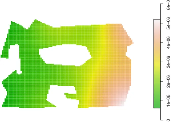
One of the important questions about a point pattern dataset is whether it can be treated as spatially homogeneous. To investigate this, Diggle and others have recommended kernel smoothing. The function ksmooth.ppp performs kernel smoothing of a point pattern, and yields a pixel image object.
0 1e−06 2e−06 3e−06 4e−06 5e−06 6e−06
Figure 11: Kernel smoothed intensity estimate for the point pattern in Figure2, indicating a clear trend from left to right.
spatstatcontains several functions which extend classical techniques (developed for
homoge-neous patterns) to inhomogehomoge-neous point patterns. They includeKinhom (an inhomogeneous version of theK functionBaddeleyet al. (2000)) and the model-fitting function ppm.
7.3. Summary statistics for unmarked point patterns
Exploratory analysis of point patterns is based largely on summary statistics. The spatstat
package will compute estimates of the summary functions
F(r), the empty space function (contact distribution or ‘point-to-event’ distribution) G(r), the nearest neighbour distance distribution function (‘event-to-event’ distribution) J(r), the function J = (1−G)/(1−F)
K(r), the reduced second moment function (”Ripley’sK function”) g(r), the pair correlation functiong(r) = [drdK(r)]/(2πr)
for a point pattern, and their analogues for marked point patterns.
These estimates can be used for exploratory data analysis and in formal inference about a spatial point pattern. They are well described in the literature, e.g. Ripley (1981), Diggle
(2003), Cressie (1991), (Stoyan et al. 1995, Chapter 15), Stoyan and Stoyan (1995). The J-function was introduced in van Lieshout and Baddeley (1996).
The point pattern is assumed to be stationary (homogeneous under translations) in order that the functionsF, G, J, K be well-defined and the corresponding estimators approximately unbiased. (There is an extension of theK function to inhomogeneous patterns; see below). The corresponding spatstat library functions are:
Fest estimate of empty space function F
Gest estimate of nearest neighbour distribution functionG
Jest estimate ofJ-function
Kest estimate of Ripley’s K-function
allstats estimates of all four functions F, G, J, K
pcf estimate of pair correlation function g (Some others are listed below).
In each of these commands, the user has a choice of several alternative estimation methods. These estimators are based on different ‘edge corrections’, or strategies for removing the bias due to ‘edge effects’, which arise because we only observe the point pattern inside a restricted spatial window. Several dozen alternative edge corrections have been published in the literature; seeBaddeley(1998);Stoyan and Stoyan(1995) for surveys. Part of thespatstat
project is to implement all of these proposed estimators so that they may be compared in practice.
The routinesFest, Gest, Jest, Kest, pcfeach return an object of class"fv" (for “func-tion value”). This is a data frame with some extra attributes indicating the recommended way of plotting the function, and other information. It is a convenient way of storing (particularly for use in future plotting) several different estimates of the same function.
A column labelled r in this data frame contains the values of the argument r for which the summary function (Fb(r), etc) has been evaluated. Other columns give the estimates of the summary function itself, using several competing estimators. Along with the different function estimates, the data frame includes the vector of theoretical expected values (theo) that the function would have under the assumption of “complete spatial randomness” (CSR) i.e. under a homogeneous Poisson point process model.
There are methods for print and plot for the class "fv". The plot method is particularly useful. It is a generalisation of plot.formula, and enables the summary functions to be re-plotted in a variety of ways.
There are various recommendations in the literature about how to plot the summary functions to reveal diagnostic information. An aim ofspatstatis to make it easy to plot the summary functions in different ways.
Probably the most common exploratory graphic is a plot of Kb(r) against r. An example of a useful transformed graphic is a plot ofL(r) =
q b
K(r)/πagainstr, as recommended byRipley
(1981), the rationale being that this procedure linearizes the plot and stabilizes the variance.
Diggle (1983, 2003) recommends plotting Kb(r)−πr2 against r, so as to remove the mean.
These plots can be achieved as follows: R> Kc <- Kest(cells)
r K(r) 0 2 4 6 8 10 0 50 100 150 200 250 data Poisson
Figure 12: Output of plot(Kest(X)).
R> plot(Kc, cbind(r, sqrt(iso/pi)) ~ r)
R> plot(Kc, cbind(trans,iso,border) - theo ~ r)
Notice the use ofcbindin the last two plots. The effect is that several functions (the columns in thecbind expression on the left hand side) will be plotted in the same plot, against the variable on the right hand side of the formula.
With respect to the empty space (contact) distribution functionF,Ripley(1981,1988) simply plots Fb(r) against r, whereas Diggle (2003) plots Fb(r) against F0(r) = 1−exp{−λπrˆ 2},
this being the form of F under the assumption of complete spatial randomness. This is in effect a P–P plot. Another useful graphic (suggested by Murray Aitkin) is a plot of sin−1(
q b
F(r)) against sin−1(pF0(r)). The function g(x) = sin−1
√
x is Fisher’s variance-stabilising transformation for the binomial estimator of a proportion, and indeed seems to approximately stabilise the variance in this context.
These alternative plots may be displayed as follows.
R> Fc <- Fest(cells) R> plot(Fc)
R> plot(Fc, cbind(km, trans, border) ~ theo) R> fisher <- function(x) { asin(sqrt(x)) } R> plot(Fc, fisher(cbind(km, trans, border))
~ fisher(theo))
Initially it may be unclear which of the summary functions will provide insight, and it is usu-ally desirable to calculate and plot estimates of all four. The commandplot(allstats(X))
will produce a plot of estimates of the four main summary functionsK,F,Gand J. Distances between points are also computed (without edge correction) by:
nndist nearest neighbour distances
pairdist distances between all pairs of points
exactdt distance from any location to nearest data point
There are also several related alternative functions. For the second order statistics, alterna-tives are:
Kinhom K function for inhomogeneous point patterns
Kest.fft fastK-function using FFT for large datasets
Kmeasure reduced second moment measure
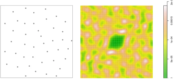
The function Kmeasureyields a pixel image of the estimated Reduced Second Moment Mea-sure K (see (Stoyan and Stoyan 1995, p. 245)). This measure is the Fourier transform of the Bartlett spectrumBartlett(1964,1975). Although first defined in the 1960’s this concept ap-pears not to have been implemented in software until recently. Its usefulness in data analysis is yet to be explored. 0 5e−05 1e−04 0.00015 2e−04
Figure 13: The cells dataset (Left) and a density estimate of its second moment measure (Right).
Figure13 shows the well-knowncells dataset, and a density estimate of its second moment measure, computed byKmeasure. [The algorithm takes the raw Bartlett periodogram, mul-tiplies by the Fourier transform of the bivariate normal density, then takes the inverse FFT to yield the smoothed density.] The large contour in the centre of the Figure is a region of low second moment density close to the origin, caused by the spatial inhibition between points at short distances. The pronounced non-circular shape of this contour suggests that the interpoint interaction is anisotropic, which does not appear to have been noticed before.
8. Summary statistics for multitype point patterns
Analogues of the G, J and K functions have been defined in the literature for “multitype” point patterns, that is, patterns in which each point is classified as belonging to one of a finite number of possible types (e.g. on/off, species, colour). The best known of these is the bivariate (cross)K functionKij(r) derived by counting, for each point of typei, the number
of typej points lying closer thanr units away.
The corresponding nearest-neighbour functionGij(r) is the distribution of the distance from a typical point of typei to the nearest point of typej. Using the symbol •to denote points of any type (i.e. all points regardless of their type) we may define analogous functions Ki•
andGi•. For further explanation seevan Lieshout and Baddeley (1999).
Gcross,Gdot,Gmulti multitype nearest neighbour distributions Gij, Gi•
Kcross,Kdot, Kmulti multitype K-functions Kij, Ki•
Jcross,Jdot,Jmulti multitype J-functions Jij, Ji•
These functions operate in a very similar way toGest, Jest, Kestwith additional arguments specifying the type(s) of points to be studied.
8.1. Function arrays
For multitype patterns we might want to compute a summary function for the points of type i for each of the possible types of the pattern. Alternatively we might want to compute a summary function for each possible pair of types (i, j).
Afunction array is a collection of functionsfi,j(r) indexed by integersiand j. An example is the set of cross K functions Kij(r) for all possible pairs of types i and j in a multitype point pattern (1≤i, j≤m wherem is the number of types). It is best to think of this as a genuine matrix or array.
A function array is represented inspatstat by an object of type "fasp" (function array for spatial patterns). It can be stored, plotted, indexed and subsetted in a natural way. If Zis a function array, then
R> plot(Z)
R> plot(Z[,3:5])
will plot the entire array, and then plot the subarray consisting only of columns 3 to 5. The function alltypes will compute a summary statistic for each possible type, or each possible pair of types, in a multitype point pattern. The value returned by alltypes is a function array object.
For example if Xis a multitype point pattern with 3 possible types, R> Z <- alltypes(X, "K")
yields a 3×3 function array such that (say) Z[1,2] represents the cross-type K function K1,2(r) between types 1 and 2.
The commandplot(Z)will then plot the entire set of crossK functions as a two-dimensional array of plot panels. Arguments toplot.fasp can be used to change the plotting style, the range of the axes, and to select which estimator ofKij is plotted. These options apply to all the plot panels simultaneously.
The commandallstatsyields a 2×2 function array containing theF,G,J andK functions of an (unmarked) point pattern.
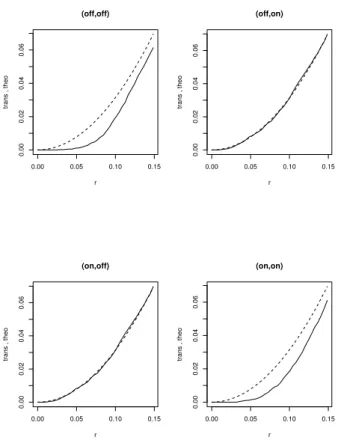
0.00 0.05 0.10 0.15 0.00 0.02 0.04 0.06 r trans , theo (off,off) 0.00 0.05 0.10 0.15 0.00 0.02 0.04 0.06 r trans , theo (off,on) 0.00 0.05 0.10 0.15 0.00 0.02 0.04 0.06 r trans , theo (on,off) 0.00 0.05 0.10 0.15 0.00 0.02 0.04 0.06 r trans , theo (on,on) Array of K functions for amacrine.
Figure 14: The result of plot(alltypes(amacrine, "K")).
8.2. Summary functions for point patterns with continuous marks
Some point pattern datasets are marked, but not multitype. That is, the points may carry marks that do not belong to a finite list of possible types. The marks might be continuous numerical values, complex numbers, etc.
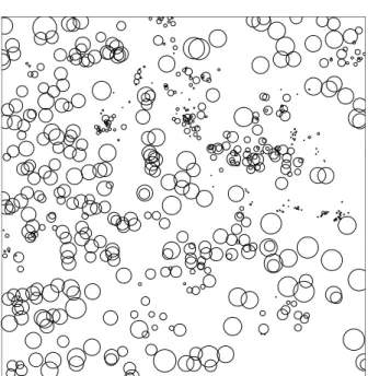
An example is the Longleaf Pines data (shown in Figure 6) where the marks represent tree diameters. Inspatstat, a marked point pattern with numerical marks is plotted using circles of radius proportional to the positive marks, and squares of side length proportional to the negative marks.
There are a few ways to study such patterns inspatstat. The function markcorr computes the mark correlation function of an arbitrary marked point pattern. The functions Kmulti,
Gmulti, Jmulti operate on arbitrary marked point patterns. They require arguments I, J
identifying two subsets of the point pattern. These two subsets will be treated as two discrete types.
Alternatively a marked point pattern can be converted to a multitype point pattern using the functioncut.ppp, for example, classifying the marks into High, Medium and Low. Then one can apply the abovementioned functions for multitype point patterns. This is usually a good exploratory step, along with the use of split.ppp to separate the sub-patterns. Of course one can also ignore the marks (using the functionunmark to remove them) and analyse only
the locations of the points.
9. Model fitting
The most important feature ofspatstatis its ability to fit parametric models of spatial point processes to point pattern data. The scope of possible models is very wide: they may include spatial trend, dependence on covariates, interpoint interactions of any order (i.e. we are not restricted to pairwise interactions), and dependence on marks.
Models are fitted by a functionppmwhich is analogous toglmandlm. The fitted model objects can be printed, plotted, predicted, and even simulated. Methods for computing residuals and plotting model diagnostics will be released in version 1.6.
Models are currently fitted by the method of maximum pseudolikelihood, using a computa-tional device developed byBerman and Turner(1992) which we adapted to pseudolikelihoods
in Baddeley and Turner (2000). Although maximum pseudolikelihood may be statistically
inefficient, it has the virtue that we can implement it in software with great generality. Future versions of the package will implement other fitting methods.
9.1. Formulating models
The point process models fitted byppmare formulated in terms of their conditional intensity
rather than their likelihood. The (Papangelou) conditional intensity is a function λ(u,x) of spatial location u and of the entire point pattern x. See Baddeley and Turner (2000); Cox
and Isham(1980) and the excellent surveys by Ripley(1988,1989).
For example, the homogeneous Poisson process (complete spatial randomness, CSR) has con-ditional intensity
λ(u,x) =β
whereβ is the expected number of points per unit area. The inhomogeneous Poisson process with intensity function β(u) has conditional intensity
λ(u,x) =β(u). (1)
The Strauss process, a simple model of dependence between points, has conditional intensity
λ(u,x) =βγt(u,x) (2)
wheret(u,x) is the number of points of xthat lie within a distancer of the location u. Here r, β >0 andγ ∈[0,1] are parameters.
Our technique fits any model which belongs to the regular exponential family of distributions and which has a conditional intensity. The conditional intensity can then be written in the form
λ(u,x) = exp(θTB(u) +ϕTC(u,x)) (3) where θ, ϕ are the canonical parameters. Both θ and ϕ may be vectors of any dimension, corresponding to the dimensions of the vector-valued statisticsB(u) andC(u,x) respectively. The term B(u) depends only on the spatial location u, so it represents “spatial trend” or spatial covariate effects. The termC(u,x) represents “stochastic interactions” or dependence
between the points of the random point process. For example it is absent if the model is a Poisson process.
The Strauss process (2) with fixed interaction range r conforms to (3) if we set θ = logβ, ϕ= logγ,B(u)≡1 and c(u,x) =t(u,x).
9.2. Fitting a model to data
Overview
The model-fitting function is called ppm and is strongly analogous to lm or glm. In simple usage, it is called in the form
ppm(X, trend, interaction, ...)
whereXis the point pattern dataset, trend is an Slanguage formula describing the spatial trend (the function B(u) in equation 3), and interaction is an object of a special class
"interact"describing the stochastic dependence between points in the pattern (the function
C(u,x) in equation (3)). Other arguments may provide covariates and control the fitting algorithm.
Thus, the function B(u) in (3) is treated as the ‘systematic’ component of the model, and is described by a formula analogous to the formula for the linear predictor in a generalised linear model. In this analogy the link is always the logarithm, so the model formula in appm
call is always a description of thelogarithmof the conditional intensity.
The functionC(u,x) in (3) is regarded as a “distributional” component of the model analogous to the distribution family in a generalised linear model. It is described inspatstatby an object of class"interact"that we create using specialisedspatstatfunctions, similar to those which create thefamily argument toglm.
For example
R> ppm(X, ~1, Strauss(r=0.1), ....)
fits the stationary Strauss process with interaction radiusr= 0.1. The spatial trend formula
~1 is a constant, meaning the process is stationary. The argument Strauss(r=0.1) is an object representing the interpoint interaction structure of the Strauss process with interaction radiusr= 0.1. Similarly
R> ppm(X, ~x + y, Poisson())
fits the non-stationary Poisson process with aloglinear intensity of the form β(x, y) = exp(θ0+θ1x+θ2y)
where θ0, θ1, θ2 are (scalar) parameters to be fitted, and x, y are the cartesian coordinates.
Similarly a log-quadratic intensity in x,
β(x, y) = exp(θ0+θ1x+θ2x2)
R> ppm(X, ~x + I(x^2), Poisson())
Spatial trend
Thetrend argument of ppmdescribes any spatial trend and covariate effects. The default is
~1, which corresponds to a process without spatial trend or covariate effects. The formula~x
corresponds to a spatial trend of the formλ(x, y) = exp(a+bx), while~x + ycorresponds to λ(x, y) = exp(a+bx+cy) where x, yare the Cartesian coordinates. These could be replaced by any Rlanguage formula (with empty left hand side) in terms of the reserved names x, y
andmarks, or in terms of some spatial covariates which you must then supply to ppm. There
is no restriction on the formula since the functionB(u) in (3) is arbitrary.
The trend formula may be an arbitrary expression involving the Cartesian coordinates. For example
R> ppm(X, ~ sqrt(x^2 + y^2), Poisson())
fits an inhomogeneous Poisson process with intensity decaying or increasing exponentially with distance from the origin, while
R> ppm(X, ~ factor(ifelse(x > 2, 0, 1)), Poisson())
fits an inhomogeneous Poisson process with different, constant intensities on each side of the linex= 2.
spatstat provides a function polynom which generates polynomials in 1 or 2 variables. For
example
~ polynom(x, y, 2)
represents a polynomial of order 2 in the Cartesian coordinates x and y. This would give a “log-quadratic” spatial trend.2 Similarly
~ harmonic(x, y, 2)
represents the most generalharmonic polynomial of order 2 in x and y.
Other possibilities include B-splines and smoothing splines, fitted withbsand srespectively. These terms introduce smoothing penalties, and thus provide an implementation of “penalised maximum pseudolikelihood” estimation (cf.Divino, Frigessi, and Green(2000)). For example
R> ppm(X, ~bs(x,2), Poisson())
fits a non-stationary Poisson process whose log conditional intensity is modelled by a B-spline with 2 degrees of freedom.
The special termoffsetcan also be used in the trend formula. It has the same role inppmas it does in other model-fitting functions, namely to add to the linear predictor a term which is not associated with a parameter. For example
2We caution against using the standard function
poly for the same purpose here. For a model formula containingpoly, prediction of the fitted model can be erroneous, for reasons which are well-known toRusers. The functionpolynomprovided inspatstatdoes not exhibit this problem.
~ offset(3 * sin(x))
will fit the model with log trendβ+ 3 sinx whereβ is the only parameter to be estimated. It is slightly more tricky to includeobserved spatial covariates; see Section9.6below.
Interaction terms
The higher order (“interaction”) structure can be specified using one of the following functions. They yield an object (of class"interact") describing the interpoint interaction structure of the model.
Poisson. . . Poisson process
Strauss. . . Strauss process
StraussHard. . . Strauss process with a hard core
Softcore. . . Pairwise soft core interaction
PairPiece. . . Pairwise interaction, step function potential
DiggleGratton . . . Diggle-Gratton potential
LennardJones . . . . Lennard-Jones potential
Geyer. . . Geyer’s saturation process
OrdThresh. . . Ord’s process, threshold on cell area
Note that ppmestimates only the “canonical” parameters of a point process model. These are parameters θ such that the loglikelihood is linear in θ, as in equation (3), possibly after a re-parametrisation.
Other so-called “irregular” parameters (such as the interaction radiusrof the Strauss process) cannot be estimated directly by this technique, and their values must be specified a priori, as arguments to the interaction function. Profile pseudolikelihood Baddeley and Turner (2000) can be used to fit such parameters.
For more advanced use, the following functions will accept “user-defined potentials” in the form of an arbitrary S language function. They effectively allow arbitrary point process models of these three classes.
Pairwise. . . . Pairwise interaction, user-supplied potential
Ord. . . Ord model, user-supplied potential
Saturated. . . Saturated pairwise model, user-supplied potential
9.3. Fitted models
The value returned by ppmis a “fitted point process model” of class "ppm". It can be stored, inspected, plotted and predicted.
R> fit <- ppm(X, ~1, Strauss(r=0.1), ...) R> fit
R> plot(fit)
R> pf <- predict(fit) R> coef(fit)
Methods are provided for the following generic operations applied to"ppm"objects:
print Print basic information
summary Print extensive summary information
coef Extract fitted model coefficients
plot Plot fitted intensity
fitted Compute fitted conditional intensity or trend at data points
predict Compute predictions (spatial trend, conditional intensity)
update Update the fit
Printing the fitted object fit will produce text output describing the fitted model in its traditional form. For example, the traditional parametersβ, γ of the Strauss process (2) are not in canonical form (3). The print method back-transforms the fitted canonical parameter θto the traditional parameters β and γ.
Plotting the fitted model object will display the spatial trend and the conditional intensity, as perspective plots, contour plots and image plots.
The predict method computes either the spatial trend or the conditional intensity. The
default behaviour is to produce a pixel image of both trend and conditional intensity, where these are appropriate. The conditional intensity λ(u,x) can be evaluated at any desired locationsu, butx is taken to be the observed data pattern to which the model was fitted. Examples of calls topredict.ppm are the following:
R> data(cells)
R> m <- ppm(cells,~polynom(x,y,2),Strauss(0.05), rbord=0.05)
R> trend <- predict(m,type="trend",ngrid=100) R> cif <- predict(m,type="cif",ngrid=100)
The resulting objects trend and cif are pixel images. One could then plot the resulting surfaces with calls like
R> persp(trend,theta=-30,phi=40,d=4, ticktype="detailed",zlab="z") R> persp(cif,theta=-30,phi=40,d=4,
ticktype="detailed",zlab="z")
We note again that the result ofpredictmay be incorrect if the point process model’s trend component is expressed in terms of one of the functionspoly,bs,lo, orns.
The plot method (plot.ppm) will take a fitted point process model and plot the trend and/or the conditional intensity. By default this surface is calculated at a 40×40 grid of points on the (enclosing rectangle of) the observation window. The plots may be produced as perspective plots, images, or contour plots. A simple example is
R> plot(fit,cif=FALSE,how="persp")
x 2 4 6 8 y 2 4 6 8 z 1 2 3 4 5
Figure 15: Fitted log-cubic trend for the full Numata pines data set obtained using
predict.ppm.
9.4. In defence of maximum pseudolikelihood
Disadvantages of maximum pseudolikelihood (MPL) include its small-sample bias and in-efficiency Besag (1977); Jensen and Møller (1991); Jensen and K¨unsch (1994) relative to maximum likelihood estimators (MLE).
However, as far as we are aware, there is currently no software implementation of any MLE technique for fitting point process models at the level of generality and flexibility that is achieved in spatstat. Numerical approximation methods Ogata and Tanemura (1986) and Markov Chain Monte Carlo methods Geyer and Møller(1994);Geyer (1999) are highly spe-cific to the chosen model, and require careful tuning to ensure good performance. Markov Chain Monte Carlo is computationally intensive, especially for inhomogeneous spatial pat-terns, because of increased parameter dimensionality. Recent theoretical improvementsGeyer
and Møller(1994);Geyer(1999) have not yet led to better software implementations.
Thus, maximum pseudolikelihood has several advantages. It is extremely fast in execution, compared to the MLE. Our new implementation of the MPLE also enables new models to be specified very easily, and accommodates a wide range of models.
In real data analysis, the model should be regarded as tentative, and a fitted model should be criticised or validated, and possibly modified and re-fittedChatfield(1988);Cox and Snell
(1981);Davison and Snell (1991); Tukey (1977); Venables and Ripley (1997). The accuracy
of the fitting procedure is not the only consideration. Hence, there is an important place for quick-and-dirty fitting methods especially in the analysis of real datasets.
When ppm is used, fitting a model encompassing both spatial inhomogeneity and interpoint interaction becomes routine. For example we can fit the model chosen for the Numata data
inOgata and Tanemura(1986) as follows:
In any case, more accurate estimation algorithms usually require a good starting value of the parameter estimate, and it is universally the MPL estimate which is used. Thus, an implementation of MPL is a prerequisite to implementing other techniques.
9.5. Fitting models to multitype point patterns
The functionppmwill also fit models to multitype point patterns. A multitype point pattern is a point pattern in which the points are each classified into one of a finite number of possible types (e.g. species, colours, on/off states). Inspatstata multitype point pattern is represented
by a"ppp"object Xwhose marks are a factor. Figure7 shows an example.
Currently,ppmwill not fit models to a marked point pattern if the marks are not a factor.
Trend component
The first-order component (“trend”) of a multitype point process model may depend on the marks. For example, a stationary multitype Poisson point process could have different (con-stant) intensities for each possible mark. A general nonstationary process could have a dif-ferent spatial trend surface for each possible mark.
In order to represent the dependence of the trend on the marks, the trend formula passed to
ppm may involve the reserved name marks.
The trend formula ~1 states that the trend is constant and does not depend on the marks. The formula ~marks indicates that there is a separate, constant intensity for each possible mark. The correct way to fit the multitype Poisson process is
R> ppm(X, ~ marks, Poisson())
The result of fitting this model to the data in Figure7yields the following output.
Stationary multitype Poisson process Possible marks:
off on Intensity:
Trend formula: ~marks Fitted intensities:
beta_off beta_on
88.68302 94.92830
This indicates that the fitted model is a multitype Poisson process with intensities 88.7 and 94.9 for the points of type “off” and “on” respectively.
Getting more elaborate, the trend formula might involve both the marks and the spatial locations or spatial covariates. For example the trend formula ~marks + polynom(x,y,2)
signifies that the first order trend is a log-quadratic function of the cartesian coordinates, multiplied by a constant factor depending on the mark.
The formulae
~ marks * polynom(x,2)
both specify that, for each mark, the first order trend is a different log-quadratic function of the cartesian coordinates. The second form looks “wrong” since it includes a “marks by
polynom” interaction without havingpolynomin the model, but sincepolynomis a covariate
rather than a factor this is is allowed, and makes perfectly good sense. As a result the two foregoing models are in fact mathematically equivalent. However, the fitted model objects will give slightly different output.
For example, the first model~marks * polynom(x,2)fitted to the data in Figure7gives the following output (assuming options("contrasts") is set to its default, namely the ‘treat-ment’ contrasts):
Nonstationary multitype Poisson process Trend formula: ~marks * polynom(x, 2) Fitted coefficients for trend formula:
(Intercept) markson 4.3127945 0.2681231 polynom(x, 2)[x] polynom(x, 2)[x^2] 0.4651860 -0.2363352 markson:polynom(x, 2)[x] markson:polynom(x, 2)[x^2] -0.6781045 0.4023491
This form of the model gives two quadratic functions: a “baseline” quadratic P0(x, y) = 4.3127945 + 0.4651860x−0.2363352x2
and a quadratic associated with the mark level “on”,
Pon(x, y) = 0.2681231−0.6781045x+ 0.4023491x2.
The baseline quadratic is the logarithm of the fitted trend for the points of typeoff, sinceoff
is the first level of the factor marks. For points of type on, since we are using the treatment contrasts, the log trend is
P0(x, y) +Pon(x, y) = 4.580918−0.2129185x+ 0.1660139x2.
On the other hand, when the second model ~marks + marks:polynom(x,2) is fitted to the same dataset, the output is
Nonstationary multitype Poisson process Trend formula: ~marks + marks:polynom(x, 2) Fitted coefficients for trend formula:
(Intercept) markson 4.3127945 0.2681231 marksoff:polynom(x, 2)[x] markson:polynom(x, 2)[x] 0.4651860 -0.2129185 marksoff:polynom(x, 2)[x^2] markson:polynom(x, 2)[x^2] -0.2363352 0.1660138
This says explicitly that the log trend for points of typeoff is
Qoff(x, y) = 4.3127945 + 0.4651860x−0.2363352x2
while for points of typeonit is
Qon(x, y) = 4.580918−0.2129185x+ 0.1660139x2.
Hence the two fitted models are mathematically identical.
Interaction component
For the interaction component of a multitype point process model, any of the interaction structures listed above for unmarked point processes may be used. These interactions do not depend on the marks, only on the locations of the points. We have additionally defined two interactions which do depend on the marks:
MultiStrauss multitype Strauss process
MultiStraussHard multitype Strauss/hard core
For the multitype Strauss process, a matrix of “interaction radii” must be specified. If there arem distinct levels of the marks, we require a matrix r in whichr[i,j] is the interaction radius rij between types i and j. For the multitype Strauss/hard core model, a matrix of “hardcore radii” must be supplied as well. These matrices will be of dimension m×m and
must be symmetric.
9.6. Models with covariates
We can also fit point process models in which the point pattern is dependent on spatial covariates (e.g. altitude, soil pH, or distance to another spatial pattern). Any covariate data may be used, under the following conditions:
• the covariate must be a quantity Z(u) observable (at least in principle) at each location u in the window. There may be several such covariates, and they may be continuous valued or factors.
• the values Z(xi) of Z at each point of the data point pattern must be available.
• the values Z(u) at some other points uin the window must be available. 3
Thus, it is not enough simply to observe the covariate values at the points of the data point pattern. For example, a dataset consisting of locations of trees in a forest and measurements of the soil acidity at these locations only, is not sufficient data to fit a model in which tree density depends on pH.
Covariate data are passed to the functionppmthrough the argument covariates. It may be either a data frame or a list of pixel images.
3The accuracy of the algorithm depends on the number of these points and on their spatial arrangement.
For a good approximation to the pseudolikelihood, the density of these points should be high throughout the window.
(a) If covariatesis a list of pixel images, then each image is assumed to contain the values of a spatial covariate. The names of the entries in the list should match the names of covariates used in the trend formula. For example:
R> ppm(X, ~ log(altitude) + pH,
covariates=list(pH=phimage,altitude=image3))
(b) If covariatesis a data frame, then theith row of the data frame is expected to contain the covariate values for the ith ‘quadrature point’ (see below). The column names of the data frame should match the names of the covariates used in the trend formula. For example:
R> ppm(X, ~ log(altitude) + pH, covariates=cov.df)
where cov.df is a data frame with columns calledpH andaltitude.
Covariates in a list of images
The format (a), in which covariates is a list of images, would typically be used when the covariate values are already given on a fine grid (e.g. satellite image data, geological survey data) or are easy to obtain in this form.
Suppose X is a point pattern representing the locations of alpine ash trees, and A is a pixel image containing values of the terrain elevation in metres above sea level. Then
R> ppm(X, ~bs(alt, 2), covariates=list(alt=A))
fits the inhomogeneous Poisson process model where the density of trees depends on elevation through a B-spline with 2 degrees of freedom.
It is also convenient to supply covariates in the pixel image format when the covariate value can easily be computed at any location from existing data. For example, Figure9 shows a pixel image of covariate values derived from thecopper dataset. The covariate valueZ(u) at pixelu is the distance from uto the nearest line segment in the copper dataset.
Covariates in a data frame
Typically you would use the data frame format (b) if the values of the spatial covariates can only be observed at certain fixed locations. You need to forceppm to use these locations to fit the model.
This requires a little more information about the software. Our functionppmis an implementa-tion of the algorithm ofBaddeley and Turner(2000) which is based on a quadrature technique originated byBerman and Turner(1992). Very briefly, a ‘quadrature scheme’ inspatstat com-prises both‘data points’ (the points of the observed point pattern) and‘dummy points’ (some other locations in the window). It is usually created using the functionquadscheme.
You will need to create a quadrature scheme based on the spatial locations where the covariate Z has been observed. Then the values of the covariate at these locations are passed to ppm
through the data framecovariates.
For example, suppose that X is the observed point pattern and we are trying to model the effect of soil acidity (pH). Suppose we have measured the values of soil pH at the points xi
of the point pattern, and stored them in a vectorXpH. Suppose we have measured soil pH at some other locationsu in the window, and stored the results in a data frameUwith columns
x, y, pH. Then do as follows:
R> Q <- quadscheme(data=X, dummy=list(x=U$x, y=U$y)) R> df <- data.frame(pH=c(XpH, U$pH))
Then the rows of the data frame df correspond to the quadrature points in the quadrature schemeQ. To fit just the effect of pH, type
R> ppm(Q, ~ pH, Poisson(), covariates=df)
where the term pH in the formula ~ pH agrees with the column label pH in the argument
covariates = df. This will fit an inhomogeneous Poisson process with intensity that is a
loglinear function of soil pH. You can also try (say) R> ppm(Q, ~ pH, Strauss(r=1), covariates=df)
R> ppm(Q, ~ factor(pH > 7), Poisson(), covariates=df) R> ppm(Q, ~ polynom(x, 2) * factor(pH > 7), covariates=df)
9.7. Offset terms
As we mentioned in section9.2, the special termoffsetcan also be used in the trend formula. It has the same role in ppmas it does in other model-fitting functions, namely to add to the linear predictor a term which is not associated with a parameter.
This is specially useful in case-control studies. For example, suppose we have a spatial epi-demiological dataset containing a point pattern X of the locations of cases of a rare disease, and another point patternYof ‘controls’ which are a sample from the susceptible population. We want to modelXas a point process with intensity proportional to the local densityρof the susceptible population. We estimateρ by taking a kernel-smoothed estimate of the intensity of Y. Thus
R> rho.hat <- ksmooth.ppp(Y, sigma=1.2)
R> ppm(X, ~offset(log(rho)), covariates=list(rho=rho.hat))
The first line computes the values of the kernel-smoothed intensity estimate at a fine grid of pixels, and stores them in the pixel image object rho.hat. The second line fits the Poisson process model with log intensity
logλ(u) =θ+ logρ(u)
where θis an unknown parameter; that is, it fits the Poisson model with intensity λ(u) =β ρ(u)
whereβ=eθ is the only parameter to be estimated. Note that covariatesmust be a list of images, even though there is only one covariate. The variable namerhoin the model formula must match the namerhoin the list.
10. Simulation
Stochastic simulation of point process models is another area where the richness of the theo-retical literature contrasts with the scarcity of stable public domain software.
The spatstat package now has substantial functionality for simulating point processes. In
particular it has the powerful ability to simulate a pattern directly from a fitted model. The following functions generate random point patterns from various stochastic models. We follow theRnaming convention that a random generator is calledrdistwheredistis the name of the probability distribution. These functions return a point pattern (as an object of class
"ppp").
runifpoint n independent random points
uniform in window
rpoint n independent random points
with given density
rmpoint n independent multitype random
points with given density
rpoispp (in)homogeneous Poisson process
rmpoispp multitype (in)homogeneous Poisson
rMaternI Mat´ern Model I inhibition process Mat´ern(1986)
rMaternII Mat´ern Model II inhibition processMat´ern(1986)
rSSI Simple Sequential Inhibition
rNeymanScott general Neyman-Scott process
rMatClust Mat´ern Cluster processMat´ern(1986)
rThomas Thomas process
rmh run Metropolis-Hastings algorithm
SeeDiggle(2003);Møller and Waagepetersen (2003);Stoyan and Stoyan (1995) for
informa-tion about these models. For example R> plot(rMaternI(200,0.05))
will plot one realisation of the Mat´ern Model I inhibition process with parameters β = 200 andr = 0.05. See Figure16.
The function rmh enables simulation from a broad range of point process models. It will also simulate any of the fitted models obtained from ppm, with a few exceptions (currently
LennardJonesand OrdThresh.)
10.1. Poisson processes
Simulation of Poisson processes is effected by the function rpoispp. This will simulate both homogeneous and inhomogeneous Poisson processes, in arbitrary windows — polygons, poly-gons with “holes”, and masks, as well as in rectangles. The intensity function of the Poisson process may be specified by a constant, by an Rlanguage function of the coordinatesx and y, or by a pixel image. For example, the commands
R> lambda <- function(x, y) { 100 * exp( 3 * x) } R> X <- rpoispp(lambda, win=square(1))
rMaternI(100, 0.05) • • • • • • • • • • • • • • • • • • • • • • • • • • • • • • • • • • • • • • • • • • • •
Figure 16: Realisation of Mat´ern Model I process.
generate a realisation of the Poisson process with intensity function λ(x, y) = 100e3x in the unit square.
There is also a functionrpoint which generates afixed number of points in a given window, again of arbitrary shape, with an arbitrary probability density. The probability density may again be specified by a constant, a function(x,y), or a pixel image, and does not need to be normalised.
Examples:
R> data(letterR)
R> X1 <- rpoispp(100,win=letterR) R> X2 <- rpoint(100,win=letterR)
The point patternX1 will have about 370 points in it since the area of letterR is about 3.7 units. (To find this out one can use area.owin(letterR).) The point pattern X2 will have exactly 100 points.
10.2. Doubly-stochastic processes
In a “doubly stochastic” or two-stage model, we first generate points at random according to a simple mechanism (usually the Poisson process) and then modify the pattern by randomly deleting or adding or moving some of the points.
The doubly stochastic mechanisms in spatstat for generating point patterns are the Mat´ern I and II models, the Mat´ern cluster process, the Thomas process, and the general Neyman-Scott process with bounded cluster radius. The corresponding function names arerMaternI,
rMaternII,rMatClust,rThomasand rNeymanScott, respectively. The first two mechanisms
are inhibitory — in each case a Poisson process is generated and then thinned. The other three mechanisms generate cluster processes, where the centres of the clusters form a Poisson process. The third and fourth mechanisms are special cases of the fifth.