Divide-and-conquer algorithms
Thedivide-and-conquerstrategy solves a problem by:1. Breaking it intosubproblemsthat are themselves smaller instances of the same type of problem
2. Recursively solving these subproblems 3. Appropriately combining their answers
The real work is done piecemeal, in three different places: in the partitioning of problems into subproblems; at the very tail end of the recursion, when the subproblems are so small that they are solved outright; and in the gluing together of partial answers. These are held together and coordinated by the algorithm’s core recursive structure.
As an introductory example, we’ll see how this technique yields a new algorithm for multi-plying numbers, one that is much more efficient than the method we all learned in elementary school!
2.1 Multiplication
The mathematician Carl Friedrich Gauss (1777–1855) once noticed that although the product of two complex numbers
(a+bi)(c+di) = ac−bd+ (bc+ad)i
seems to involvefourreal-number multiplications, it can in fact be done with justthree: ac, bd, and(a+b)(c+d), since
bc+ad = (a+b)(c+d)−ac−bd.
In our big-Oway of thinking, reducing the number of multiplications from four to three seems wasted ingenuity. But this modest improvement becomes very significantwhen applied recur-sively.
Let’s move away from complex numbers and see how this helps with regular multiplica-tion. Supposexandyare twon-bit integers, and assume for convenience thatnis a power of 2(the more general case is hardly any different). As a first step toward multiplyingxandy, split each of them into their left and right halves, which aren/2bits long:
x= xL xR = 2n/2xL+xR
y= yL yR = 2n/2yL+yR.
For instance, ifx = 101101102 (the subscript2 means “binary”) then xL = 10112, xR = 01102,
andx= 10112×24+ 01102. The product ofxandycan then be rewritten as
xy = (2n/2xL+xR)(2n/2yL+yR) = 2nxLyL + 2n/2(xLyR+xRyL) +xRyR.
We will computexy via the expression on the right. The additions take linear time, as do the multiplications by powers of 2 (which are merely left-shifts). The significant operations are the fourn/2-bit multiplications,xLyL, xLyR, xRyL, xRyR; these we can handle by four recursive
calls. Thus our method for multiplying n-bit numbers starts by making recursive calls to multiply these four pairs of n/2-bit numbers (four subproblems of half the size), and then evaluates the preceding expression in O(n) time. WritingT(n) for the overall running time onn-bit inputs, we get therecurrence relation
T(n) = 4T(n/2) +O(n).
We will soon see general strategies for solving such equations. In the meantime, this particu-lar one works out toO(n2), the same running time as the traditional grade-school
multiplica-tion technique. So we have a radically new algorithm, but we haven’t yet made any progress in efficiency. How can our method be sped up?
This is where Gauss’s trick comes to mind. Although the expression for xy seems to de-mand fourn/2-bit multiplications, as before just three will do:xLyL, xRyR, and(xL+xR)(yL+yR),
sincexLyR+xRyL= (xL+xR)(yL+yR)−xLyL−xRyR. The resulting algorithm, shown in Figure 2.1,
has an improved running time of1
T(n) = 3T(n/2) +O(n).
The point is that now the constant factor improvement, from 4 to 3, occursat every level of the recursion, and this compounding effect leads to a dramatically lower time bound ofO(n1.59).
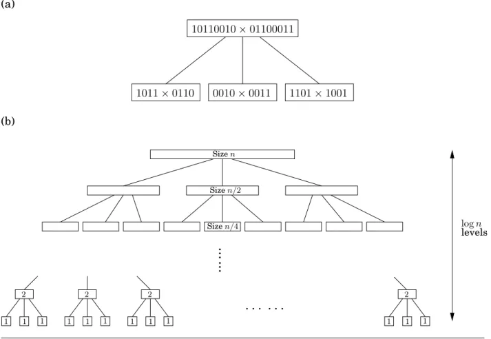
This running time can be derived by looking at the algorithm’s pattern of recursive calls, which form a tree structure, as in Figure 2.2. Let’s try to understand the shape of this tree. At each successive level of recursion the subproblems get halved in size. At the(log2n)th level,
1Actually, the recurrence should read
T(n) ≤ 3T(n/2 + 1) +O(n)
since the numbers(xL+xR)and(yL+yR)could ben/2 + 1bits long. The one we’re using is simpler to deal with and can be seen to imply exactly the same big-Orunning time.
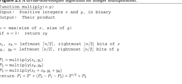
Figure 2.1A divide-and-conquer algorithm for integer multiplication.
function multiply(x, y)
Input: Positive integers x and y, in binary Output: Their product
n= max(size of x, size of y) if n= 1: return xy
xL, xR= leftmost dn/2e, rightmost bn/2c bits of x
yL, yR= leftmost dn/2e, rightmost bn/2c bits of y
P1 =multiply(xL, yL)
P2 =multiply(xR, yR)
P3 =multiply(xL+xR, yL+yR)
return P1×2n+ (P3−P1−P2)×2n/2+P2
the subproblems get down to size 1, and so the recursion ends. Therefore, the height of the tree is log2n. The branching factor is 3—each problem recursively produces three smaller ones—with the result that at depthk in the tree there are3k subproblems, each of sizen/2k.
For each subproblem, a linear amount of work is done in identifying further subproblems and combining their answers. Therefore the total time spent at depthk in the tree is
3k×On 2k = 3 2 k ×O(n).
At the very top level, when k = 0, this works out to O(n). At the bottom, when k = log2n, it is O(3log2n), which can be rewritten as O(nlog23) (do you see why?). Between these two
endpoints, the work done increasesgeometricallyfromO(n)toO(nlog23), by a factor of3/2per
level. The sum of any increasing geometric series is, within a constant factor, simply the last term of the series: such is the rapidity of the increase (Exercise 0.2). Therefore the overall running time isO(nlog23), which is aboutO(n1.59).
In the absence of Gauss’s trick, the recursion tree would have the same height, but the branching factor would be 4. There would be 4log2n = n2 leaves, and therefore the running
time would be at least this much. In divide-and-conquer algorithms, the number of subprob-lems translates into the branching factor of the recursion tree; small changes in this coefficient can have a big impact on running time.
A practical note: it generally does not make sense to recurse all the way down to1bit. For most processors, 16- or 32-bit multiplication is a single operation, so by the time the numbers get into this range they should be handed over to the built-in procedure.
Finally, the eternal question: Can we do better? It turns out that even faster algorithms for multiplying numbers exist, based on another important divide-and-conquer algorithm: the fast Fourier transform, to be explained in Section 2.6.
Figure 2.2Divide-and-conquer integer multiplication. (a) Each problem is divided into three subproblems. (b) The levels of recursion.
(a) 10110010×01100011 1011×0110 0010×0011 1101×1001 (b) 2 1 1 1 2 1 1 1 2 1 1 1 2 1 1 1 Sizen Sizen/2
· · · ·
...
...
logn levels Sizen/42.2 Recurrence relations
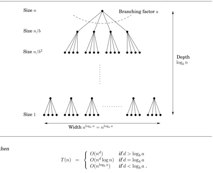
Divide-and-conquer algorithms often follow a generic pattern: they tackle a problem of size nby recursively solving, say,asubproblems of sizen/band then combining these answers in O(nd)time, for somea, b, d >0(in the multiplication algorithm,a= 3,b= 2, andd= 1). Their running time can therefore be captured by the equationT(n) = aT(dn/be) +O(nd). We next derive a closed-form solution to this general recurrence so that we no longer have to solve it explicitly in each new instance.
Master theorem2 If T(n) = aT(dn/be) +O(nd) for some constantsa > 0, b > 1, andd ≥ 0,
Figure 2.3Each problem of sizenis divided intoasubproblems of sizen/b. Size1 Sizen/b2 Sizen/b Sizen Depth logbn
Widthalogbn=nlogba
Branching factora then T(n) = O(nd) ifd >log ba O(ndlogn) ifd= logba O(nlogba) ifd <log
ba.
This single theorem tells us the running times of most of the divide-and-conquer procedures we are likely to use.
Proof. To prove the claim, let’s start by assuming for the sake of convenience that n is a power of b. This will not influence the final bound in any important way—after all, n is at most a multiplicative factor of baway from some power ofb(Exercise 2.2)—and it will allow us to ignore the rounding effect indn/be.
Next, notice that the size of the subproblems decreases by a factor of b with each level of recursion, and therefore reaches the base case after logbn levels. This is the height of the recursion tree. Its branching factor is a, so the kth level of the tree is made up of ak subproblems, each of sizen/bk (Figure 2.3). The total work done at this level is
ak×On bk d = O(nd)×a bd k .
ratioa/bd. Finding the sum of such a series in big-Onotation is easy (Exercise 0.2), and comes down to three cases.
1. The ratio is less than1.
Then the series is decreasing, and its sum is just given by its first term,O(nd). 2. The ratio is greater than1.
The series is increasing and its sum is given by its last term,O(nlogba):
nda bd logbn = nd alogbn (blogbn)d
= alogbn = a(logan)(logba) = nlogba.
3. The ratio is exactly1.
In this case allO(logn)terms of the series are equal toO(nd).
These cases translate directly into the three contingencies in the theorem statement.
Binary search
The ultimate divide-and-conquer algorithm is, of course,binary search: to find a keyk in a large file containing keysz[0,1, . . . , n−1]in sorted order, we first comparekwithz[n/2], and depending on the result we recurse either on the first half of the file,z[0, . . . , n/2−1], or on the second half,z[n/2, . . . , n−1]. The recurrence now isT(n) =T(dn/2e) +O(1), which is the casea = 1, b = 2, d = 0. Plugging into our master theorem we get the familiar solution: a running time of justO(logn).
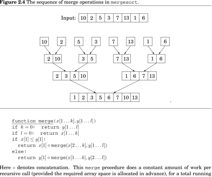
2.3 Mergesort
The problem of sorting a list of numbers lends itself immediately to a divide-and-conquer strategy: split the list into two halves, recursively sort each half, and then merge the two sorted sublists.
function mergesort(a[1. . . n])
Input: An array of numbers a[1. . . n]
Output: A sorted version of this array
if n >1:
return merge(mergesort(a[1. . .bn/2c]), mergesort(a[bn/2c+ 1. . . n])) else:
return a
The correctness of this algorithm is self-evident, as long as a correct merge subroutine is
specified. If we are given two sorted arraysx[1. . . k]andy[1. . . l], how do we efficiently merge them into a single sorted arrayz[1. . . k+l]? Well, the very first element ofz is eitherx[1]or y[1], whichever is smaller. The rest ofz[·] can then be constructed recursively.
Figure 2.4The sequence of merge operations inmergesort. 2 3 5 10 1 6 7 13 10 2 3 5 7 13 1 6 2 5 3 7 13 1 6 10 Input: 10 2 5 3 7 13 1 6 1 2 3 5 6 7 10 13 .
function merge(x[1. . . k], y[1. . . l]) if k = 0: return y[1. . . l]
if l= 0: return x[1. . . k]
if x[1]≤y[1]:
return x[1]◦merge(x[2. . . k], y[1. . . l])
else:
return y[1]◦merge(x[1. . . k], y[2. . . l])
Here ◦ denotes concatenation. This merge procedure does a constant amount of work per
recursive call (provided the required array space is allocated in advance), for a total running time ofO(k+l). Thusmerge’s are linear, and the overall time taken bymergesortis
T(n) = 2T(n/2) +O(n), orO(nlogn).
Looking back at themergesortalgorithm, we see that all the real work is done in
merg-ing, which doesn’t start until the recursion gets down to singleton arrays. The singletons are merged in pairs, to yield arrays with two elements. Then pairs of these 2-tuples are merged, producing 4-tuples, and so on. Figure 2.4 shows an example.
This viewpoint also suggests how mergesortmight be made iterative. At any given
mo-ment, there is a set of “active” arrays—initially, the singletons—which are merged in pairs to give the next batch of active arrays. These arrays can be organized in a queue, and processed by repeatedly removing two arrays from the front of the queue, merging them, and putting the result at the end of the queue.
In the following pseudocode, the primitive operation injectadds an element to the end
of the queue whileejectremoves and returns the element at the front of the queue. function iterative-mergesort(a[1. . . n])
Input: elements a1, a2, . . . , an to be sorted
Q= [ ] (empty queue) for i= 1 to n:
inject(Q,[ai])
while |Q|>1:
inject(Q,merge(eject(Q),eject(Q)))
Annlognlower bound for sorting
Sorting algorithms can be depicted as trees. The one in the following figure sorts an array of three elements,a1, a2, a3. It starts by comparinga1 to a2 and, if the first is larger, compares
it witha3; otherwise it comparesa2 anda3. And so on. Eventually we end up at a leaf, and
this leaf is labeled with the true order of the three elements as a permutation of1,2,3. For example, ifa2 < a1 < a3, we get the leaf labeled “2 1 3.”
3 2 1 Yes a2< a3? a1< a2? a1 < a3? a2< a3? a1 < a3? 2 3 1 2 1 3 3 1 2 1 3 2 1 2 3 No
Thedepthof the tree—the number of comparisons on the longest path from root to leaf, in this case3—is exactly the worst-case time complexity of the algorithm.
This way of looking at sorting algorithms is useful because it allows one to argue that mergesort is optimal, in the sense that Ω(nlogn) comparisons are necessary for sorting n elements.
Here is the argument: Consider any such tree that sorts an array ofnelements. Each of its leaves is labeled by a permutation of{1,2, . . . , n}. In fact,everypermutation must appear as the label of a leaf. The reason is simple: if a particular permutation is missing, what happens if we feed the algorithm an input ordered according to this same permutation? And since there aren!permutations ofnelements, it follows that the tree has at leastn!leaves.
We are almost done: This is a binary tree, and we argued that it has at leastn! leaves. Recall now that a binary tree of depth dhas at most 2d leaves (proof: an easy induction on d). So, the depth of our tree—and the complexity of our algorithm—must be at leastlog(n!).
And it is well known thatlog(n!)≥c·nlognfor somec >0. There are many ways to see this. The easiest is to notice that n! ≥(n/2)(n/2) because n! = 1·2· · · · ·ncontains at least n/2factors larger thann/2; and to then take logs of both sides. Another is to recall Stirling’s formula n!≈ s π 2n+1 3 ·nn·e−n.
Either way, we have established that any comparison tree that sortsnelements must make, in the worst case,Ω(nlogn)comparisons, and hence mergesort is optimal!
Well, there is some fine print: this neat argument applies only to algorithms that use comparisons. Is it conceivable that there are alternative sorting strategies, perhaps using sophisticated numerical manipulations, that work in linear time? The answer is yes, under certain exceptional circumstances: the canonical such example is when the elements to be sorted are integers that lie in a small range (Exercise 2.20).
2.4 Medians
The medianof a list of numbers is its 50th percentile: half the numbers are bigger than it, and half are smaller. For instance, the median of[45,1,10,30,25]is25, since this is the middle element when the numbers are arranged in order. If the list has even length, there are two choices for what the middle element could be, in which case we pick the smaller of the two, say.
The purpose of the median is to summarize a set of numbers by a single, typical value. Themean, or average, is also very commonly used for this, but the median is in a sense more typical of the data: it is always one of the data values, unlike the mean, and it is less sensitive to outliers. For instance, the median of a list of a hundred 1’s is (rightly)1, as is the mean. However, if just one of these numbers gets accidentally corrupted to10,000, the mean shoots up above100, while the median is unaffected.
Computing the median of nnumbers is easy: just sort them. The drawback is that this takesO(nlogn) time, whereas we would ideally like something linear. We have reason to be hopeful, because sorting is doing far more work than we really need—we just want the middle element and don’t care about the relative ordering of the rest of them.
When looking for a recursive solution, it is paradoxically often easier to work with amore generalversion of the problem—for the simple reason that this gives a more powerful step to recurse upon. In our case, the generalization we will consider isselection.
SELECTION
Input: A list of numbersS; an integerk Output: Thekth smallest element ofS
For instance, ifk = 1, the minimum ofS is sought, whereas ifk =b|S|/2c, it is the median. A randomized divide-and-conquer algorithm for selection
Here’s a divide-and-conquer approach to selection. For any numberv, imagine splitting listS into three categories: elements smaller thanv, those equal to v (there might be duplicates), and those greater thanv. Call theseSL,Sv, andSRrespectively. For instance, if the array
S : 2 36 5 21 8 13 11 20 5 4 1
is split onv= 5, the three subarrays generated are
SL: 2 4 1 Sv : 5 5 SR: 36 21 8 13 11 20
The search can instantly be narrowed down to one of these sublists. If we want, say, the eighth-smallest element of S, we know it must be the third-smallest element of SR since |SL| +|Sv| = 5. That is, selection(S,8) = selection(SR,3). More generally, by checking k against the sizes of the subarrays, we can quickly determine which of them holds the desired element: selection(S, k) = selection(SL, k) ifk ≤ |SL| v if|SL|< k≤ |SL|+|Sv| selection(SR, k− |SL| − |Sv|) ifk >|SL|+|Sv|.
The three sublistsSL, Sv, andSRcan be computed fromS in linear time; in fact, this compu-tation can even be donein place, that is, without allocating new memory (Exercise 2.15). We then recurse on the appropriate sublist. The effect of the split is thus to shrink the number of elements from|S|to at mostmax{|SL|,|SR|}.
Our divide-and-conquer algorithm for selection is now fully specified, except for the crucial detail of how to choosev. It should be picked quickly, and it should shrink the array substan-tially, the ideal situation being|SL|,|SR| ≈ 12|S|. If we could always guarantee this situation, we would get a running time of
T(n) =T(n/2) +O(n),
which is linear as desired. But this requires pickingvto be the median, which is our ultimate goal! Instead, we follow a much simpler alternative: we pickvrandomly fromS.
Efficiency analysis
Naturally, the running time of our algorithm depends on the random choices ofv. It is possible that due to persistent bad luck we keep pickingvto be the largest element of the array (or the smallest element), and thereby shrink the array by only one element each time. In the earlier example, we might first pickv = 36, thenv = 21, and so on. This worst-case scenario would force our selection algorithm to perform
n+ (n−1) + (n−2) +· · ·+n
2 = Θ(n
2)
operations (when computing the median), but it is extremely unlikely to occur. Equally un-likely is the best possible case we discussed before, in which each randomly chosen v just happens to split the array perfectly in half, resulting in a running time of O(n). Where, in this spectrum fromO(n)toΘ(n2), does theaveragerunning time lie? Fortunately, it lies very close to the best-case time.
To distinguish between lucky and unlucky choices ofv, we will callv goodif it lies within the 25th to 75th percentile of the array that it is chosen from. We like these choices of v because they ensure that the sublistsSL andSRhave size at most three-fourths that ofS(do you see why?), so that the array shrinks substantially. Fortunately, good v’s are abundant: half the elements of any list must fall between the25th to75th percentile!
Given that a randomly chosenvhas a50%chance of being good, how manyv’s do we need to pick on average before getting a good one? Here’s a more familiar reformulation (see also Exercise 1.34):
Lemma On average a fair coin needs to be tossed two times before a “heads” is seen.
Proof. LetE be the expected number of tosses before a heads is seen. We certainly need at least one toss, and if it’s heads, we’re done. If it’s tails (which occurs with probability1/2), we need to repeat. HenceE= 1 + 12E, which works out toE = 2.
Therefore, after two split operations on average, the array will shrink to at most three-fourths of its size. LettingT(n)be theexpectedrunning time on an array of sizen, we get
T(n)≤T(3n/4) +O(n).
This follows by taking expected values of both sides of the following statement: Time taken on an array of sizen
≤ (time taken on an array of size3n/4)+(time to reduce array size to≤3n/4), and, for the right-hand side, using the familiar property thatthe expectation of the sum is the sum of the expectations.
From this recurrence we conclude that T(n) = O(n): onany input, our algorithm returns the correct answer after a linear number of steps, on the average.
The Unixsortcommand
Comparing the algorithms for sorting and median-finding we notice that, beyond the com-mon divide-and-conquer philosophy and structure, they are exact opposites. Mergesort splits the array in two in the most convenient way (first half, second half), without any regard to the magnitudes of the elements in each half; but then it works hard to put the sorted sub-arrays together. In contrast, the median algorithm is careful about its splitting (smaller numbers first, then the larger ones), but its work ends with the recursive call.
Quicksortis a sorting algorithm that splits the array in exactly the same way as the me-dian algorithm; and once the subarrays are sorted, by two recursive calls, there is nothing more to do. Its worst-case performance isΘ(n2), like that of median-finding. But it can be proved (Exercise 2.24) that its average case isO(nlogn); furthermore, empirically it outper-forms other sorting algorithms. This has made quicksort a favorite in many applications— for instance, it is the basis of the code by which really enormous files are sorted.
2.5 Matrix multiplication
The product of twon×nmatricesX andY is a thirdn×nmatrixZ =XY, with(i, j)th entry Zij =
n X k=1
XikYkj.
To make it more visual,Zijis the dot product of theith row ofX with thejth column ofY:
X Y Z
i
j
(i, j)
In general,XY is not the same asY X; matrix multiplication is not commutative.
The preceding formula implies anO(n3)algorithm for matrix multiplication: there aren2
entries to be computed, and each takesO(n)time. For quite a while, this was widely believed to be the best running time possible, and it was even proved that in certain models of com-putation no algorithm could do better. It was therefore a source of great excitement when in 1969, the German mathematician Volker Strassen announced a significantly more efficient algorithm, based upon divide-and-conquer.
Matrix multiplication is particularly easy to break into subproblems, because it can be performedblockwise. To see what this means, carveX into fourn/2×n/2blocks, and alsoY:
X = A B C D , Y = E F G H .
Then their product can be expressed in terms of these blocks and is exactly as if the blocks were single elements (Exercise 2.11).
XY = A B C D E F G H = AE+BG AF +BH CE+DG CF +DH
We now have a divide-and-conquer strategy: to compute the size-nproductXY, recursively compute eight size-n/2products AE, BG, AF, BH, CE, DG, CF, DH, and then do a fewO(n2 )-time additions. The total running )-time is described by the recurrence relation
T(n) = 8T(n/2) +O(n2).
This comes out to an unimpressive O(n3), the same as for the default algorithm. But the efficiencycanbe further improved, and as with integer multiplication, the key is some clever algebra. It turns out XY can be computed from just seven n/2×n/2 subproblems, via a decomposition so tricky and intricate that one wonders how Strassen was ever able to discover it! XY = P5+P4−P2+P6 P1+P2 P3+P4 P1+P5−P3−P7 where P1 = A(F −H) P2 = (A+B)H P3 = (C+D)E P4 = D(G−E) P5 = (A+D)(E+H) P6 = (B−D)(G+H) P7 = (A−C)(E+F)
The new running time is
T(n) = 7T(n/2) +O(n2), which by the master theorem works out toO(nlog27)≈O(n2.81).
2.6 The fast Fourier transform
We have so far seen how divide-and-conquer gives fast algorithms for multiplying integers and matrices; our next target is polynomials. The product of two degree-d polynomials is a polynomial of degree2d, for example:
(1 + 2x+ 3x2)·(2 +x+ 4x2) = 2 + 5x+ 12x2+ 11x3+ 12x4.
More generally, ifA(x) =a0+a1x+· · ·+adxd andB(x) =b0+b1x+· · ·+bdxd, their product C(x) =A(x)·B(x) =c0+c1x+· · ·+c2dx2d has coefficients
ck = a0bk+a1bk−1+· · ·+akb0 =
k X
i=0
aibk−i
(for i > d, takeai andbi to be zero). Computing ck from this formula takes O(k) steps, and finding all 2d+ 1 coefficients would therefore seem to require Θ(d2) time. Can we possibly
multiply polynomials faster than this?
The solution we will develop, the fast Fourier transform, has revolutionized—indeed, defined—the field of signal processing (see the following box). Because of its huge impor-tance, and its wealth of insights from different fields of study, we will approach it a little more leisurely than usual. The reader who wants just the core algorithm can skip directly to Section 2.6.4.
Why multiply polynomials?
For one thing, it turns out that the fastest algorithms we have for multiplying integers rely heavily on polynomial multiplication; after all, polynomials and binary integers are quite similar—just replace the variablex by the base 2, and watch out for carries. But perhaps more importantly, multiplying polynomials is crucial forsignal processing.
A signal is any quantity that is a function of time (as in Figure (a)) or of position. It might, for instance, capture a human voice by measuring fluctuations in air pressure close to the speaker’s mouth, or alternatively, the pattern of stars in the night sky, by measuring brightness as a function of angle.
a(t) t !!" ## $$ %%& '' (()* ++, --. // 00 11 22 334 55 66 78 99 :: ;; << ==> ??@ a(t) t ABCDEF GH IJ KLMN OPQR STS UTU VW XYZ[ \]^_fTfg`a bcdelTlmhijk no pq t δ(t) (a) (b) (c)
In order to extract information from a signal, we need to first digitize it by sampling (Figure (b))—and, then, to put it through asystem that will transform it in some way. The output is called theresponse of the system:
signal −→ SYSTEM −→ response
An important class of systems are those that are linear—the response to the sum of two signals is just the sum of their individual responses—andtime invariant—shifting the input signal by timetproduces the same output, also shifted by t. Any system with these prop-erties is completely characterized by its response to the simplest possible input signal: the unit impulse δ(t), consisting solely of a “jerk” att= 0(Figure (c)). To see this, first consider the close relative δ(t−i), a shifted impulse in which the jerk occurs at timei. Any signal a(t) can be expressed as a linear combination of these, letting δ(t−i) pick out its behavior at timei,
a(t) = TX−1
i=0
a(i)δ(t−i)
(if the signal consists ofT samples). By linearity, the system response to inputa(t)is deter-mined by the responses to the variousδ(t−i). And by time invariance, these are in turn just shifted copies of theimpulse response b(t), the response toδ(t).
In other words, the output of the system at timek is
c(k) = k X i=0
a(i)b(k−i), exactly the formula for polynomial multiplication!
2.6.1 An alternative representation of polynomials
To arrive at a fast algorithm for polynomial multiplication we take inspiration from an impor-tant property of polynomials.
Fact A degree-d polynomial is uniquely characterized by its values at any d+ 1 distinct points.
A familiar instance of this is that “any two points determine a line.” We will later see why the more general statement is true (page 76), but for the time being it gives us analternative representation of polynomials. Fix any distinct points x0, . . . , xd. We can specify a degree-d polynomialA(x) =a0+a1x+· · ·+adxdby either one of the following:
1. Its coefficientsa0, a1, . . . , ad
2. The valuesA(x0), A(x1), . . . , A(xd)
Of these two representations, the second is the more attractive for polynomial multiplication. Since the product C(x) has degree2d, it is completely determined by its value at any2d+ 1 points. And its value at any given pointz is easy enough to figure out, justA(z) timesB(z). Thuspolynomial multiplication takes linear time in the value representation.
The problem is that we expect the input polynomials, and also their product, to be specified by coefficients. So we need to first translate from coefficients to values—which is just a matter ofevaluatingthe polynomial at the chosen points—then multiply in the value representation, and finally translate back to coefficients, a process calledinterpolation.
Interpolation Coefficient representation a0, a1, . . . , ad Value representation A(x0), A(x1), . . . , A(xd) Evaluation
Figure 2.5 presents the resulting algorithm.
The equivalence of the two polynomial representations makes it clear that this high-level approach is correct, but how efficient is it? Certainly the selection step and the n multiplica-tions are no trouble at all, just linear time.3 But (leaving aside interpolation, about which we
know even less) how about evaluation? Evaluating a polynomial of degreed ≤ nat a single point takesO(n)steps (Exercise 2.29), and so the baseline fornpoints isΘ(n2). We’ll now see that the fast Fourier transform (FFT) does it in justO(nlogn)time, for a particularly clever choice ofx0, . . . , xn−1in which the computations required by the individual points overlap with
one another and can be shared.
3In a typical setting for polynomial multiplication, the coefficients of the polynomials are real numbers and, moreover, are small enough that basic arithmetic operations (adding and multiplying) take unit time. We will assume this to be the case without any great loss of generality; in particular, the time bounds we obtain are easily adjustable to situations with larger numbers.
Figure 2.5Polynomial multiplication
Input: Coefficients of two polynomials, A(x) and B(x), of degree d
Output: Their product C=A·B Selection
Pick some points x0, x1, . . . , xn−1, where n≥2d+ 1
Evaluation
Compute A(x0), A(x1), . . . , A(xn−1) and B(x0), B(x1), . . . , B(xn−1)
Multiplication
Compute C(xk) =A(xk)B(xk) for all k= 0, . . . , n−1 Interpolation
Recover C(x) =c0+c1x+· · ·+c2dx2d
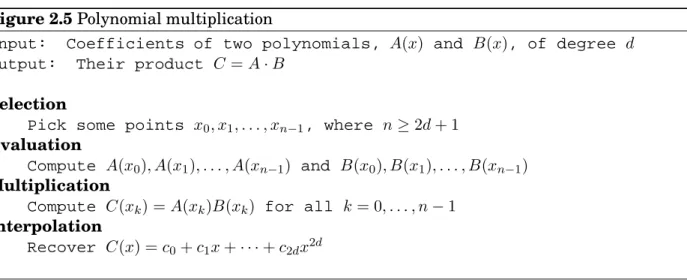
2.6.2 Evaluation by divide-and-conquer
Here’s an idea for how to pick thenpoints at which to evaluate a polynomial A(x) of degree ≤n−1. If we choose them to be positive-negative pairs, that is,
±x0,±x1, . . . ,±xn/2−1,
then the computations required for each A(xi) and A(−xi) overlap a lot, because the even powers ofxi coincide with those of−xi.
To investigate this, we need to splitA(x)into its odd and even powers, for instance 3 + 4x+ 6x2+ 2x3+x4+ 10x5 = (3 + 6x2+x4) +x(4 + 2x2+ 10x4). Notice that the terms in parentheses are polynomials inx2. More generally,
A(x) = Ae(x2) +xAo(x2),
where Ae(·), with the even-numbered coefficients, and Ao(·), with the odd-numbered coeffi-cients, are polynomials of degree ≤ n/2−1 (assume for convenience thatn is even). Given pairedpoints±xi, the calculations needed forA(xi)can be recycled toward computingA(−xi):
A(xi) = Ae(x2i) +xiAo(x2i) A(−xi) = Ae(x2i)−xiAo(x2i).
In other words, evaluating A(x) at n paired points ±x0, . . . ,±xn/2−1 reduces to evaluating
Evaluate: Adegree(x) ≤n−1 Ae(x)andAo(x) degree≤n/2−1 at: at: −x0 +x1 −x1 · · · · · · x2 0 −xn/2−1 +xn/2−1 x2 1 x2n/2−1 +x0 Equivalently, evaluate:
The original problem of size nis in this way recast as two subproblems of sizen/2, followed by some linear-time arithmetic. If we could recurse, we would get a divide-and-conquer pro-cedure with running time
T(n) = 2T(n/2) +O(n), which isO(nlogn), exactly what we want.
But we have a problem: The plus-minus trick only works at the top level of the recur-sion. To recurse at the next level, we need the n/2 evaluation pointsx2
0, x21, . . . , x2n/2−1 to be
themselvesplus-minus pairs. But how can a square be negative? The task seems impossible! Unless, of course, we use complex numbers.
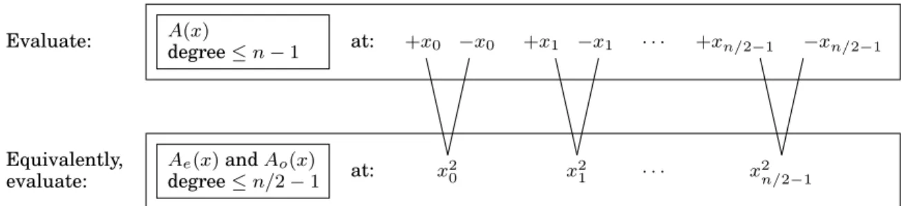
Fine, but which complex numbers? To figure this out, let us “reverse engineer” the process. At the very bottom of the recursion, we have a single point. This point might as well be1, in which case the level above it must consist of its square roots,±√1 =±1.
−1 −i −1 +1 +1 +i +1 .. .
The next level up then has±√+1 =±1as well as thecomplexnumbers±√−1 =±i, wherei is the imaginary unit. By continuing in this manner, we eventually reach the initial set ofn points. Perhaps you have already guessed what they are: thecomplexnth roots of unity, that is, thencomplex solutions to the equationzn= 1.
Figure 2.6 is a pictorial review of some basic facts about complex numbers. The third panel of this figure introduces thenth roots of unity: the complex numbers1, ω, ω2, . . . , ωn−1, where ω=e2πi/n. Ifnis even,
2. Squaring them produces the(n/2)nd roots of unity.
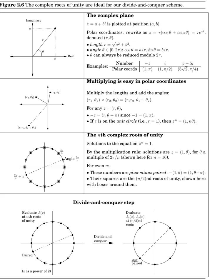
Therefore, if we start with these numbers for somenthat is a power of2, then at successive levels of recursion we will have the(n/2k)th roots of unity, fork = 0,1,2,3, . . .. All these sets of numbers are plus-minus paired, and so our divide-and-conquer, as shown in the last panel, works perfectly. The resulting algorithm is the fast Fourier transform (Figure 2.7).
Figure 2.6The complex roots of unity are ideal for our divide-and-conquer scheme. θ Real Imaginary a b r
The complex plane
z=a+biis plotted at position(a, b).
Polar coordinates: rewrite as z = r(cosθ+isinθ) = reiθ, denoted(r, θ).
•lengthr=√a2+b2.
•angleθ∈[0,2π):cosθ=a/r,sinθ=b/r.
•θcan always be reduced modulo2π.
Examples: Polar coordsNumber −1 i 5 + 5i
(1, π) (1, π/2) (5√2, π/4)
(r1r2, θ1+θ2)
(r1, θ1)
(r2, θ2)
Multiplying is easy in polar coordinates Multiply the lengths and add the angles:
(r1, θ1)×(r2, θ2) = (r1r2, θ1+θ2). For anyz= (r, θ),
• −z= (r, θ+π)since−1 = (1, π).
•Ifzis on theunit circle(i.e.,r= 1), thenzn= (1, nθ).
Angle2π n 4π n 2π n+π
Thenth complex roots of unity Solutions to the equationzn= 1.
By the multiplication rule: solutions arez = (1, θ), forθa
multiple of2π/n(shown here forn= 16).
For evenn:
•These numbers areplus-minus paired:−(1, θ) = (1, θ+π).
•Their squares are the(n/2)nd roots of unity, shown here
with boxes around them. Divide-and-conquer step Evaluate Ae(x), Ao(x) at(n/2)nd roots Still paired Divide and conquer Paired EvaluateA(x) atnth roots of unity (nis a power of 2)
Figure 2.7The fast Fourier transform (polynomial formulation)
function FFT(A, ω)
Input: Coefficient representation of a polynomial A(x)
of degree ≤n−1, where n is a power of 2 ω, an nth root of unity
Output: Value representation A(ω0), . . . , A(ωn−1)
if ω = 1: return A(1)
express A(x) in the form Ae(x2) +xAo(x2)
call FFT(Ae, ω2) to evaluate Ae at even powers of ω
call FFT(Ao, ω2) to evaluate Ao at even powers of ω
for j= 0 to n−1: compute A(ωj) =A
e(ω2j) +ωjAo(ω2j)
return A(ω0), . . . , A(ωn−1)
2.6.3 Interpolation
Let’s take stock of where we are. We first developed a high-level scheme for multiplying polynomials (Figure 2.5), based on the observation that polynomials can be represented in two ways, in terms of theircoefficientsor in terms of theirvaluesat a selected set of points.
Interpolation Coefficient representation a0, a1, . . . , an−1 Value representation A(x0), A(x1), . . . , A(xn−1) Evaluation
The value representation makes it trivial to multiply polynomials, but we cannot ignore the coefficient representation since it is the form in which the input and output of our overall algorithm are specified.
So we designed the FFT, a way to move from coefficients to values in time justO(nlogn), when the points{xi}are complexnth roots of unity (1, ω, ω2, . . . , ωn−1).
hvaluesi = FFT(hcoefficientsi, ω).
The last remaining piece of the puzzle is the inverse operation, interpolation. It will turn out, amazingly, that
hcoefficientsi = 1
nFFT(hvaluesi, ω
−1).
Interpolation is thus solved in the most simple and elegant way we could possibly have hoped for—using the same FFT algorithm, but called withω−1 in place ofω! This might seem like a miraculous coincidence, but it will make a lot more sense when we recast our polynomial oper-ations in the language of linear algebra. Meanwhile, ourO(nlogn)polynomial multiplication algorithm (Figure 2.5) is now fully specified.
A matrix reformulation
To get a clearer view of interpolation, let’s explicitly set down the relationship between our two representations for a polynomialA(x)of degree≤n−1. They are both vectors of nnumbers, and one is a linear transformation of the other:
A(x0) A(x1) ... A(xn−1) = 1 x0 x20 · · · xn0−1 1 x1 x21 · · · xn1−1 ... 1 xn−1 x2n−1 · · · xnn−−11 a0 a1 ... an−1 .
Call the matrix in the middle M. Its specialized format—a Vandermonde matrix—gives it many remarkable properties, of which the following is particularly relevant to us.
Ifx0, . . . , xn−1 are distinct numbers, thenM is invertible.
The existence ofM−1 allows us to invert the preceding matrix equation so as to express coef-ficients in terms of values. In brief,
Evaluation is multiplication byM, while interpolation is multiplication byM−1.
This reformulation of our polynomial operations reveals their essential nature more clearly. Among other things, it finally justifies an assumption we have been making throughout, that A(x)is uniquely characterized by its values at anynpoints—in fact, we now have an explicit formula that will give us the coefficients ofA(x)in this situation. Vandermonde matrices also have the distinction of being quicker to invert than more general matrices, inO(n2)time
in-stead ofO(n3). However, using this for interpolation would still not be fast enough for us, so once again we turn to our special choice of points—the complex roots of unity.
Interpolation resolved
In linear algebra terms, the FFT multiplies an arbitrary n-dimensional vector—which we have been calling thecoefficient representation—by then×nmatrix
Mn(ω) = 1 1 1 · · · 1 1 ω ω2 · · · ωn−1 1 ω2 ω4 · · · ω2(n−1) ... 1 ωj ω2j · · · ω(n−1)j ... 1 ω(n−1) ω2(n−1) · · · ω(n−1)(n−1) ←− row forω0= 1 ←− ω ←− ω2 ... ←− ωj ... ←− ωn−1
whereωis a complexnth root of unity, andnis a power of2. Notice how simple this matrix is to describe: its(j, k)th entry (starting row- and column-count at zero) isωjk.
Multiplication byM =Mn(ω)maps thekth coordinate axis (the vector with all zeros except for a1at positionk) onto thekth column ofM. Now here’s the crucial observation, which we’ll
Figure 2.8 The FFT takes points in the standard coordinate system, whose axes are shown here as x1, x2, x3, and rotates them into the Fourier basis, whose axes are the columns of
Mn(ω), shown here asf1, f2, f3. For instance, points in directionx1 get mapped into direction
f1. FFT x1 x3 x2 f3 f1 f2
prove shortly: the columns of M are orthogonal (at right angles) to each other. Therefore they can be thought of as the axes of an alternative coordinate system, which is often called the Fourier basis. The effect of multiplying a vector by M is to rotate it from the standard basis, with the usual set of axes, into the Fourier basis, which is defined by the columns of M (Figure 2.8). The FFT is thus a change of basis, arigid rotation. The inverse ofM is the opposite rotation, from the Fourier basis back into the standard basis. When we write out the orthogonality condition precisely, we will be able to read off this inverse transformation with ease:
Inversion formula Mn(ω)−1 = n1Mn(ω−1).
Butω−1 is also annth root of unity, and so interpolation—or equivalently, multiplication by Mn(ω)−1—is itself just an FFT operation, but withω replaced byω−1.
Now let’s get into the details. Takeωto bee2πi/nfor convenience, and think of the columns of M as vectors in Cn. Recall that the angle between two vectors u = (u0, . . . , un
−1) and
v= (v0, . . . , vn−1)inCnis just a scaling factor times theirinner product
u·v∗ = u0v0∗+u1v1∗+· · ·+un−1v∗n−1,
where z∗ denotes the complex conjugate4 ofz. This quantity is maximized when the vectors
lie in the same direction and is zero when the vectors are orthogonal to each other. The fundamental observation we need is the following.
Lemma The columns of matrixM are orthogonal to each other. Proof. Take the inner product of any columnsjandk of matrixM,
1 +ωj−k+ω2(j−k)+· · ·+ω(n−1)(j−k).
4Thecomplex conjugate of a complex numberz =reiθ isz∗ = re−iθ. The complex conjugate of a vector (or
This is a geometric series with first term1, last termω(n−1)(j−k), and ratioω(j−k). Therefore it evaluates to(1−ωn(j−k))/(1−ω(j−k)), which is0—except whenj=k, in which case all terms
are1and the sum isn.
The orthogonality property can be summarized in the single equation M M∗=nI,
since(M M∗)ij is the inner product of the ith and jth columns of M (do you see why?). This
immediately impliesM−1 = (1/n)M∗: we have an inversion formula! But is it the same for-mula we earlier claimed? Let’s see—the (j, k)th entry of M∗ is the complex conjugate of the
corresponding entry ofM, in other wordsω−jk. WhereuponM∗ =Mn(ω−1), and we’re done.
And now we can finally step back and view the whole affair geometrically. The task we need to perform, polynomial multiplication, is a lot easier in the Fourier basis than in the standard basis. Therefore, we first rotate vectors into the Fourier basis (evaluation), then perform the task (multiplication), and finally rotate back (interpolation). The initial vectors arecoefficient representations, while their rotated counterparts arevalue representations. To efficiently switch between these, back and forth, is the province of the FFT.
2.6.4 A closer look at the fast Fourier transform
Now that our efficient scheme for polynomial multiplication is fully realized, let’s hone in more closely on the core subroutine that makes it all possible, the fast Fourier transform. The definitive FFT algorithm
The FFT takes as input a vector a = (a0, . . . , an−1) and a complex number ω whose powers
1, ω, ω2, . . . , ωn−1 are the complexnth roots of unity. It multiplies vectoraby then×nmatrix Mn(ω), which has(j, k)th entry (starting row- and column-count at zero) ωjk. The potential for using divide-and-conquer in this matrix-vector multiplication becomes apparent whenM’s columns are segregated into evens and odds:
=
a Mn(ω) an−1 a0 a1 a2 a3 a4 .. . ωjk k j=
a2 a1 a3 an−1 .. . a0 .. . an−2 2k+ 1 Column 2k Even ω2jk ωj·ω2jkcolumns columnsOdd
j Rowj a2 a1 a3 an−1 .. . a0 .. . an−2 ω2jk ω2jk ωj·ω2jk 2k+ 1 Column j+n/2 2k −ωj·ω2jk
In the second step, we have simplified entries in the bottom half of the matrix usingωn/2 =−1
Figure 2.9The fast Fourier transform
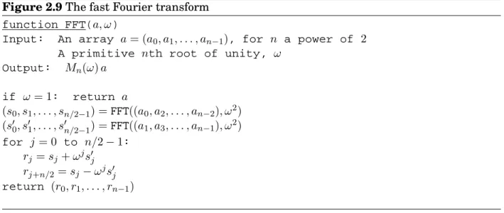
function FFT(a, ω)
Input: An array a= (a0, a1, . . . , an−1), for n a power of 2
A primitive nth root of unity, ω
Output: Mn(ω)a if ω = 1: return a (s0, s1, . . . , sn/2−1) =FFT((a0, a2, . . . , an−2), ω2) (s0 0, s01, . . . , s0n/2−1) =FFT((a1, a3, . . . , an−1), ω2) for j= 0 to n/2−1: rj =sj+ωjs0j rj+n/2=sj−ωjs0j return (r0, r1, . . . , rn−1)
bottom left. And the top and bottom right submatrices are almost the same as Mn/2(ω2), but with theirjth rows multiplied through byωj and−ωj, respectively. Therefore the final product is the vector
a0 a2 .. . an−2 a0 a2 .. . an−2 Mn/2 Mn/2 a1 a3 .. . an−1 a1 a3 .. . an−1 Mn/2 Mn/2 +ωj −ωj j+n/2 Rowj
In short, the product of Mn(ω)with vector (a0, . . . , an−1), a size-nproblem, can be expressed
in terms of two size-n/2 problems: the product of Mn/2(ω2) with (a0, a2, . . . , an−2) and with
(a1, a3, . . . , an−1). This divide-and-conquer strategy leads to the definitive FFT algorithm of
Figure 2.9, whose running time isT(n) = 2T(n/2) +O(n) =O(nlogn). The fast Fourier transform unraveled
Throughout all our discussions so far, the fast Fourier transform has remained tightly co-cooned within a divide-and-conquer formalism. To fully expose its structure, we now unravel the recursion.
The divide-and-conquer step of the FFT can be drawn as a very simple circuit. Here is how a problem of sizenis reduced to two subproblems of sizen/2 (for clarity, one pair of outputs (j, j +n/2)is singled out):
a0 a2 a3 j+n/2 j a1 an−1 rj+n/2 FFTn/2 FFTn/2 ... ... an−2 rj FFTn(input:a0, . . . , an−1, output:r0, . . . , rn−1)
We’re using a particular shorthand: the edges are wires carrying complex numbers from left to right. A weight ofjmeans “multiply the number on this wire byωj.” And when two wires come into a junction from the left, the numbers they are carrying get added up. So the two outputs depicted are executing the commands
rj = sj+ωjs0j rj+n/2 = sj−ωjs0j
from the FFT algorithm (Figure 2.9), via a pattern of wires known as abutterfly: .
Unraveling the FFT circuit completely for n= 8elements, we get Figure 10.4. Notice the following.
1. Forninputs there arelog2nlevels, each withnnodes, for a total ofnlognoperations. 2. The inputs are arranged in a peculiar order: 0,4,2,6,1,5,3,7.
Why? Recall that at the top level of recursion, we first bring up the even coefficients of the input and then move on to the odd ones. Then at the next level, the even coefficients of this first group (which therefore are multiples of 4, or equivalently, have zero as their two least significant bits) are brought up, and so on. To put it otherwise, the inputs are arranged by increasinglastbit of the binary representation of their index, resolving ties by looking at the next more significant bit(s). The resulting order in binary,000,100,010,110,001,101,011,111, is the same as the natural one,000,001,010,011,100,101,110,111 except the bits are mirrored!
3. There is a unique path between each inputaj and each outputA(ωk).
This path is most easily described using the binary representations of j and k (shown in Figure 10.4 for convenience). There are two edges out of each node, one going up (the0-edge) and one going down (the1-edge). To get toA(ωk)from any input node, simply follow the edges specified in the bit representation of k, starting from the rightmost bit. (Can you similarly specify the path in the reverse direction?)
4. On the path betweenaj andA(ωk), the labels add up tojk mod 8. Since ω8 = 1, this means that the contribution of input a
j to output A(ωk) is ajωjk, and therefore the circuit computes correctly the values of polynomialA(x).
5. And finally, notice that the FFT circuit is a natural for parallel computation and direct implementation in hardware.
Figure 2.10The fast Fourier transform circuit.
! "# $% &' () *+ ,-./
a
0a
4a
2a
6a
1a
5a
7A
(
ω
1)
A
(
ω
2)
A
(
ω
3)
A
(
ω
4)
A
(
ω
5)
A
(
ω
6)
A
(
ω
7)
a
3A
(
ω
0)
1 4 4 4 4 6 6 7 4 4 2 2 6 3 2 5 4 000 100 010 110 001 101 011 111 111 110 101 100 011 010 001 000The slow spread of a fast algorithm
In 1963, during a meeting of President Kennedy’s scientific advisors, John Tukey, a math-ematician from Princeton, explained to IBM’s Dick Garwin a fast method for computing Fourier transforms. Garwin listened carefully, because he was at the time working on ways to detect nuclear explosions from seismographic data, and Fourier transforms were the bot-tleneck of his method. When he went back to IBM, he asked John Cooley to implement Tukey’s algorithm; they decided that a paper should be published so that the idea could not be patented.
Tukey was not very keen to write a paper on the subject, so Cooley took the initiative. And this is how one of the most famous and most cited scientific papers was published in 1965, co-authored by Cooley and Tukey. The reason Tukey was reluctant to publish the FFT was not secretiveness or pursuit of profit via patents. He just felt that this was a simple observation that was probably already known. This was typical of the period: back then (and for some time later) algorithms were considered second-class mathematical objects, devoid of depth and elegance, and unworthy of serious attention.
But Tukey was right about one thing: it was later discovered that British engineers had used the FFT for hand calculations during the late 1930s. And—to end this chapter with the same great mathematician who started it—a paper by Gauss in the early 1800s on (what else?) interpolation contained essentially the same idea in it! Gauss’s paper had remained a secret for so long because it was protected by an old-fashioned cryptographic technique: like most scientific papers of its era, it was written in Latin.
Exercises
2.1. Use the divide-and-conquer integer multiplication algorithm to multiply the two binary integers
10011011and10111010.
2.2. Show that for any positive integersnand any baseb, there must some power ofblying in the
range[n, bn].
2.3. Section 2.2 describes a method for solving recurrence relations which is based on analyzing the recursion tree and deriving a formula for the work done at each level. Another (closely related) method is to expand out the recurrence a few times, until a pattern emerges. For instance, let’s start with the familiarT(n) = 2T(n/2) +O(n). Think ofO(n)as being≤cnfor some constantc,
so:T(n)≤2T(n/2) +cn. By repeatedly applying this rule, we can boundT(n)in terms ofT(n/2),
thenT(n/4), thenT(n/8), and so on, at each step getting closer to the value ofT(·)we do know,
namelyT(1) =O(1). T(n) ≤ 2T(n/2) +cn ≤ 2[2T(n/4) +cn/2] +cn = 4T(n/4) + 2cn ≤ 4[2T(n/8) +cn/4] + 2cn = 8T(n/8) + 3cn ≤ 8[2T(n/16) +cn/8] + 3cn = 16T(n/16) + 4cn ...
A pattern is emerging... the general term is
T(n)≤2kT(n/2k) +kcn.
Plugging ink= log2n, we getT(n)≤nT(1) +cnlog2n=O(nlogn).
(a) Do the same thing for the recurrenceT(n) = 3T(n/2) +O(n). What is the generalkth term
in this case? And what value ofkshould be plugged in to get the answer?
(b) Now try the recurrenceT(n) =T(n−1) +O(1), a case which is not covered by the master
theorem. Can you solve this too?
2.4. Suppose you are choosing between the following three algorithms:
• AlgorithmAsolves problems by dividing them into five subproblems of half the size,
recur-sively solving each subproblem, and then combining the solutions in linear time.
• AlgorithmBsolves problems of sizenby recursively solving two subproblems of sizen−1
and then combining the solutions in constant time.
• AlgorithmCsolves problems of sizenby dividing them into nine subproblems of sizen/3,
recursively solving each subproblem, and then combining the solutions inO(n2)time. What are the running times of each of these algorithms (in big-Onotation), and which would you
choose?
2.5. Solve the following recurrence relations and give aΘbound for each of them.
(a) T(n) = 2T(n/3) + 1
(c) T(n) = 7T(n/7) +n (d) T(n) = 9T(n/3) +n2 (e) T(n) = 8T(n/2) +n3 (f) T(n) = 49T(n/25) +n3/2logn (g) T(n) =T(n−1) + 2 (h) T(n) =T(n−1) +nc, wherec ≥1is a constant
(i) T(n) =T(n−1) +cn, wherec >1is some constant (j) T(n) = 2T(n−1) + 1
(k) T(n) =T(√n) + 1
2.6. A linear, time-invariant system has the following impulse response:
$% ! ("# $% &' () *+ ,- ./ t b(t) t0 1/t0
(a) Describe in words the effect of this system. (b) What is the corresponding polynomial?
2.7. What is the sum of thenth roots of unity? What is their product ifnis odd? Ifnis even?
2.8. Practice with the fast Fourier transform.
(a) What is the FFT of(1,0,0,0)? What is the appropriate value ofωin this case? And of which
sequence is(1,0,0,0)the FFT?
(b) Repeat for(1,0,1,−1).
2.9. Practice with polynomial multiplication by FFT.
(a) Suppose that you want to multiply the two polynomials x+ 1 andx2+ 1using the FFT. Choose an appropriate power of two, find the FFT of the two sequences, multiply the results componentwise, and compute the inverse FFT to get the final result.
(b) Repeat for the pair of polynomials1 +x+ 2x2and2 + 3x.
2.10. Find the unique polynomial of degree4that takes on valuesp(1) = 2,p(2) = 1,p(3) = 0,p(4) = 4,
andp(5) = 0. Write your answer in the coefficient representation.
2.11. In justifying our matrix multiplication algorithm (Section 2.5), we claimed the following block-wise property: ifX andY aren×nmatrices, and
X = A B C D , Y = E F G H .
whereA, B, C, D, E, F, G, and H are n/2×n/2 submatrices, then the product XY can be
expressed in terms of these blocks:
XY = A B C D E F G H = AE+BG AF+BH CE+DG CF+DH
Prove this property.
2.12. How many lines, as a function of n(in Θ(·) form), does the following program print? Write a
recurrence and solve it. You may assumenis a power of2.
function f(n) if n > 1:
print_line(‘‘still going’’) f(n/2)
f(n/2)
2.13. A binary tree is full if all of its vertices have either zero or two children. Let Bn denote the number of full binary trees withnvertices.
(a) By drawing out all full binary trees with3,5, or7vertices, determine the exact values of
B3,B5, andB7. Why have we left out even numbers of vertices, likeB4? (b) For generaln, derive a recurrence relation forBn.
(c) Show by induction thatBn isΩ(2n).
2.14. You are given an array ofnelements, and you notice that some of the elements are duplicates;
that is, they appear more than once in the array. Show how to remove all duplicates from the array in timeO(nlogn).
2.15. In our median-finding algorithm (Section 2.4), a basic primitive is the splitoperation, which takes as input an arrayS and a valuev and then divides S into three sets: the elements less
thanv, the elements equal tov, and the elements greater thanv. Show how to implement this
splitoperationin place, that is, without allocating new memory.
2.16. You are given an infinite arrayA[·]in which the firstncells contain integers in sorted order and
the rest of the cells are filled with∞. You arenotgiven the value ofn. Describe an algorithm that
takes an integerxas input and finds a position in the array containingx, if such a position exists,
inO(logn)time. (If you are disturbed by the fact that the arrayAhas infinite length, assume
instead that it is of lengthn, but that you don’t know this length, and that the implementation
of the array data type in your programming language returns the error message∞ whenever
elementsA[i]withi > nare accessed.)
2.17. Given a sorted array of distinct integers A[1, . . . , n], you want to find out whether there is an
indexifor whichA[i] =i. Give a divide-and-conquer algorithm that runs in timeO(logn).
2.18. Consider the task of searching a sorted arrayA[1. . . n]for a given elementx: a task we usually
perform by binary search in timeO(logn). Show that any algorithm that accesses the array only
via comparisons (that is, by asking questions of the form “isA[i]≤z?”), must takeΩ(logn)steps.
2.19. Ak-way merge operation.Suppose you haveksorted arrays, each withnelements, and you want
(a) Here’s one strategy: Using themergeprocedure from Section 2.3, merge the first two ar-rays, then merge in the third, then merge in the fourth, and so on. What is the time complexity of this algorithm, in terms ofkandn?
(b) Give a more efficient solution to this problem, using divide-and-conquer. 2.20. Show that any array of integersx[1. . . n]can be sorted inO(n+M)time, where
M = max
i xi−mini xi.
For smallM, this is linear time: why doesn’t theΩ(nlogn)lower bound apply in this case?
2.21. Mean and median.One of the most basic tasks in statistics is to summarize a set of observations {x1, x2, . . . , xn} ⊆Rby a single number. Two popular choices for this summary statistic are:
• The median, which we’ll callµ1 • The mean, which we’ll callµ2
(a) Show that the median is the value ofµthat minimizes the function
X i
|xi−µ|.
You can assume for simplicity thatnis odd. (Hint: Show that for anyµ6=µ1, the function decreases if you moveµeither slightly to the left or slightly to the right.)
(b) Show that the mean is the value ofµthat minimizes the function
X i
(xi−µ)2.
One way to do this is by calculus. Another method is to prove that for anyµ∈R, X i (xi−µ)2 = X i (xi−µ2)2+n(µ−µ2)2.
Notice how the function forµ2 penalizes points that are far fromµmuch more heavily than the function forµ1. Thusµ2tries much harder to be close toallthe observations. This might sound like a good thing at some level, but it is statistically undesirable because just a few outliers can severely throw off the estimate ofµ2. It is therefore sometimes said thatµ1 is a more robust estimator thanµ2. Worse than either of them, however, isµ∞, the value ofµthat minimizes the function
max
i |xi−µ|.
(c) Show thatµ∞ can be computed inO(n)time (assuming the numbersxi are small enough that basic arithmetic operations on them take unit time).
2.22. You are given two sorted lists of size m and n. Give an O(logm+ logn) time algorithm for
computing thekth smallest element in the union of the two lists.
2.23. An array A[1. . . n] is said to have a majority element if more than half of its entries are the
same. Given an array, the task is to design an efficient algorithm to tell whether the array has a majority element, and, if so, to find that element. The elements of the array are not necessarily from some ordered domain like the integers, and so there can be no comparisons of the form “is
A[i]> A[j]?”. (Think of the array elements as GIF files, say.) However youcananswer questions
(a) Show how to solve this problem inO(nlogn)time. (Hint: Split the arrayAinto two arrays A1andA2of half the size. Does knowing the majority elements ofA1andA2help you figure out the majority element ofA? If so, you can use a divide-and-conquer approach.)
(b) Can you give a linear-time algorithm? (Hint: Here’s another divide-and-conquer approach: • Pair up the elements ofAarbitrarily, to getn/2pairs
• Look at each pair: if the two elements are different, discard both of them; if they are the same, keep just one of them
Show that after this procedure there are at mostn/2elements left, and that they have a
majority element if and only ifAdoes.)
2.24. On page 66 there is a high-level description of the quicksort algorithm. (a) Write down the pseudocode for quicksort.
(b) Show that itsworst-caserunning time on an array of sizenisΘ(n2). (c) Show that itsexpectedrunning time satisfies the recurrence relation
T(n)≤O(n) + 1
n
nX−1 i=1
(T(i) +T(n−i)).
Then, show that the solution to this recurrence isO(nlogn).
2.25. In Section 2.1 we described an algorithm that multiplies two n-bit binary integersx andy in
timena, wherea= log
23. Call this procedurefastmultiply(x, y).
(a) We want to convert the decimal integer10n(a1followed bynzeros) into binary. Here is the algorithm (assumenis a power of2):
function pwr2bin(n) if n= 1: return 10102 else:
z=???
return fastmultiply(z, z)
Fill in the missing details. Then give a recurrence relation for the running time of the algorithm, and solve the recurrence.
(b) Next, we want to convert any decimal integerxwithndigits (wherenis a power of 2) into
binary. The algorithm is the following: function dec2bin(x)
if n= 1: return binary[x]
else:
split x into two decimal numbers xL, xR with n/2 digits each return ???
Herebinary[·]is a vector that contains the binary representation of all one-digit integers.
That is,binary[0] = 02,binary[1] = 12, up tobinary[9] = 10012. Assume that a lookup in binarytakesO(1)time.
Fill in the missing details. Once again, give a recurrence for the running time of the algo-rithm, and solve it.
2.26. Professor F. Lake tells his class that it is asymptotically faster to square ann-bit integer than to
multiply twon-bit integers. Should they believe him?
2.27. Thesquareof a matrixAis its product with itself,AA.
(a) Show that five multiplications are sufficient to compute the square of a2×2matrix.
(b) What is wrong with the following algorithm for computing the square of ann×nmatrix?
“Use a divide-and-conquer approach as in Strassen’s algorithm, except that in-stead of getting7subproblems of sizen/2, we now get5subproblems of sizen/2
thanks to part (a). Using the same analysis as in Strassen’s algorithm, we can conclude that the algorithm runs in timeO(nlog25).”
(c) In fact, squaring matrices is no easier than matrix multiplication. In this part, you will show that if n×n matrices can be squared in time S(n) = O(nc), then any two n
×n
matrices can be multiplied in timeO(nc).
i. Given twon×nmatricesAandB, show that the matrixAB+BAcan be computed in
time3S(n) +O(n2).
ii. Given twon×nmatricesX andY, define the2n×2nmatricesAandBas follows: A= X 0 0 0 andB= 0 Y 0 0 .
What isAB+BA, in terms ofX andY?
iii. Using (i) and (ii), argue that the productXY can be computed in time3S(2n) +O(n2). Conclude that matrix multiplication takes timeO(nc).
2.28. TheHadamard matricesH0, H1, H2, . . .are defined as follows: • H0is the1×1matrix
1
• Fork >0,Hkis the2k×2k matrix
Hk =
Hk−1 Hk−1
Hk−1 −Hk−1
Show that ifv is a column vector of lengthn = 2k, then the matrix-vector productH
kv can be calculated usingO(nlogn)operations. Assume that all the numbers involved are small enough
that basic arithmetic operations like addition and multiplication take unit time.
2.29. Suppose we want to evaluate the polynomialp(x) =a0+a1x+a2x2+· · ·+anxnat pointx. (a) Show that the following simple routine, known asHorner’s rule, does the job and leaves the
answer inz. z=an
for i=n−1 downto 0:
z=zx+ai
(b) How many additions and multiplications does this routine use, as a function ofn? Can you
find a polynomial for which an alternative method is substantially better?
2.30. This problem illustrates how to do the Fourier Transform (FT) in modular arithmetic, for exam-ple, modulo7.
(a) There is a numberωsuch that all the powersω, ω2, . . . , ω6are distinct (modulo7). Find this
ω, and show thatω+ω2+
· · ·+ω6= 0. (Interestingly, for any prime modulus there is such a number.)
(b) Using the matrix form of the FT, produce the transform of the sequence(0,1,1,1,5,2)
mod-ulo7; that is, multiply this vector by the matrixM6(ω), for the value ofωyou found earlier. In the matrix multiplication, all calculations should be performed modulo7.
(c) Write down the matrix necessary to perform the inverse FT. Show that multiplying by this matrix returns the original sequence. (Again all arithmetic should be performed modulo 7.) (d) Now show how to multiply the polynomialsx2+x+ 1andx3+ 2x
−1using the FT modulo 7.
2.31. In Section 1.2.3, we studied Euclid’s algorithm for computing thegreatest common divisor(gcd) of two positive integers: the largest integer which divides them both. Here we will look at an alternative algorithm based on divide-and-conquer.
(a) Show that the following rule is true.
gcd(a, b) = 2 gcd(a/2, b/2) ifa, bare even gcd(a, b/2) ifais odd,bis even gcd((a−b)/2, b) ifa, bare odd
(b) Give an efficient divide-and-conquer algorithm for greatest common divisor.
(c) How does the efficiency of your algorithm compare to Euclid’s algorithm ifaandbaren-bit
integers? (In particular, sincen might be large you cannot assume that basic arithmetic
operations like addition take constant time.)
2.32. In this problem we will develop a divide-and-conquer algorithm for the following geometric task. CLOSEST PAIR
Input:A set of points in the plane,{p1= (x1, y1), p2= (x2, y2), . . . , pn= (xn, yn)}
Output: The closest pair of points: that is, the pair pi 6= pj for which the distance betweenpiandpj, that is, q
(xi−xj)2+ (yi−yj)2, is minimized.
For simplicity, assume thatnis a power of two, and that all thex-coordinatesxiare distinct, as are they-coordinates.
Here’s a high-level overview of the algorithm:
• Find a valuexfor which exactly half the points havexi < x, and half havexi> x. On this basis, split the points into two groups,LandR.
• Recursively find the closest pair inLand inR. Say these pairs arepL, qL∈LandpR, qR∈R, with distancesdLanddRrespectively. Letdbe the smaller of these two distances.
• It remains to be seen whether there is a point inL and a point in R that are less than
distancedapart from each other. To this end, discard all points withxi< x−dorxi> x+d and sort the remaining points byy-coordinate.
• Now, go through this sorted list, and for each point, compute its distance to theseven sub-sequent points in the list. LetpM, qM be the closest pair found in this way.
• The answer is one of the three pairs{pL, qL},{pR, qR},{pM, qM}, whichever is closest. (a) In order to prove the correctness of this algorithm, start by showing the following property:
any square of sized×din the plane contains at most four points ofL.
(b) Now show that the algorithm is correct. The only case which needs careful consideration is when the closest pair is split betweenLandR.
(c) Write down the pseudocode for the algorithm, and show that its running time is given by the recurrence:
T(n) = 2T(n/2) +O(nlogn).
Show that the solution to this recurrence isO(nlog2n).