Meta-learning for time series forecasting and forecast
combination
Christiane Lemke and Bogdan Gabrys
Smart Technologies Research Centre, School of Design, Engineering and Computing, Bournemouth University, Poole House, Talbot Campus, Poole, BH12 5BB, UK, Phone:+44 1202 595298, Fax:+44 1202
595314, email: [clemke, bgabrys]@bournemouth.ac.uk
Abstract
In research of time series forecasting, a lot of uncertainty is still related to the task of selecting an appropriate forecasting method for a problem. It is not only the individ-ual algorithms that are available in great quantities; combination approaches have been equally popular in the last decades. Alone the question of whether to choose the most promising individual method or a combination is not straightforward to answer. Usu-ally, expert knowledge is needed to make an informed decision, however, in many cases this is not feasible due to lack of resources like time, money and manpower. This work identifies an extensive feature set describing both the time series and the pool of in-dividual forecasting methods. The applicability of different meta-learning approaches are investigated, first to gain knowledge on which model works best in which situation, later to improve forecasting performance. Results show the superiority of a ranking-based combination of methods over simple model selection approaches.
Key words: Forecasting, Forecast combination, Time series, Time series features,
Meta-learning, Diversity
1. Introduction
Time series forecasting has been a very active area of research since the 1950’s, with research on the combination of time series forecasts starting a few years later. During this time, many empirical studies on forecasting performance have been con-ducted to assess performance of the continuously growing numbers of available algo-rithms, for example in [41] and [32]. These studies however fail to provide consistent
results as to which actual method performs best, which is not surprising considering the variety in investigated time series forecasting problems. Robert J. Hyndman described the future challenges for time series prediction [35] in the following words:”Now it is
time to identify why some methods work well and others do not”.
But what is it that determines the success or failure of a forecasting model? The well-known no-free-lunch theorem, for example described in [48], states that there are no algorithms that generally perform better or worse than random when looking at all possible data sets. This implies, that no assumptions on the performance of an algorithm can be made if nothing is known about the problem that it is applied to. Of course, there will be specific problems for which one algorithm performs better than another in practice. In accordance to this, this work investigates approaches to relax the assumption that nothing is known about a problem by automatically extracting domain knowledge from a data, linking it to well-performing methods and drawing conclusions for a similar set of time series.
Traditionally, experts visually inspect time series characteristics and fit models ac-cording to their judgement. This work investigates an automatic approach, since a thorough time series analysis by humans is often not feasible in practical applications that process a large number of time series in very limited time.
A classic and straightforward classification for time series has been given by Pegels [36]. Time series can thus have patterns that show different seasonal effects and trends, both of which can be additive, multiplicative or non-existent. Gardner [19] extended this classification by including damped trends. Time series analysis in order to find an appropriate ARIMA model has been discussed since the seminal paper of Box and Jenkins [6]. Guidelines are summarised in [33] and rely heavily on visually examining autocorrelation and partial autocorrelation values of a series.
The idea of using characteristics of univariate time series to select an appropriate forecasting model has been pursued since the 1990’s. The first systems were rule based and built on a mix of judgemental and quantitative methods. Collopy and Armstrong use time series features to generate 99 rules [12] for weighting four different models; features were obtained judgementally, by both visually inspecting the time series and using domain knowledge. Adya et al. later modify this system and reduced the
neces-sary human input [1][2], yet did not abandon expert intervention completely. Vokurka et al. [46] extract features automatically to weight between three individual models and a combination in a rule-base that was built automatically, but required manual re-view of the outputs. Completely automatic systems have been proposed in [4], where a generated rule base selects between six forecasting methods. Discriminant analysis to select between three forecasting methods using 26 features is used in [40].
The phrase ”meta-learning” in the context of time series was first used in [38] and represents a new term for describing the process of automatically acquiring knowl-edge for time series forecasting model selection that was adopted from the general machine learning community. Two case studies are presented in [38]: In the first one, a C4.5 decision tree is used to link six features to the performance of two forecasting methods; in the second one, the NOEMON approach [25] is used for ranking three methods. The most recent and comprehensive treatment of the subject can be found in [47], where time series are clustered according to their data characteristics and rules generated judgementally as well as using a decision tree. The approach is then ex-tended to determine weights for a combination of individual models based on data
Year Authors Features Meta-learning
method Time Series Model pool 1992 Collopy and Armstrong [12] 18 (judge-mental)
rule base (judge-mental)
126 (M1)
exp. smoothing (Holt and Brown), random walk, lin-ear regression
1996 Vokurka et al. [46]
5 rule base (partly automatic)
126 (M1)
exp. smoothing (single and Gardner), structural and a combination of the three 1997 Arinze et al.
[4]
6 rule base 67 exp. smoothing (Holt and
Winter), adaptive filtering, three ”hybrids” of the previ-ous
1997 Shah [40] 26 discriminant analysis
203 (M1)
exp. smoothing (single and Holt-Winter), structural 2000 Adya et al. [2] 26 (mainly
automatic)
rule base (judge-mental)
3003 (M3)
exp. smoothing (Holt and Brown), random walk, lin-ear regression 2004 Prudencio and Ludermir [38] 6/7 decision tree / NOEMON 99/645 (M3)
exp. smoothing, neural net-work/random walk, Holt’s smoothing, auto-regressive 2009 Wang et al.
[47]
9 decision tree 315 random walk, smoothing, ARIMA, neural network Table 1: Time series model selection - overview of literature
characteristics. Table 1 summarises some facts about the related work presented here for better overview of approaches and methods used. The calculation of features and meta-learning method listed are implemented automatically if not otherwise stated.
Some time series features presented in this work are similar to the ones used in literature, but new and different features are introduced extending previous work pub-lished in [28]. In particular, features concerning the diversity of the pool of algorithms are included, which is facilitated by adding a number of popular forecast combination algorithms to the feature pool. In addition to the original question of which model to select, this work also tries to find evidence for features being useful for guiding the choice of whether to pick an individual model or a combination. In an initial ex-ploratory experiment, decision trees are generated to find evidence for the existence of a link between time series characteristics and the performance of models. Leaving aside the requirement for interpretable rules and recommendations, four meta-learning techniques are compared in another empirical experiment, assessing potential perfor-mance improvements.
The paper is structured as follows: Section two will present the underlying empiri-cal experiments and results. Section three begins treating the model selection problem as a classification task and describes an extensive number of time series characteristics which are necessary to link performances of algorithms to the nature of the time series. The different experiments using meta-learning techniques are evaluated in section four.
2. Performance of forecasting and forecast combination methods
This part of this work presents empirical experiments that provide the basis for further meta-learning analysis. Individual predictors are diverse, but are kept relatively simple and, more importantly, automatic. These methods perform often just as well as more complex methods [32], are more efficient in terms of computational requirements and also more likely to be employed in practical applications, especially when no expert advice is available.
2.1. Data sets
Two data sets both consisting of 111 time series have been used in this study; they were obtained from the NN3 [13] and NN5 [14] neural network forecasting
competi-tions. NN3 data includes monthly empirical business time series with 52 to 126 obser-vations, while the NN5 series are daily time series from cash machine withdrawals with 735 observations each. The competition task was to predict the next 18 or 56 obser-vations, respectively. While NN3 data did not need specific preprocessing, NN5 data included some missing values, which were substituted by taking the mean of the value of the corresponding weekday of the previous and the following week. The last 18 or 56 values of each series were not used for training the models to enable out-of-sample error evaluation.
2.2. Forecasting Methods
Available forecasting algorithms can be roughly divided into a few groups. Simple approaches are often surprisingly robust and popular, for example those based on expo-nential smoothing [20], [32]. Statisticians and econometricians tend to rely on complex ARIMA models and their derivatives [6]. The machine learning community mainly looks at neural networks, either using Multi-Layer-Perceptrons with time-lagged time series observations as inputs as, for example, in [49] and [16], or recurrent networks with a memory, see, for example, [26]. As not all of the algorithms provide native multi-step-ahead forecasting, some of them are implemented using two approaches: An iterative approach, where the last prediction is fed back to the model to obtain the next forecast, or a direct approach, wherendifferent predictors are trained for each of the 1 tonsteps ahead problem. The selection of models used in this work is presented in the next paragraphs.
2.2.1. Simple forecasting models
Many algorithms for forecasting time series are considered simple, yet they are usually very popular and can be surprisingly powerful. In the latest extensive M3 com-petitions [32], an exponential smoothing approach was considered a good match for the most successful complex method while providing a better trade-offbetween prediction accuracy and computational complexity. Simple methods used for this experimental study are listed below, where ˆyt+1 denotes the one-step-ahead prediction andyi the
• For themoving average, the arithmetic mean of the lastkobservations accord-ing to equation 1 is calculated. An appropriate time window is found by grid-searchingk-values from 1 to 20 and choosing thekwith the lowest mean squared error on a validation set prior to the test set.
ˆ yt+1= 1 k t X i=t−k+1 yi (1)
• Single exponential smoothingis the simplest representative of smoothing meth-ods and it is calculated by adjusting the previous forecast by the error it produced. The parameterαcontrols the extent of the adjustment and is determined again by minimising errors on a validation set that was separated from the training set.
ˆ
yt+1=αyt+(1−α)ˆyt (2)
• Taylor’s exponential smoothingis a more recently introduced exponential smoo-thing algorithm with a trend dampened by a factorφ, using a multiplicative ap-proach and a growth rateR[42]. It is given by equation 3, wherehis the number of periods ahead to be forecasted andltdenotes the estimated level of the series
at timet. The parametersαandβare smoothing constants taking values between zero and one, which are again determined by grid search.
ˆ yt+h = ltr Ph i=1φi t , lt = αyt+(1−α)(lt−1r φ t−1) (3) rt = β(lt/lt−1)+(1−β)rφt−1
• Polynomial regressionfits a polynomial to the time series by regressing time series indices against time series values. In this experiment, a suitable order of the polynome between two and six is grid-searched and the resulting curve extrapolated into the future; equation 4 shows the example of a regression of order three, whereωiare parameters estimated using the training set andtis the
ˆ
yt=ω0+ω1t+ω2t2+ω3t3 (4)
• The Theta-modelwas introduced in [5]. It decomposes series into short and long term components by applying a coefficientθto the second order differences of the time series, thus modifying the curvature of the time series. Here, it is employed using formulas given by [23]. The general equation for a theta-curve is
ˆ
yt+1(θ)=aˆt+bˆtt+θyt. (5)
Values ˆat and ˆbt are constants determined according to [23] andt is again the
time index. In the original setup in [5], two curves are used and the obtained forecasts averaged. The first forecast is calculated usingθ=0 which results in a linear regression problem where the linear part of formula 5 is extrapolated into the future. The second forecast forθ=2 is calculated using formula
ˆ yt+1(2)=α t−1 X i=0 (1−α)iyt−i(2)+(1−α)ny1(2), (6) which is a single exponential smoothing applied to seriesyt(2)
2.2.2. Automatic Box-Jenkins Models
Autoregressive integrated moving average models (ARIMA) according to [6] are a complex tool of modelling and forecasting time series. They are described by the notation ARIMA (p,d,q) and consist of the following three parts:
• AR(p) denotes the autoregressive part of order p. Autoregression defines a re-gressionyt=ω0+ω1yt−1+...ωpyt−p+twhere the target variable depends onp
time-lagged values of itself weighted by weightsωi.
• I(d) defines the degree of differencing involved. Differencing is a method of removing non-stationarity in a time series by calculating the change between each observation. The first difference of a time series is thus given by y0
t =
• MA(q) indicates the order of the moving average part of the model, which is given as a moving average of the error series. It can be described as a regression against the past error values of the seriesyt=ω0+ω1t−1+...ωqt−q+t
The identification of an appropriate ARIMA model for a specific time series is not straightforward [33] and usually involves expert knowledge and intervention. Two automatic approaches have been implemented for this study:
• The original time series as well as two series representing its first and second dif-ferences are submitted to the automatic ARMA selection process of a MATLAB toolbox published in [15], subsequently choosing the approach that produced the lowest MSE on the validation set. The maximum number of time lags used is an input parameter of the toolbox and has been set to two, which is sufficient in practice according to [33]. Furthermore, the same authors state, that it is almost never necessary to generate more than second-order differences of a time series, because data usually only involves nonstationarity of the first or second level.
• An alternative automatic approach for ARMA-modelling is included in the State-Space-Models Toolbox [37]. In this case, an appropriate order forpandqwas chosen using the Akaike’s Information criterion (AIC), while a suitable order of differencing was determined by the log-likelihood of a model given the corre-sponding differenced series.
2.2.3. Structural time series
The structural approach formulates a time series as a number of directly inter-pretable components such as trends or cycles. Structural models fit into the statistical framework of state space models, which allows usage of well established algorithms like the Kalman filter and Kalman smoother [22]. The State-Space-Models Toolbox [37] has been used for implementation of a local level model with a dummy seasonal component of either twelve or seven, depending on the data set used. A basic local level consists of a random walk with noise as described by the following formulas:
yt = µt+t, t∼NID(0, σ2) (7)
wheret andηtare normally and independently distributed error terms. Variable
µtrepresents a stochastic trend component in the more general structural time series
definition, for the random walk it simply denotes last time series observations.
2.2.4. Computational Intelligence models
Looking at the pool of available methods belonging to computational intelligence models, it is neural networks that have most frequently and successfully been used for forecasting purposes. An extensive summary of work done in this area can be found in [49], which is somewhat outdated but still very relevant in terms of guidelines given. According to these, a feed-forward neural network was implemented. It has one hidden layer with twelve neurons, training is carried out with a backpropagation algorithm with momentum. Input variables were the latest observations up to a lag of seven or twelve to catch weekly or yearly seasonality depending on the data set used. Ten neural networks have been trained and their predictions averaged to obtain the final forecasts.
Furthermore, a recurrent neural network of the Elman-type has been employed. There seem to be no general guidelines in literature about the architecture of a recurrent network for time series forecasting, but one thing seems to be a common agreement: They need more hidden nodes than the feedforward neural network because the tempo-ral relationship has to be modelled as well. In these experiments, the number of hidden nodes was set to 24 (double the amount of hidden nodes for the feedforward network).
2.3. Forecast Combinations
Combinations of forecasts are motivated by the fact that all models of a real world data generation process are likely to be misspecified and picking only one of the avail-able models is risky, especially if the data and consequently the performance of models change over time. It is a reliable method of decreasing model risk and aims at improv-ing forecast accuracy by exploitimprov-ing the different strengths of various models while also compensating their weaknesses. The following methods have been implemented for the experiments here:
• Usingsimple average, all available forecasts are averaged, which has proven to be a successful and robust method ([43]).
• Thesimple average with trimmingaverages individual forecasts as well, but without taking the worst performing 20% of the models into account. This is in accordance with guidelines given in [24], where 10-30% are recommended.
• In thevariance-based model, weights for a linear combination of forecasts are determined using past forecasting performance according to [34].
• The outperformance method was proposed in [10] and determines weights based on the number of times a method performed best in the past.
• Invariance-based pooling, past performance is used to group forecasts into two or three clusters by a k-means algorithm as suggested by Aiolfi and Timmermann in [3]. Forecasts of the historically better performing cluster are then averaged to obtain a final forecast.
Literature in the area of nonlinear forecast combination is quite sparse, which is probably due to the lack of evidence of success as stated in [43]. Only linear combina-tions are considered here.
2.4. Results
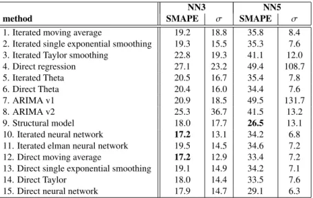
The following tables present result averages of the individual and combined meth-ods for the two data sets. The symmetric mean absolute percentage error (SMAPE) has been used for evaluating and comparing methods. It is a relative error measure that enables comparisons between different series and also comparison with the results of the forecasting competitions that provided the data sets. It is given by
SMAPE= 1 n n X t=1 |yt−yˆt| (yt+yˆt)/2 ∗100, (9)
wherendenotes the forecasting horizon. The standard deviation for each method is given to provide a measure of variability across the different time series.
Concerning individual methods in the NN3 competition in table 2, the feedforward neural networks perform quite well, together with the direct moving average. For the NN5 competitions, results in general are considerably worse, which can be attributed to the the longer period to be forecasted, where errors can accumulate quite quickly. The
NN3 NN5
method SMAPE σ SMAPE σ
1. Iterated moving average 19.2 18.8 35.8 8.4 2. Iterated single exponential smoothing 19.3 15.5 35.3 7.6 3. Iterated Taylor smoothing 22.8 19.3 41.1 12.0 4. Direct regression 27.1 23.2 49.4 108.7 5. Iterated Theta 20.5 16.7 35.4 7.8 6. Direct Theta 20.4 16.0 34.4 7.6 7. ARIMA v1 20.9 18.5 49.5 131.7 8. ARIMA v2 25.3 36.7 41.5 13.2 9. Structural model 18.0 17.7 26.5 13.1
10. Iterated neural network 17.2 13.1 34.2 6.8 11. Iterated elman neural network 19.5 14.5 34.6 7.2 12. Direct moving average 17.2 12.9 33.4 7.2 13. Direct single exponential smoothing 19.1 14.9 34.2 7.1
14. Direct Taylor 18.0 14.4 33.5 7.6
15. Direct neural network 17.9 14.7 29.1 6.3
Table 2: Performances averaged per data set and standard deviations for forecasting methods, best SMAPE printed in bold.
local level model with seasonality is the clear-cut winner here, closely followed by the direct neural network. ARIMA models suffer from outliers indicated by high standard deviation values and can only be fitted well in some cases. The three-cluster pooling approach outperforms the best individual method in both data sets, as can be observed in table 3 and has also been shown in previous work [29]. If this approach would have been submitted to the original NN3 competition, it would have ranked sixth out of 26 participants. The result for the NN5 competition looks less convincing, where it would have ranked 12th out of 20 participants. This shows that the longer series might require more complex algorithms due to their length and complexity.
NN3 NN5
method SMAPE σ SMAPE σ
1. simple average 17.5 13.8 32.2 7.2 2. simple trimmed average 17.4 13.6 31.8 7.1 3. outperformance 16.6 12.4 29.5 6.9 4. variance-based 18.1 13.2 26.5 6.8 5. pooling (2) 16.4 12.1 29.0 9.7 6. pooling (3) 16.8 12.3 25.7 10.5
7. regression 20.4 32.5 27.5 12.3
Table 3: Performances averaged per data set and standard deviations for combination methods, best SMAPE printed in bold.
1 2 3 4 5 6 7 8 9 10 11 12 13 14 15 0 5 10 15 20 25 method number
number of time series for which a method performed best
1 2 3 4 5 6 7 0 5 10 15 20 25 30 35 40
number of time series for which a method performed best
method number
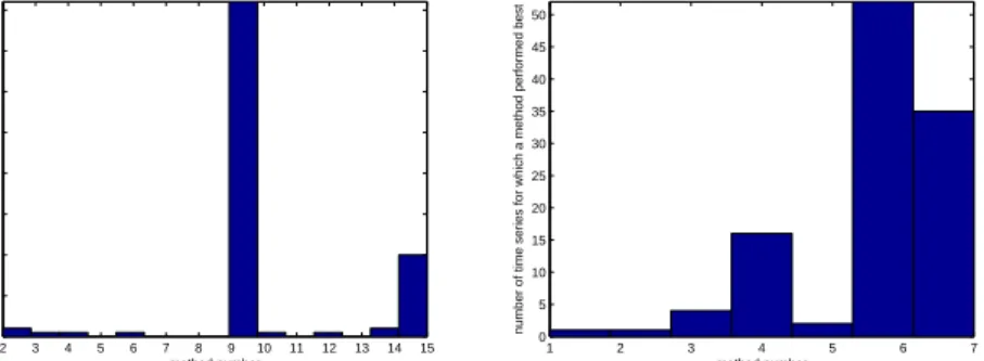
Figure 1: Histogram showing the number of times a particular method performs best for the NN3 data, left: individual methods, right: combinations
A look at the histograms of the best performing methods in figures 1 and 2 show some interesting facts as well: While the best performing individual methods are well spread on the NN3 data set, it is almost only the structural model and the direct neural network that perform best for NN5. Simple average combinations consequently per-form badly on the NN5 data set, as there are many predictors that comparatively do not perform well. The regression combination does not have an outstanding average performance, but performs best for the largest number of the individual series. This illustrates why it might be beneficial to identify conditions in which one or the other method is more likely to perform well, which will be investigated in the next sections.
2 3 4 5 6 7 8 9 10 11 12 13 14 15 0 10 20 30 40 50 60 70 80
number of time series for which a method performed best
method number 1 2 3 4 5 6 7 0 5 10 15 20 25 30 35 40 45 50 method number
number of time series for which a method performed best
Figure 2: Histogram showing the number of times a particular method performs best for the NN5 data, left: individual methods, right: combinations
3. Creating a feature pool
In the next step, the question of which individual forecasting method or combina-tion to choose for which time series will be treated as a classificacombina-tion problem. This requires the extraction of a number of features from the available time series, which will be discussed in this section. Finding suitable time series features for classification is not straightforward, as time series analysis is a complex area of research in itself [11]. The features used in this work were selected for their automatic detectability and their diversity and, as a group, aim to describe the nature of a time series as accurately as possible. Features describing diversity of the pool of individual methods have been added to provide information possibly relevant to combining approaches. This section introduces different groups of features before summarising them in a table within each paragraph.
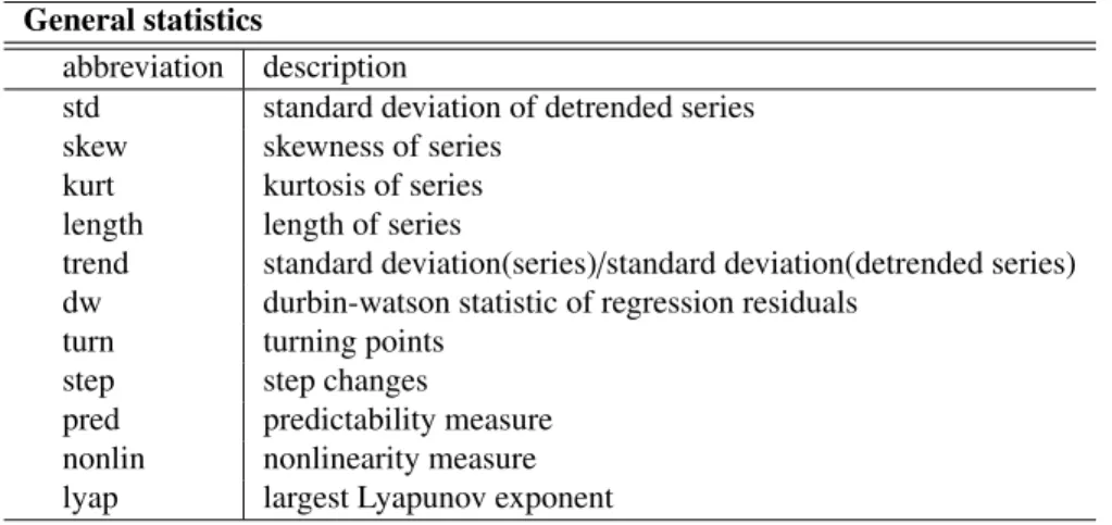
3.1. General statistics
For calculation of some of the descriptive statistics, the original time series has been detrended using a polynomial regression of up to order three. The residuals of this regressioneare then subjected to a Durbin-Watson test that checks their autocorrelation with the formula
d= P t(et−et−1)2 P te2t . (10)
General descriptive statistics in the feature set are standard deviation, skewness and kurtosis of the detrended series as well as its length. The quotient of the standard deviation of the original and the detrended series is calculated to provide a measure of how much of the variability of the series can be accounted for with the trend curve.
Turning points and step changes are adapted from [40], to capture oscillating be-haviour and structural breaks, respectively. A turning point for series with observa-tionsyi = {y1...yt}is given ifyiis a local maximum or minimum for its two closest
neighbours. A step change is counted whenever yi− {y1...yi−1} >2σ(y1...yi−1), where
{y1...yt−1}is the mean andσ(y1...yi−1) the standard deviation of the series up to point
i−1. Both measures are divided by the number of observations to ensure comparability. Two measures of interest have been published in [21]: The deterministic compo-nent of a time series measure is measured by representing a time series as a number of
delay vectors of embedding dimensionm, denoted byyt =[yt−1...yt−m].Delay vectors
are grouped according to their similarity, so that the variances of the targets provides an inverse indication of predictability. Furthermore, nonlinearity is estimated by gen-erating surrogate time series as the realisation of the null hypothesis that the series is linear. If the delay vector representations of original and surrogate series are signifi-cantly different, the time series is considered to be nonlinear.
General statistics
abbreviation description
std standard deviation of detrended series
skew skewness of series
kurt kurtosis of series
length length of series
trend standard deviation(series)/standard deviation(detrended series) dw durbin-watson statistic of regression residuals
turn turning points
step step changes
pred predictability measure
nonlin nonlinearity measure
lyap largest Lyapunov exponent
Table 4: Feature Pool - general statistics
The largest Lyapunov exponent is a measure for the separation rate of state-space trajectories that were initially close to each other and quantifies chaos in a time series. The average of the Lyapunov exponents calculated using software provided in [44] was added to the feature set.
3.2. Frequency domain
A number of features have been extracted from the fast fourier transform of the detrended series. The frequencies at which the three maximum values of the power spectrum occur are intended to give an indication of seasons and cycles, the maximum value of the power spectrum should give an indication of the general strength of the strongest seasonal or cyclic component. The number of peaks in the power spectrum that have a value of at least 60% of the maximum value quantify how many strong recurring components the time series has.
Frequency domain
abbreviation description
ff[1-3] power spectrum frequencies of three biggest values
ff[4] power spectrum: maximal value
ff[5] number of peaks not lower than 60% of the maximum
Table 5: Feature pool - frequency domain
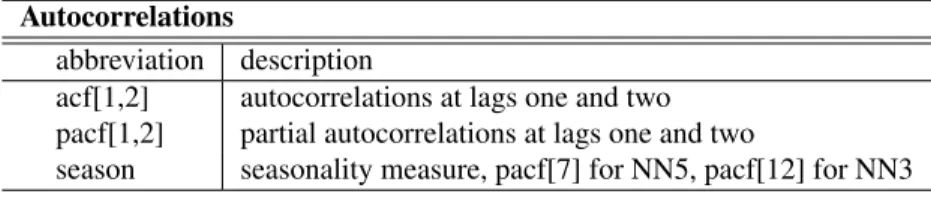
3.3. Autocorrelations
Autocorrelation and partial autocorrelation give indications on stationarity and sea-sonality of a time series; both of the measures have been included for the lags one and two. Furthermore, domain knowledge on seasonality is exploited by including partial autocorrelation of lag 12 for the NN3 data set which consists of monthly data and the partial autocorrelation of lag 7 for the NN5 data, which consists of weekly time series.
Autocorrelations
abbreviation description
acf[1,2] autocorrelations at lags one and two pacf[1,2] partial autocorrelations at lags one and two
season seasonality measure, pacf[7] for NN5, pacf[12] for NN3
Table 6: Feature pool - autocorrelations
3.4. Diversity features
When dealing with combinations of forecasts, it is crucial to look at characteristics of the available individual forecasts. It is desirable to have a diverse pool of individual predictors, ideally with the strengths of one forecast compensating weaknesses of an-other. Additionally, if there is one extremely superior forecast in the pool of available methods, it is unlikely that it will be outperformed in a combination with other fore-casts. Diversity is a well known concept in ensemble learning, which is a term normally used to describe strategies for training a number of models sharing the same functional approach. A few concepts have been successful in this area, for example bagging [8], boosting [17] or negative correlation learning [30]. However, since the predictors used here are also diverse in their functional approach and most of them cannot be ”trained” in a machine-learning fashion, these concepts are not applicable.
The standard ways to look at diversity for a number of methods is examining cor-relation coefficients. The feature pool here includes mean and standard deviation of the error correlation coefficients of the forecast pool. Other diversity measures have mainly been discussed in the context of classification tasks, for example in [27] and [18]. One of the few publications dealing with diversity in a regression context is [9], where an error functionefor training regression ensembles is introduced following the formula e= 1 M X i (ˆyi−y)2−κ∗ 1 M X i (ˆyi−y¯ˆ)2, (11)
where ˆyidenotes the prediction of theith ofMmodels,ythe actual observation and
¯ˆ
ythe mean of the output of all ensemble members. It has been shown, that the first term of this equation contains the bias and variance error terms, while the second error term includes the covariance of the ensemble members in addition to these. Hence, parameterκcontrols the extent of the covariance impact on the error. To exploit these findings in form of time series features, two values have been added to the feature set: The proposed error measure in its original form and the quotient of the mean error (first term of equation) and the variability between the members in the method pool (second term). In this way, the trade offbetween individual accuracy and diversity can be measured.
Diversity features
abbreviation description
div1 mean(SMAPEs)-mean(SMAPEs deviation from average SMAPE)
div2 mean(SMAPEs)/mean(SMAPEs deviation from average SMAPE)
div3 mean(correlation coefficients in the method pool) div4 std(correlation coefficients in the method pool) div5 number of methods in top performing cluster div6 distance top performing cluster to second best
Table 7: Feature pool - diversity
The clustering combination method inspires a different approach on quantifying diversity. A k-means clustering algorithm is used to group individual forecasts in three groups. The number of methods in the top performing cluster is then taken as a feature,
that will identify if there are few or many equally well performing methods, or even just a single one. Additionally, the distance of the mean of the top performing cluster to the mean of the second best is added, to put the two performances into relation.
4. Meta-learning
According to [45], the goal of meta learning is to”..understand how learning
it-self can become flexible according to the domain or task under study.” There have
been different more detailed interpretations of the term in the literature; in this work, meta-learning is referred to as the process of linking knowledge on the performance of so-called base-learners to the characteristics of the problem [39]. One difference to general perception of meta-learning is that the base-learners used here are not nec-essarily machine learning algorithms, but include other approaches as well. Many meta-learning approaches are available as reviewed in [45]; this section presents three different experiments: In the first step, decision trees using meta-features described in the previous section have been built as a machine learning method giving readable results. The second experiment compares a number of approaches and evaluates pos-sible performance improvements. In the last part of this section, performance of one approach is tested under competition conditions for the NN5 data set.
4.1. Experiment one - decision trees for data exploration
Decision trees were built using the Matlab statistics toolbox, choosing the minimum-cost-tree after a ten-fold crossvalidation. Features were determined on the whole time series, as the nature of this work is exploratory. Using all available methods as class labels did not yield interpretable results, which is why, concentrating on the best per-forming approaches in the underlying experiments, the classification problem has been reduced to three different questions:
• When does an individual method perform better, when a combination, when does it not matter? (three class labels)
• When should a structural model, a direct neural network, a pooling combination or a regression combination be used? (four class labels)
• How to decide between pooling and regression for the combination models? (two class labels)
Results given in this section do not claim to be universally applicable, they merely provide an insight on the existence of rules for the specific data set used. However, if the meta-features describe the series well and a series with similar characteristics can be found, it is probable that the guidelines are generalisable, but there is, of course, no guarantee.
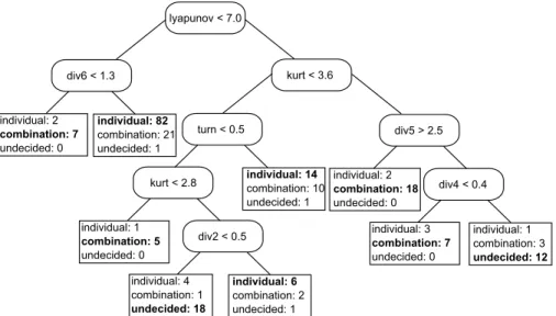
In the figures given in the following results, the leaf to the left of a node represents the data that fulfils its condition, the leaf to the right hand side represents data that does not. The numbers following the methods in the leafs denote the number of times this particular method performed best on the data subset. The first classification problem concerned the use of combinations and individual methods; the generated tree can be seen in Figure 5.
Figure 3: Decision tree 1
The first node of the tree divides the series into more and less chaotic series, indi-cated by the Lyapunov exponent. The majority of the less chaotic series to the left of the tree are best treated with an individual model, combination models are only suggested for series where the first and second best performing cluster do not have a huge
perfor-mance difference. Looking at the right part of the tree, three more diversity measures appear in the nodes together with the kurtosis and the turning point measure. Results include, amongst others, the suggestion that individual models should not be used for series with a high kurtosis, and for these a combination method is likely to perform well if the number of well performing methods is high or correlation coefficients are similar, otherwise, they tend to perform just as well as an individual model. The whole tree misclassifies 53 of the 222 data instances, which equals to a rate of 23% as op-posed to a misclassification rate of 49% when picking the class with the most training examples (individual method).
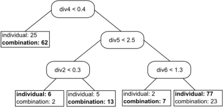
The same experiment was run only using features from the diversity feature set, to see how especially these affect combination performance. Additionally, the class label ”undecided” was replaced with combinations: As they have the reputation for being less risky, it seems like a straightforward approach to pick them whenever their performance is equal or better in comparison to individual methods.
Figure 4: Decision tree 2
In the top node of the tree given in figure 4, instances with a smaller variability in correlation coefficients (diversification measure four) are sent to the left side of the tree, where combination methods work best. This is counter-intuitive, as a bigger di-versity in individual forecasts should favour combinations, it however illustrates the fact that diversity has to be traded offwith individual accuracy and is not beneficial for combinations at all times. In the right part of the tree, most of the instances fall in rightmost leaf, which suggests individual approaches for individual pools with more
than two methods in the top performing cluster and a big distance between this cluster and the second best. Diversity measure two, the quantification of the actual trade-off between individual accuracy and diversity is another node of the subtree, claiming that if diversity is big in relation to individual accuracy (small value of the measure), an individual method should be used, and combinations otherwise. The misclassification rate of the tree is 26%, which is worse compared to the previous tree, indicating that the diversity features do not work optimally on their own. However, it is still considerably better than the rate of 49% that is obtained when just picking individual methods.
The second classification problem deals with the decision between the two best individual (structural model, neural network) and the two best combination models (pooling, regression), producing the tree shown in Figure 5.
Figure 5: Decision tree 3
The first node sends instances with three or fewer methods per cluster to a leaf sug-gesting to use a structural model. This shows, that the structural model will most likely be among the top three methods of the top performing cluster with such a superior performance that neither the neural network nor the combinations can beat. Structural models are also recommended for higher autocorrelation values at lag two. Pooling
performs well in the middle subtree, if the series only shows a low seasonality or if there are many well performing methods. Neural networks are suggested for in a con-figuration where other predictors have a higher individual accuracy compared to their diversity. This tree misclassifies 37% of the instances compared to 50% that would be misclassified using the most frequently appearing class label.
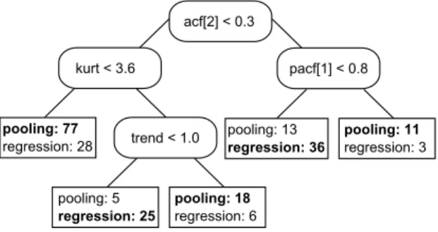
The third problem investigated is how to decide between using a pooling or a re-gression combination approach, the corresponding tree can be found in Figure 6. The features selected here differ from the ones selected in the previous experiment, and the tree is not easily interpretable. However, it misclassifies only 24% compared to 44% that would be misclassified in only using the pooling approach.
Figure 6: Decision tree 4
4.2. Experiment two - comparing meta-learning approaches
In this experiment, a number of machine learning algorithms for meta learning have been tested adopting the leave-one-out methodology that has, for example, been applied in [38]. Of the 222 series, only 221 are used as a training set before the remain-ing one is used to test the resultremain-ing meta-model. This process is repeated 222 times, until every series has been the test series once. To move away from the exploratory nature of the previous experiments, features for the test series were now only calcu-lated using the training set, which means that the last 18 or 56 observations were held back from the series. For the diversity features of the test series, only the validation set forecasts were used.
dealing with the classification problem of linking time series features to the class label of one of the most promising forecasting algorithms including the structural model, the direct neural network, variance-based pooling and the regression combination as investigated in the second problem of the last section. Three algorithms have been implemented:
• A feedforwardneural networkwith one hidden layer and 30 hidden nodes,
• adecision treeobtained by picking the minimum cost tree after a ten-fold cross validation and
• a support vector machine with a radial basis function as kernel function.
Only selecting one model that is applied to a problem as in the three more tradi-tional meta-learning approaches presented above has the obvious limitation of bearing a certain risk, even if one of the selected algorithms is a combination of predictors as in the case of our experiments. A newer approach that facilitates combinations on a higher level, the meta learning level, is presented in [7] and applied to time series forecasting in [31]. It allows taking relations of individual performances into account by providing a ranking of methods for a particular problem. The problem space is di-vided using clustering on a distance measure that was calculated using the time series features. Details of this so-called zoomed ranking and our implementation of it follow. In the first step of the zoomed ranking algorithm, distances in the set of time series are calculated. With the normalised features fx, where xis the meta-attribute number,
the distance of two series is given by the unweightedL1norm:
dist(si,sj)= X x fx,si−fx,sj maxk,i(fx,sk)−mink,i(fx,sk) (12)
The distances are then clustered using the k-means algorithm, and the series in the cluster closest to the test series are identified for further inspection. The ranking is then generated by a variation of the Adjust Ratio of Ratios (ARR), which is applied in a classification context in the original paper [7] and extended by a penalty for time intensity in [31], however, in this experiment, the time dimension was discarded and
the SMAPE measure was used instead of classifier success rates to adapt the ranking to regression problems. The pairwise ARR for modelsmpandmqon seriessiis
ARRsimp,mq= S MAPEmq
S MAPEmp
. (13)
A high ARR indicates that model p performs better than model q. To aggregate all rankings over the selected series and the pairwise ranking to one number per method, the following formula is used:
ARRmp = P mq n q Q siARR si mp,mq m (14)
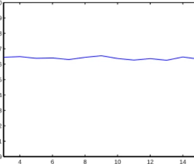
The method with the best ranking then gets selected, or, in an alternative approach, the rankings are then used to calculate convex weights for the four algorithms consid-ered in this experiment. One of the open questions using this approach is determining the number of clusters to use for the k-means algorithm. However, trying different val-ues for the number of clusters, it becomes clear that the impact on the performance is small as can be seen in figure 7, so that it is safe to set the number arbitrarily, within reason. 4 6 8 10 12 14 19 19.1 19.2 19.3 19.4 19.5 19.6 19.7 19.8 19.9 20
Figure 7: Average performance in relation to number of clusters
Performance results of all of the approaches presented in this section can be found in table 4.2. Experiments were run on the whole data set, but results are given sep-arately for the NN3 and the NN5 competition, to allow better comparison with the performances given in section two. However, it has to be stated that the performances
given in the table cannot be compared to the competition results, as the whole time series were used in the training set for building the models. The ranking approach combining four methods outperforms all other meta-learning approaches and also im-proves upon the best individual predictors. It can thus be seen, that combinations of models outperformed model selection on a meta-learning level, which underlines the need for approaches that provide a ranking of models as opposed to just recommending one of the available approaches.
Method NN3 NN5
neural network 17.0 27.3
decision tree 18.0 26.5
support vector machine 18.0 26.5
zoomed ranking, best method 17.5 26.6 zoomed ranking, combination 15.5 23.8
Table 8: Performances applying different meta-learning techniques
4.3. Experiment 3 - simulating NN5 competition conditions
For the last experiments, time series observations that were not yet available at the time of the competition were used for training the meta-models. In this experiment, the zoomed ranking approach presented in the previous section was evaluated on fea-tures that were calculated excluding the test data, hence the obtained forecast could have participated in the competition. This caused problems for the NN3 data set, as the necessary validation periods for the combination approaches would reduce the obser-vations available for individual model building to only 15 for the shortest of the series, which is too few for some of the methods to work. This experiment therefore only considers the NN5 competition.
Applying the zoomed ranking approach, the resulting out-of-sample SMAPE of 23.8 is similar to the performance in the previous experiment, showing that the ap-proach was successful also in competition conditions and improving the twelfth rank of the best individual method to rank nine of twenty competitors.
5. Conclusions
This work investigated meta-learning for time series prediction with the aim to link problem-specific knowledge to well performing forecasting methods and apply them in similar situations. Initially, an extensive pool of features for describing the nature of time series was identified. Along with features that have been used in previous publi-cations, several new ones have been added, for example a measure for nonlinearity and predictability and characteristics of the frequency spectrum. Furthermore, measures have not only been calculated for the time series themselves, but also for describing the behaviour of the pool of available individual forecasting methods. In that way, the following characteristics could be quantified: diversity in the method pool, the trade-offbetween individual accuracy and diversity, the size of the group of best performing individual methods and the distance to the group of second best performing methods.
Decision trees have been built to gain knowledge which of the chosen features are important for method selection. Some time series characteristics that lead to good re-sults in previous work did not seem to be significant for the time series and methods used here. However, the newly introduced diversity measures gave some interesting in-sights, quantifying some intuitive perceptions on mechanisms that make a combination more successful. One of the lessons that has been illustrated quite well is that diversity alone is not the key to a successful combination of methods, it is individual accuracy as well. Other easily interpretable results for the given data set include that individual methods in general work better on less chaotic time series and the pooling approach in particular works well if there are many well performing methods with a good ratio of accuracy and diversity in the method pool. It is not claimed that all of these guidelines are universally applicable to all data sets, however, it was shown that they do exist and can be successfully exploited for meta-learning experiments as illustrated in the other empirical experiments.
Furthermore, neural networks, decision trees and support vector machines have been implemented, building meta-models in a leave-one-out cross-validation method-ology, which did not lead to convincing results. A ranking approach to determine combination weights was however able to clearly improve upon the performance of the
best individual predictors, showing that a combination strategy can outperform a model selection one even on the meta-level. The last experiment was designed in a way that the result could have taken part in the NN5 competition and again clearly outperformed all individual predictors.
An interesting approach for a deeper understanding of the connection between the nature of a time series and mechanisms that work best for forecasting could be the clustering of series in a self-organising map as pursued in [47]. Future work will also be concerned with extending the data set used and identifying and implementing further ranking algorithms as they have proven to be a very promising strategy in this work.
References
[1] Adya, M., Armstrong, J., Collopy, F., Kennedy, M., 2000. An application of rule-based forecasting to a situation lacking domain knowledge. International Journal of Forecasting 16 (4), 477–484.
[2] Adya, M., Collopy, F., Armstrong, J., Kennedy, M., 2001. Automatic identifi-cation of time series features for rule-based forecasting. International Journal of Forecasting 17 (2), 143–157.
[3] Aiolfi, M., Timmermann, A., 2006. Persistence in Forecasting Performance and Conditional Combination Strategies. Journal of Econometrics 127 (1-2), 31–53. [4] Arinze, B., Kim, S.-L., Anandarajan, M., 1997. Combining and selecting
fore-casting models using rule based induction. Computers & Operations Research 24 (5), 423 – 433.
[5] Assimakopoulos, V., Nikolopoulos, K., 2000. The theta model: A decomposition approach to forecasting. International Journal of Forecasting 16 (4), 521–30. [6] Box, G., Jenkins, G., 1970. Time Series Analysis. Holden-Day, San Francisco. [7] Brazdil, P., Soares, C., Pinto de Costa, J., March 2003. Ranking Learning
Al-gorithms: Using IBL and meta-learning on accuracy and time results. Machine Learning 50 (3), 251–277.
[8] Breiman, L., 1996. Bagging predictors. Machine Learning 24 (2), 123–140. [9] Brown, G., Wyatt, J., Tino, P., December 2005. Managing diversity in regression
ensembles. The Journal of Machine Learning Research 6, 1621–1650.
[10] Bunn, D., June 1975. A bayesian approach to the linear combination of forecasts. Operational Research Quarterly 26 (2), 325–329.
[11] Chatfield, C., 2003. The Analysis of Time Series, 6th Edition. Chapman & Hall. [12] Collopy, F., Armstrong, S. J., 1992. Rule-based forecasting: Development and
validation of an expert systems approach to combining time series extrapolations. Management Science 38 (10).
[13] Crone, S., 2006/2007. NN3 Forecasting Competition [Online]. Available online: http://www.neural-forecasting-competition.com/NN3/[02/06/2009].
[14] Crone, S., 2008. NN5 Forecasting Competition [Online]. Available online: http://www.neural-forecasting-competition.com/NN5/[02/06/2009].
[15] Delft Center for Systems and Control, 2007. Matlab toolbox ARMASA [Online]. Http://www.dcsc.tudelft.nl/Research/Software [13/06/2007].
[16] Faraway, J., Chatfield, C., 1998. Time series forecasting with neural networks: a comparative study using the air line data. Applied Statistics 47 (2), 231–250.
[17] Freund, Y., Schapire, R. E., 1997. A decision-theoretic generalization of on-line learning and an application to boosting. J. Comput. Syst. Sci. 55 (1), 119–139. [18] Gabrys, B., Ruta, D., 2005. Classifier selection for majority voting. Information
Fusion 6 (1), 63–81.
[19] Gardner, E. S., January-March 1985. Exponential smoothing: The state of the art. Journal of Forecasting 4 (1), 1–28.
[20] Gardner, E. S., October-December 2006. Exponential smoothing: The state of the art–part ii. International Journal of Forecasting 22 (4), 637–666.
[21] Gautama, T., Mandic, D., Van Hulle, M., 2004. A novel method for determining the nature of time series. IEEE Transactions on Biomedical Engineering 51. [22] Harvey, A., 2006. Forecasting with unobserved components time series models.
In: Elliott, G., Granger, C., Timmermann, A. (Eds.), Handbook of Economic Forecasting. Elsevier, pp. 327–408.
[23] Hyndman, R., Billah, B., 2003. Unmasking the Theta Method. International Jour-nal of Forecasting 19 (2), 287–290.
[24] Jose, V. R. R., Winkler, R. L., 2008. Simple robust averages of forecasts: Some empirical results. International Journal of Forecasting 24 (1), 163 – 169.
[25] Kalousis, A., Theoharis, T., 1999. Noemon: design, implementaion and perfor-mance results of an intelligent assistant for classifier selection. Intelligent Data Analysis 5 (3), 319–337.
[26] Koskela, T., Lehtokangas, M., Saarinen, J., Kaski, K., 1996. Time series predic-tion with multilayer perceptron, fir and elman neural networks. In: Proceedings of the World Congress on Neural Networks. pp. 491–496.
[27] Kuncheva, L. I., Whitaker, C. J., 2003. Measures of diversity in classifier ensem-bles. Machine Learning 51 (2), 181–207.
[28] Lemke, C., Gabrys, B., 2008. On the benefit of using time series features for choosing a forecasting method. In: Proceedings of the European Symposium on Time Series Prediction.
[29] Lemke, C., Riedel, S., Gabrys, B., 2009. Dynamic combination of forecasts gen-erated by diversification procedures applied to forecasting of airline cancellations. In: Proceedings of the IEEE Symposium Series on Computational Intelligence. [30] Liu, Y., Yao, X., 1999. Ensemble learning via negative correlation. Neural
Net-works 12 (10), 1399 – 1404.
[31] Maforte dos Santos, P., Ludermir, T., Cavalcante, R., 2004. Selection of time series forecasting models based on performance information. In: Proceedings of the Fourth International Conference on Hybrid Intelligent Systems. pp. 366–371.
[32] Makridakis, S., Hibon, M., 2000. The M3-Competition: Results, Conclusions and Implications. International Journal of Forecasting 16 (4), 451–476.
[33] Makridakis, S., Wheelwright, S., Hyndman, R., 1998. Forecasting: Methods and Applications, 3rd Edition. John Wiley, New York.
[34] Newbold, P., Granger, C., 1974. Experience with forecasting univariate time se-ries and the combination of forecasts. Journal of the Royal Statistical Society. Series A (General) 137 (2), 131–165.
[35] Ord, K., 2001. Commentaries on the M3-competition. International Journal of Forecasting 17, 537–584.
[36] Pegels, C., 1969. Exponential forecasting: Some new variations. Management Science 15 (5), 311–315.
[37] Peng, J.-Y., Aston, J. A. D., 2007. The ssm toolbox for
mat-lab. Tech. rep., Institute of Statistical Science, Academia Sinica, http://www.stat.sinica.edu.tw/jaston/software.html.
[38] Prudencio, R., Ludermir, T., 2004. Using machine learning techniques to combine forecasting methods. In: Proceedings of the 17th Australian Joint Conference on Artificial Intelligence in Cairns, Australia. pp. 1122–1127.
[39] Prudencio, R. B., Ludermir, T. B., 2004. Meta-learning approaches to selecting time series models. Neurocomputing 61, 121–137.
[40] Shah, C., 1997. Model selection in univariate time series forecasting using dis-criminant analysis. International Journal of Forecasting 13 (4), 489 – 500. [41] Stock, J., Watson, M., 1999. A comparison of linear and nonlinear univariate
models for forecasting macroeconomic time series. In: Engle, R., White, H. (Eds.), Cointegration, causality and forecasting. A festschrift in honour of Clive W.J. Granger. Oxford University Press, pp. 1–44.
[42] Taylor, J. W., October-December 2003. Exponential smoothing with a damped multiplicative trend. International Journal of Forecasting 19 (4), 715–725. [43] Timmermann, A., 2006. Forecast combinations. In: Elliott, G., Granger, C.,
Tim-mermann, A. (Eds.), Handbook of Economic Forecasting. Elsevier, pp. 135–196. [44] University of Goettingen, 2009. TSTOOL software package for nonlinear time series analysis [online]. Available online: http:// www.dpi.physik.uni-goettingen.de/tstool/[03/06/2009].
[45] Vilalta, R., Drissi, Y., 2002. A perspective view and survey of meta-learning. Artificial Intelligence Review 18, 77–95.
[46] Vokurka, R., Flores, B., Pearce, S., 1996. Automatic feature identification and graphical support in rule-based forecasting: a comparison. International Journal of Forecasting 12 (4), 495–512.
[47] Wang, X., Smith-Miles, K., Hyndman, R., 2009. Rule induction for forecast-ing method selection: Meta-learnforecast-ing the characteristics of univariate time series. Neurocomputing 72, 2581–2594.
[48] Wolpert, D., October 1996. The lack of a priori distinctions between learning algorithms. Neural Computation 8 (7), 1341–1390.
[49] Zhang, G., Patuwo, B., Hu, M., 1998. Forecasting with artificial neural networks: The state of the art. International Journal of Forecasting 14 (1), 35–62.