Discovery
Dobbin, K.∗and Simon, R.
National Cancer Institute EPN Mailstop 7434 6130 Executive Blvd. Bethesda, MD 20892 USA Email: [email protected] Phone: 301-451-6244
∗To whom correspondence should be addressed.
Keywords: Microarrays, Experimental Design, Gene Expression Patterns, Unsupervised Clus-tering
Abstract
Motivation: Two-color microarray experiments in which an aliquot derived from a common RNA sample is placed on each array are called reference designs. Traditionally, microarray experiments have used reference designs, but designs without a reference have recently been proposed as alternatives.
Results: We develop a statistical model that distinguishes the different levels of variation typ-ically present in cancer data, including biological variation among RNA samples, experimental error and variation attributable to phenotype. Within the context of this model, we examine the reference design and two designs which do not use a reference, the balanced block design and the loop design, focusing particularly on efficiency of estimates and the performance of cluster analysis. We calculate the relative efficiency of designs when there are a fixed number of arrays available, and when there are a fixed number of samples available. Monte Carlo simulation is used to compare the designs when the objective is class discovery based on cluster analysis of the samples. The number of discrepancies between the estimated clusters and the true clusters were significantly smaller for the reference design than for the loop design. The efficiency of the reference design relative to the loop and block designs depends on the relation between inter-and intra-sample variance. These results suggest that if cluster analysis is a major goal of the experiment, then a reference design is preferable. If identification of differentially expressed genes is the main concern, then design selection may involve a consideration of several factors.
Contact: [email protected].
1
Introduction
Two-color microarrays can measure the expression levels of thousands of genes in RNA samples (Brown and Botstein, 1999). Measurements on collections of samples are used to identify dif-ferentially expressed genes among types of samples(Gruvberger et al., 2001), which may provide biological insight into gene function (Sudarsanaman et al., 2000) or aid in developing diagnostic tools in a clinical setting (Hedenfalk et al., 2001; Golub et al., 1999). Microarray data are also used in unsupervised clustering to determine whether genetically diverse subgroups exist in collections of samples (Hastie et al., 2000; Ben-Dor et al., 2000). Many investigations involve both supervised and unsupervised analyses.
The most common microarray production process involves taking samples of messenger RNA (mRNA) from two sources, reverse-transcribing the mRNA into complementary DNA (cDNA), labelling one cDNA batch with a Cy3 dye and the other with a Cy5 dye, mixing the batches together, and finally applying the mixture to a microarray slide. The slide itself typically consists of thousands of “spots” of cDNA, each representing a particular gene, which should hybridize to the homologous cDNA in the samples (Duggan et al., 1999). After the hybridization period, any labelled cDNA that did not hybridize is washed away. The slides are then dried and laser scanned. For each spot, the brightness of the Cy5 dye at that spot is a proxy for the amount of cDNA in the
corresponding sample that hybridized there. The relative brightness of the two dyes at a spot is a measure of the relative expression levels for the corresponding gene in the two samples of RNA.
There is currently no consensus about how to best eliminate systematic sources of error in the intensity readings. Two commonly discussed approaches are normalization adjustment of the data before statistical analysis (Eisen et al., 1998), and adjusting for sources of bias and confounding with an analysis of variance (ANOVA) model (Wolfinger et al., 2001; Kerr and Churchill, 2001). Intensity readings are usually background adjusted and then transformed to the log scale, and either log-ratios or logs of measurements at each spot used as response variables. With the common reference design, the level of expression of each gene in any sample of interest can be directly related to the level of expression of that gene in the common reference as measured on that slide. Consequently, expression levels of a gene on different slides can be compared using the common reference to control for sources of variability among spots that effect both channels similarly. Using the ANOVA approach, one can analyze data from designs without an internal reference in a straightforward way, although careful allocation of samples to arrays and allocation of labels to samples are needed to control sources of variability. The relative merits of designs with and without common internal reference samples have not previously been thoroughly evaluated.
In this paper, we evaluate the performance of microarray experimental designs for comparing expression profiles between pre-defined classes and for discovering new classes using cluster analysis. Unlike previous attempts in this area, we do not assume that we have a single RNA sample from each
type or variety. For example, in comparing BRCA1 mutated breast tumors to non-mutated tumors, adequate conclusions cannot be reached with only one tumor of each type. Replicate assays of a single RNA sample from each type of tumor cannot take the place of sampling multiple tumors of each type to reflect true biological variability. But data containing samples from multiple tumors of each of several phenotypes requires RNA sample effects be distinguished from phenotype effects, and results in different levels of variability representing within- and between-sample variance. Hence, the usual ANOVA assumption that error variances are equal will not generally be true. We will incorporate these different levels of variability into our efficiency calculations. Explicit modelling of the effects of RNA samples also enables us to compare the relative performance of cluster analysis routines on normalized data for different experimental designs.
2
Systems and Methods
2.1 The Statistical Model
We present a statistical model for microarrays in the form of two ANOVAs. The ANOVA approach allows us to correct for potential sources of bias and also estimate how phenotype classes differ with regard to gene expression.
A two-stage approach was proposed by Lee et al. (2000), and using two ANOVAs by Wolfinger et al. (2001). One ANOVA model is a normalization model which adjusts the data for overall
effects of array, dye, variety, and samples. The second model is a gene model which contains gene effects and their interactions.
The response is the log intensity measure at a spot, having been suitably corrected for back-ground noise. We use log intensity as the response because this is the common practice in microarray research, and because generally errors appear approximately normal on the log scale. Let
Yadvf gr = background adjusted intensity
be a response for a geneg with RNA coming from sample f labelled with dye don array a. RNA sample f is from a specimen of variety (or phenotype) v. It is possible that RNA sample f is subsampled with different aliquots used on different arrays. The indexrwill denote the subsample. The normalization model is:
log(Yadvf gr) = µ+Aa+Dd+ADad+Vv+Ff +²advf gr.
• Aa represents array main effects: Measures overall variation in the fluorescence signal from
array to array.
• Dd represents dye main effects: Measures overall differences in intensity of the two dyes. For
instance, one dye may be consistently brighter than the other.
• ADad represents array by dye interaction: Measures the “channel” effect due to variation in
• Vv represents variety main effects: Measures overall variation in average level of expression
between varieties.
• Ff represents sample main effects: Reflects differences in average gene expression levels
be-tween samples of the same variety, which could be attributed to biological variation or differ-ences in the RNA extraction process, etc.
• ²advf gr represents independently normally distributed error with mean zero and varianceσ2.
Our normalization model corrects for all effects that are not gene-specific. A single ANOVA analysis will suffice to provide estimates of the normalization model parameters. Spatial effects over the array, which some consider a normalization issue, are not captured by this model, but are adjusted for in the gene model.
After fitting the normalization model, the residuals radvf gr from the fit are placed in a gene model. The gene model is:
radvf gr = Gg+AGag+V Gvg+F Gf g+γadvf gr. (1)
• Ggrepresents gene main effects: Measures overall variation in average level of expression from
gene to gene.
• AGag represents array by gene interaction: Measures variation in size and quality of the
corresponding spots for the same gene on different arrays, and captures spatial effects resulting from, for instance, uneven spreading of the sample over the face of the array.
• V Gvg represents variety by gene interaction: Measures variety differences that can be
at-tributed to differential expression of particular genes.
• F Gf g represents gene by sample interaction: Measures gene-specific differences in expression
levels between samples of the same variety.
• γadvf gr represents independent, normally distributed error with mean zero and varianceσ2g.
Each gene is allowed to have its own error variance.
Extensive discussion of the meaning of the independence of the γ error terms appears in the Discussion section below. This is a fairly weak assumption, and should be clearly distinguished from an assumption about the independence of the gene effects. For instance, spatial correlation is captured by the AG interaction term. Systematic relations among genes produced by biology or cross-hybridization are captured by the gene effects and spot effects. Also note also we do not assume different genes have the same error variance.
The effect of interest is
V Gvg (2)
which reflects genes that are differentially expressed among the varieties.
To simplify calculations, we will assume all effects are fixed. Note here that in contrast to both Kerr and Churchill (2001) and Wolfinger et al. (2001), we have separate effects and interactions representing varieties on the one hand, and the samples on the other hand. The sample effects may
be confounded with other effects unless multiple aliquots of several different samples are taken. However, their existence (whether or not we can estimate them) can have an important impact on efficiency comparisons.
In Wolfinger et al.’s (2001) example, there is an additional AV interaction term which does not appear in our model. The AV effect in their model represents the “channel” effect, which is represented by theADeffect in our model. The reason for the difference is that dye is confounded with variety in their example. Kerr and Churchill (2001) have an additional DG term. A DG
interaction term could be introduced into our gene model. A DG effect, even if present, will not bias results for comparisons between samples tagged with the same dye, as is typically done in reference designs. If there is a strong enoughDGinteraction, then some gene expression may only be detected under one dye. However, in our experience this type of interaction applies to very few genes, and these could be identified in advance from other microarray label experiments. If
DG effects exist and samples tagged with different dyes are compared then a reverse labelling of each sample would be required to distinguishDGeffects from sample effects. This is important for cluster analysis where contrasts between pairs of samples must be estimated.
2.2 The Experimental Designs
A reference design is a microarray experiment in which the same internal reference sample occurs on each array, and serves to control for spot-to-spot variation. An example of a simple reference
design appears in Figure 1.
Loop designs have been proposed as an alternative by Kerr and Churchill (2001). Some examples of loop designs are given in Figures 2 and 3. Loop designs do not generally use a common internal reference.
Spots on the microarrays appear to serve as natural blocks in a block design. Block designs have a long history in statistical experimental design (Cochran and Cox, 1992; Scheff´e, 1999). For comparing varieties, the ideal design if the number of varieties is not larger than the number of observations per block (in our case 2) is usually a balanced complete block design. Otherwise, the ideal design is usually a balanced incomplete block (BIB) design. An example of a BIB design appears in Figure 4. (Note that when there are two or three varieties present, the balanced block design is the same as the loop design.) For purposes other than comparing varieties, however, block designs may not be as effective.
2.3 Microarray Experiment Objectives
Common goals of microarray experiments are the identification of differentially expressed genes among several varieties (class comparisons) (Bittner et al., 2000; Tanaka et al., 2000) and the dis-covery of clusters within a collection of samples (class disdis-covery) (Alizadeh et al., 2000; McShane et al., 2001). Examples of class comparison are: (a) Comparing expression profiles between tumors containing BRCA1 mutations and those not containing such mutations; (b) Comparing expression
profiles between tumors that respond to chemotherapy and those that do not respond; (c) Com-paring expression profiles of mouse kidney cells before experimental intervention with those after intervention. For class comparisons, a differentially expressed gene g is identified by examining, for each pair of non-reference varieties v1 and v2, the difference V Gdv1g −V Gdv2g. The resulting
comparison with a reference design is a contrast t-test that is similar to the a pooled sample t-test based on normalized log-ratios. With class discovery, the clustering algorithm is based on distances between pairs of samples, as measured by the vectors F Gf g for each sample f. The resulting pro-cedure for a reference design is very similar to the common practice of clustering the normalized log-ratios. Many investigations involve both objectives and may also have an objective of class prediction (Ben-Dor et al., 2000; Radmacher et al., 2001).
3
Results
3.1 Comparison of Designs for Comparisons of Varieties (Classes)
In general, we expect variability among subsamples of an homogeneous RNA sample (e.g. the reference sample) to be smaller than among aliquots drawn from different RNA samples. The relative efficiency of estimates will depend on the relative sizes of these two sources of variability, so to model this dependence we introduce separate parameters for intra-sample variance and for
inter-sample variance. We consider the gene model
radvf gr = Gg+AGag+V Gvg+F Gf g+γadvf gr. (3)
We want to consider a situation in which, for a particular gene, each sample has a different effect. So we want to generate many different sample effects representing random variation between sam-ples, which suggests using a distribution to generate the effects. The different values for theF Gf g
terms are therefore generated as independently normally distributed with mean zero and variance
τ2
g; theγadvf gr error terms are independently normally distributed with mean zero and varianceσ2g.
Variability among samples of the same variety is reflected in the τg2. This is either biological vari-ability or varivari-ability from the RNA extraction of independent specimens. Intra-sample varivari-ability is reflected in the σ2
g. It represents experimental assay variability not accounted for by terms in
the normalization model. Under this formulation, we can investigate the influence of the relative sizes of these sources of variability on the efficiency of fixed-effects estimates. Note that in all cases described in this paper, fixed-effects models are used to analyze the data.
Design comparisons will be based on relative efficiency of the estimated contrastsV Gdv1g−V Gdv2g.
We will assume that a fixed number of varieties are to be compared, and that equal numbers of samples of each will be collected. Two definitions of equivalent experiments will be used: 1) two experiments are equivalent if they use the same number of arrays; 2) two experiments are equivalent if they use the same number of non-reference samples.
3.1.1 Number of Aliquots per Sample
The function of the reference samples in a reference design is to control for variation in spot size and quality, and for the inhomogeneous distribution of the mixture of samples across the array surface. Since all comparisons of non-reference samples are based on intra-spot comparisons with reference samples, the variation among the reference samples themselves should be minimized. The reference samples should therefore consist of multiple aliquots from the same RNA sample (or the same homogeneous cDNA batch).
As a general rule, replication of non-reference aliquots should always be at the sample level because we want to make inference to the population of samples, not to the population of aliquot subsamples of a single biological sample. Consider the reference design shown in Figure 1. In the figure, subscripts denote samples and two samples from each non-reference variety (denotedA and
B) are taken; alternatively, the second samples could be replaced with second aliquots of the same samples, so that Array 2 would consist ofR1 andA1, and Array 4 would consist ofR1 andB1; but
this alternative is inferior to the design shown because it has only one sample from each population of interest instead of two. This lack of replication at the sample level means sample effects are confounded with variety effects, so that no inference about variety effects is possible. Now consider the loop design shown in Figure 3; the figure displays a case with two subsamples from each sample (represented by, for example, theA1 that appears both on Array 1 and Array 4); we could keep the
letter would have an unique subscript, requiring 4 samples of each variety; in fact, eliminating the subsampling in Figure 3 would increase the efficiency of the estimates. It can be shown analytically that loop and BIB designs produce as efficient or more efficient estimates of contrast effects if they avoid subsampling.
There is a drawback to using one aliquot per sample in a non-reference design. In this case, each sample occurs on exactly one array. If spot effects (AG) are treated as fixed-effects, as we have done, then this design precludes comparison of the gene expression profiles for individual samples on different arrays; specifically, it precludes comparison of the gene-specific sample effects (FG) for samples on different arrays because these effects will be confounded with the spot effects, i.e. with the blocking factor. Hence the samples cannot be clustered because there will be no basis for comparison across arrays. A loop design with two aliquots per sample, as shown in Figures 3 and 6, is an alternative to the reference design that allows for clustering. Note that in Figure 6 we are forming the loops with respect to samplesinstead of varieties. In such a design, it is always more efficient to alternate varieties as well, as in figure 3, and to avoid ever placing two samples of the same variety on an array.1
1Our analytic computations are based on designs which look like one large loop at the sample level, and like a
series of repeated loops at the variety level. These designs should have optimal or close to optimal efficiency for a loop design with the small numbers of varieties we consider.
3.1.2 Balanced Block, Loop and Reference Design
Comparing balanced block designs and reference designs will be straightforward, because in each case the variance of contrast estimates of any two varieties is the same for all pairs. For the loop design, the variance of variety contrasts may depend on their relative positions in the loop.
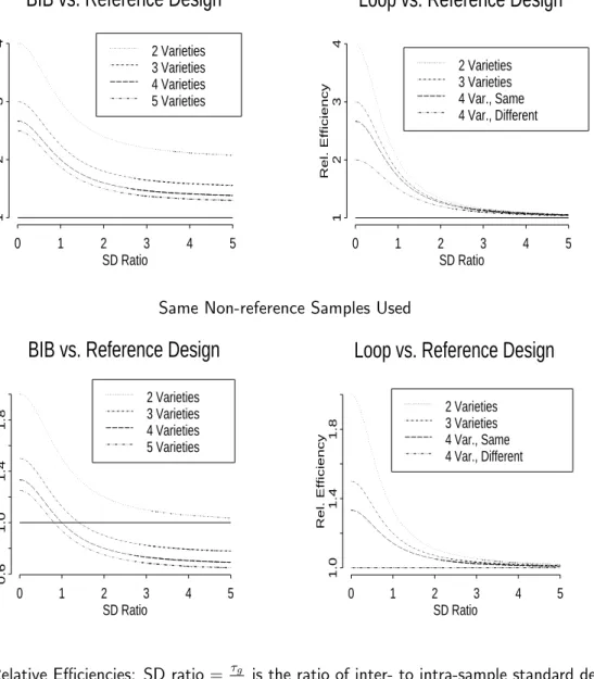
Analytic calculations show that the relative efficiencies of designs are functions of the ratio of inter- to intra-sample variation (for derivations, see supplementary material at
http://linus.nci.nih.gov/˜ brb/TechReport.htm). Analytic formulas are given in Tables 1 and 2. Results of these calculations are displayed in Figure 7. The top left plot in Figure 7 shows the results when the number of arrays is fixed for a BIB design with no subsampling. On the x-axis is the ratio of inter- to intra-sample standard deviation, i.e. τg
σg. On the y-axis is the relative
efficiency, that is, the ratio of the variance of effect contrasts in the reference design divided by the variance of the same contrasts in the balanced block design. For two varieties, the balanced complete block design performs better than the reference design because it utilizes twice as many non-reference specimens. The advantage of the block design degrades as inter-sample variance
τ2
g increases relative to the intra-sample variance σg2. As the number of varieties increases, the
advantage of the BIB design decreases.
The lower left plot in Figure 7 shows the results when the number of non-reference samples is fixed for a BIB design. No subsampling (of non-reference samples) is used for either the BIB or reference design. For two varieties, the relative efficiency of the block design converges quickly to
one, and the reference design performs better than the block design for more than two varieties when the inter-sample variance is large relative to the intra-sample variance.
Finally, we consider the loop design with two aliquots per sample. (This is the design that permits both cluster analysis and class comparison.) The BIB designs on the left side panels of Figure 7 do not permit cluster analysis, but the loop designs on the right side panels do. The upper right plot in Figure 7 shows the results when the number of arrays and non-reference specimens is fixed. The x-axis is again the ratio τg
σg, and the y-axis the corresponding relative efficiency. When
there are four or more varieties, the variance of contrasts depends on the positions of the varieties in the loop; “same” indicates varieties which appear together on the same array (e.g., varieties A and B in Figure 5) and “adjacent” indicates varieties which do not appear on the same array (e.g., varieties A and C in Figure 5). In this case, the relative efficiency quickly goes to one as the inter-sample variance increases relative to the intra-sample variance. The lower right plot in Figure 7 shows the results when the number of non-reference specimens is fixed and two aliquots of each non-reference specimen are used for each design. In this case, the relative efficiencies are reduced. This is under the assumption that one has access to a fixed number of samples and enough RNA to construct two subsamples from each, so that the reference design is forced to use the subsamples.
3.2 Clustering Performance Comparison of Designs
3.2.1 Mathematical Results
We consider clustering of samples (not genes). Cluster analysis algorithms take as input the distance between each pair of samples. In our ANOVA model, the differences in two samples are reflected in the sample by gene interaction, F Gf g. (The sample main effectsFf, if present, are assumed to be artifacts of the cDNA extraction process.) To simplify the investigation, we remove the variety effects from the model. This results in the normalization model
log(Yadf gr) = µ+Aa+Dd+ADad+Ff+²adf gr
where²adf gr are independent and normally distributed with mean zero and variance σ2. The gene
model is
radf gr = Gg+AGag+F Gf g+γadf gr
where γadf gr are independent and normally distributed with mean zero and variance σ2
g. Since
each pair of samples is to be compared, a BIB design will not generally be feasible, because forN
samples this would require at least N−1 aliquots of each sample. In this case, a loop design with
two aliquots per sample may be used, and is shown in Figure 6.
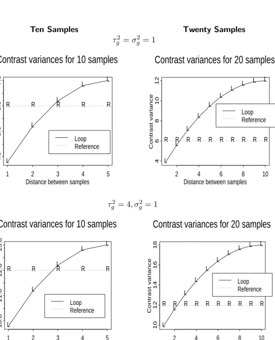
Theoretical calculations show that for the loop design, variance of contrasts will depend on how close together the samples appear in the loop. Figure 8 shows examples of the variance of contrasts
for samples of size 10 and 20, with τg =σg and with τg = 2σg. As the distance between samples
in the loop increases, these plots display the corresponding increase in the variance of contrasts. When there are 20 samples, the proportion of contrast estimates with greater variance under the loop design is larger than when there are 10 samples. Note that as the number of samples increases (beyond 20), this trend will continue. Hence, information about the distance between pairs of samples in a loop design will, on average, decrease as the number of samples increases. This suggests that the ability to correctly identify clusters under a loop design will break down as the number of samples increases.
3.2.2 Monte Carlo Cluster Performance Investigation
Cluster performance can best be evaluated by Monte Carlo simulation. We consider a case in which samples come from two groups, which differ in expression on a subset of genes. We consider two cases, one in which the inter-sample variance is equal to the intra-sample variance, i.e. τ2
g =σ2g,
and one in which the inter-sample variance is four times the intra-sample variance, i.e. τg2 = 4σg2. Data were simulated from one thousand genes, twenty of which were differentially expressed. The “spot” effect is simulated as a random effect with a normal distribution. The gene main effect is represented by a fixed effect. Parameter values for effect sizes were approximated using a subset of a prostate cancer microarray dataset. The base ten log of the intensity levels was the response. We generated data with gene main effect Gg = 2.5, and random spot effectAGag normal with mean
0 and variance 0.612; twenty genes were down-regulated in half the non-reference samples and
up-regulated in the other half; we looked at simulations where the distance between up-regulated and down-regulated genes was 2.5 and 1.8; for the rest of the 1,000 genes in the non-reference samples, and for all genes in the reference samples, gene effects were equal, so thatF Gf g = 0; we considered one scenario with inter-sample variance and intra-sample variance 0.432, and a second
with inter-sample variance.552 and intra-sample variance .272. For each Monte Carlo simulation,
one-half of the non-reference samples were selected at random to be down-regulated, and the rest were up-regulated.
For data simulated from the model we have described, the truth is that there are two clusters. In order to get a quantitative measure of performance, we specified that the algorithm should find two clusters. We used an hierarchical clustering algorithm with average linkage. Performance was measured by comparing a cluster to the best matching “true” group, then counting the number of discrepancies (omissions and additions) present.
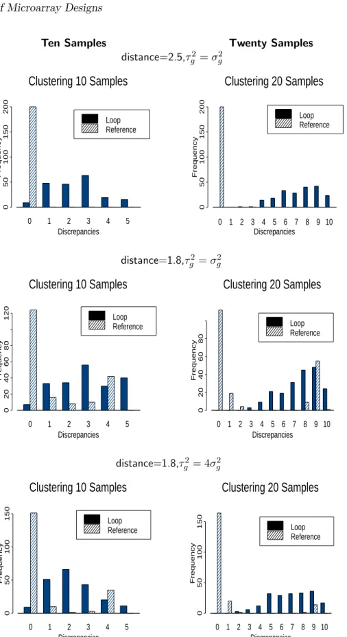
Simulation results appear in Figure 9. In the two top-most plots the distance between the means is 2.5 and the reference design does significantly better, having zero misclassifications on 98% of the simulations or more. The loop design does not appear to do well even for 10 samples, and as predicted by the analytic results, the relative performance of the loop design gets worse as the number of samples increases. The middle two plots show the effect of decreasing the distance between the true means in the simulation (from 2.5 to 1.8); in this case, the reference design still
performs better than the loop. One potential advantage of the loop design is that it uses two observations to estimate each sample effect as opposed to one for the reference design, and so may be less susceptible to outliers. The greater susceptibility to outliers of the reference design is apparent in the second mode in the distributions, reflecting cases in which a singleton was placed in one group. In the simulations discussed so far, we assumed that τg
σg = 1, i.e. inter-sample variance
equals intra-sample variance. These results were fairly stable over a range of values of τg
σg. As
τg
σg → 0, the loop design improves somewhat relative to the reference design. As
τg
σg → ∞, the
reference design improves relative to the loop design. An example is shown in the bottom two plots, which have parameter settings the same as the middle two plots except that now τg = 2σg.
4
Discussion
4.1 Summary
We have shown that comparison of microarray experimental designs is complicated by the presence of different levels of variability. Aliquots from a single RNA source are expected to be less variable than aliquots from different sources. As a result, the usual ANOVA assumption of equal error variance may not be satisfied. We have seen that this fact does not preclude a comparison of design efficiencies, although one will need some estimate of the approximate relation between inter-sample and intra-sample variance to get an explicit answer to the relative efficiency question.
We have also shown that cluster analysis results from a reference design can be much better than from a loop design, and that as the number of samples increases, the performance of cluster algorithms for the loop design gets worse. This is because information about the distances between samples is not the same for all samples in a loop design. The cluster analysis for a loop design should ideally weight the distances in the distance matrix to reflect the variability in the distance information. We did not pursue a weighted approach because our mathematical results indicate that the essential information problem would remain, and there is no methodology that is widely used for weighted cluster analysis.
4.2 Some Practical Robustness Issues
Here we discuss common issues that arise in microarray experiments which may impact design and analysis decisions, such as: low quality arrays, multiple possible taxonomies beforehand, arrays with multiple spots per gene, dye by gene interactions, array replication, use of blocking factors to reduce variability, and sample size calculation.
Damage to or inadequate quality of individual arrays can have a greater impact on cluster analysis in the loop design than the reference design. If two or more arrays are inadequate in a loop design, then the samples may be broken into non-communicating sets which would make cluster analysis impossible. If arrays are inadequate in a reference design, the ability to cluster the remaining samples will not be effected. Since quality control of RNA collection, array printing, and
hybridization can be significant problems, this is an important consideration.
It is common to have several potential taxonomies (or factors) at the design phase of an ex-periment. For example, one could group tumor samples based on tumor type, or on response to treatment, or on other histopathological features. One may not know ahead of time which tax-onomy will describe a meaningful difference in gene expression, and so will want to ensure the ability to make efficient comparisons between groups for each potential grouping of samples. If no reference sample is to be used, then allocating samples to arrays in a way that ensures all contrasts of interest can be estimated efficiently may be a significant design problem. The accuracy of the resulting estimates for some contrasts may also degrade if there are a small number of inadequate quality arrays. On the other hand, if a reference design is used, then the allocation of samples to arrays poses no design problem, and the resulting contrast estimates should be reasonably robust in the presence of a few low quality arrays.
If genes are spotted multiple times on each array, then variation in spots will no longer be captured by the array by gene interaction because several spots on a slide will share the same array and gene labels. Spot effects can then be captured by appending a spot location subscript to the array by gene interaction in the gene model (Equation 1), replacing AGag with AGLagl where l
indexes the location.
A concern in many microarray experiments is that some genes may incorporate a dye more or less efficiently than other genes (Kerr and Churchill, 2001; Tseng et al., 2001). Such effects would
be represented by a DG interaction term. In Section 2.1 we noted that for the reference design, variety contrast estimates are unbiased when aDGinteraction is present. For a BIB or loop design, failure to explicitly model theDGinteraction if one is present will generally result in biased variety contrast estimates unless the varieties are balanced with respect to the dyes, i.e. for every variety half the samples are tagged Cy3 and the other half Cy5. If several potential taxonomies (factors) are present, then designing the experiment so that each is balanced with respect to the dyes may be problematic. In addition, the common occurrence of low quality spots for a gene can destroy planned balance.
Although repeating arrays (i.e. having RNA from the same two sources on more than one array) will generally result in loss of efficiency, it may be desirable in some cases. For instance, some repeated arrays with reversed labelling allow one to estimate theDG interaction term; also, repeated arrays in a BIB design may allow one to estimate theF G interaction term and identify potentially problematic or influential samples.
Similarly, if some factors are not of interest, then one may wish to use these as blocks in a block design to gain efficiency. Creating blocks in a reference design is straightforward. Blocks may be formed in a loop design by creating a separate loop for each level of the blocking variable. Because each RNA sample will be associated with one level of the blocking variable, it will be associated with only one of these unconnected loops. One could not compare samples in different blocks. The loop design locks one into a blocked analysis where the reference design does not.
Correct sample size for a reference design can be calculated in a straightforward way using a log-ratio approach (Simon et al., 2002). With non-reference designs, established methods exist for calculating sample size and power curves for fixed effects and mixed effects models, and can be applied directly to array data (Wolfinger et al., 2001).
4.3 The Model Assumptions
Here we discuss some assumptions of the ANOVA modelling approach, and the impact violations would have on our results, including: inadequacies of the normalization model, correlation of resid-uals from the normalization model, and inadequacies of the gene model.
Some reviewers expressed concern that the normalization model may be inadequate for two reasons: it makes the unlikely assumption of equal error variance, and it performs the normalization in a linear fashion. We agree that the first assumption is unlikely if the effects in the gene-specific models are non-zero, but that assuming equal variance does produce least squares estimates of normalization model parameters, which we think reasonable. Some researchers believe that making a nonlinear adjustment to each array (Dudoit et al., 2000) is important because it corrects for dye bias associated with spot intensity. Our normalization model is really not essential to the results we have presented, and can be replaced by a different normalization procedure that corrects for the same effects before fitting the gene model. Our analytic and simulation results would still be valid, since they only rely on the structure of the gene model. Our main purpose here is to
compare experimental designs, and not necessarily solve the complex question of microarray data normalization.
We have modelled the residuals in the gene model as independent even though they are really correlated from the fitting of the normalization model. We do not think this is problematic. Note that the correlation of the residuals induced by fitting an ANOVA model is a function of the design matrix, and hence does not depend on effect size. Therefore, we can use matrix algebra to calculate the correlation created by fitting the normalization model for each pair of residuals, regardless of effect size. A computation shows that for any two residuals from the normalization model, the correlation induced by the model falls between−1
G and 0, where G is the number of genes. Since
the number of genes is large, the correlation will be practically zero. For instance, with 1000 genes, the correlation of every pair of residuals would fall between -.001 and 0; with 5000 genes, between -.0002 and 0. Such a minor violation of the independence assumption in the gene models is clearly of no practical concern. Also note that any array normalization methodology uses the data to perform the normalization, and will therefore induce correlation among the measured quantities at the gene level; as long as this correlation is very small, the benefits of normalization far outweigh the cost of creating an extremely small violation of independence. As the famous statistician George Box said some years ago, ”All models are wrong, but some are useful.” The success of microarray technology shows that these are useful models.
do not imply that the errors in the gene models will be correlated. For instance, if a collection of genes associated with proliferation have up-regulated expression levels in a subset of the samples, then this may cause the sample effect estimates,F Gd, in the different gene models to be correlated. But it will not induce correlation in the errors terms either within a particular gene model or in different gene models. Similarly, if a target gene hybridizes to two spots on an array, then estimated expression for the two genes associated with the spots may be correlated, but this again will not induce correlation in the error terms.
Our theoretical and Monte Carlo results rely on ANOVA assumptions and methods in the gene models in order to facilitate the comparisons between the different types of microarray designs. We believe the ANOVA approach to be reasonable, but if one uses this approach, the ANOVA assumptions need checking for specific data. Although ANOVA methods are fairly robust, if these assumptions appear to be seriously violated for a set of data, then this may be problematic for loop or block designs. If, for instance, the residuals for a particular gene appear to violate the assumption of normality, then the ANOVA results may be invalid. If a reference design was used, then more robust non-model based methods can be applied to the data. However, if a loop or block design was used, then the more complex relation between the groups over the arrays may make finding a robust alternative analysis technique difficult.
4.4 Size of the Inter-sample to Intra-sample Variance Ratio
The performance of the reference design, both in class discovery and class comparison, improves relative to the non-reference designs we have considered as the ratio of inter- to intra-sample variance increases. In order to evaluate a reasonable range of values for the ratio τg
σg, we analyzed data from
two breast cancer cell lines. The data consist of one mRNA sample from each cell line. Several arrays contained one aliquot from each sample, which allowed us to obtain explicit estimates of the ratio τg
σg for each of the 2,136 genes represented on the arrays. The normalization model had array
main effects, dye main effects, and array by dye interactions. Gene models with gene main effects, gene by array interactions, and with or without sample effects were fit to obtain estimates of τ2
g
and σ2
g. In this case, the variance between the cell lines reflects inter-sample variability, and the
variance within a cell line intra-sample variability. The median of the ratio estimates τˆg
ˆ
σg was 2.7;
73% of the ratios were above 1, indicating that inter-sample variability was larger than intra-sample variability, and 56% were above 2. These results indicate that in this experiment the ratio tended to be over 1 was over 2 for more than half the genes.
4.5 Conclusion
If class discovery is an objective of the experiment, then a reference design appears preferable to a loop design because of the potentially dramatic gain in cluster performance. If only class comparison is an objective of the experiment and there are sufficient samples available, then fairly
significant gains in efficiency are possible with a BIB design over a reference design, although these gains come with some loss of robustness to quality control problems. If, on the other hand, one has a limited number of samples available, then the reference design will probably be preferable, because it is likely to be more efficient than a BIB (or loop) design, while also being more robust.
REFERENCES
Alizadeh, A.A., Eisen, M.B., Davis, R.E., Ma, C., Lossos, I.S., Rosenwald, A., Boldrick, J.C., Sabet, H., Tran, T., Yu, X., Powell, J.I., Yang, L., Marti, G.E., Moore, T., Hudson Jr., J., Lu, L., Lewis, D.B., Tibshirani, R., Sherlock, G., Chan, W.C., Greiner, T.C., Weisenburger, D.D., Armitage, J.O., Warnke, R., Levy, R., Wilson, W., Grever, M.R., Byrd, J.C., Botstein, D., Brown, P.O., and Staudt, L.M. (2000) Distinct types of diffuse B-cell lymphoma identified by gene expression profiling. Nature,403, 503-511.
Ben-Dor, A., Bruhn, L., Friedman, N., Nachman, I., Schummer, M., and Yakhini, Z. (2000) Tissue Classification with Gene Expression Profiles. J. Comput. Biol.,7, 559-583.
Bittner, M., Meltzer, P., Chen, Y., Jiang, Y., Seftor, E., Hendrix, M., Radmacher, M., Simon, R., Yakhini, Z., Ben-Dor, A., Sampas, N., Dougherty, E., Wang, E., Marincola, F., Gooden, C., Lueders, J., Glatfelter, A., Pollock, P., Carpten, J., Gillanders, E., Leja, D., Dietrich, K., Beaudry, C., Berens, M., Alberts, D., Sondak, V., Hayward, N., and Trent, J. (2000) Molecular classification of cutaneous malignant melanoma by gene expression profiling. Nature,406, 536-540.
Brown, P.O. and Botstein, D. (1999) Exploring the new world of the genome with DNA microarrays.
Nat. Genet.,21, 33-37.
Cochran, W.G. and Cox, G.M. (1992) Experimental Designs, 2nd Ed. John Wiley & Sons, New York.
Dudoit, S., Yang, Y.H., Callow, M.J., and Speed, T.P. (2000) Statistical methods for identify-ing differentially expressed genes in replicated cDNA microarray experiments. Technical Report, http://www.stat.berkeley.edu/users/terry/zarray/TechReport/578.pdf.
Duggan, D.J., Bittner, M., Chen, Y., Meltzer, P. and Trent, J.M. (1999) Expression profiling using cDNA microarrays. Nat. Genet.,21, 10-14.
Eisen, M.B., Spellman, P.T., Brown, P.O., and Botstein, D. (1998) Cluster analysis and display of genome-wide expression patterns. Proc. Natl. Acad. Sci. U S A,95, 14863-14868.
Golub, T.R., Slonim, D.K., Tamayo, P., Huard, C., Gaasenbeek, M., Mesirov, J.P., Coller, H., Loh, M.L., Downing, J.R., Caligiuri, M.A., Bloomfield, C.D., and Lander, E.S. (1999) Molecular Classification of Cancer: Class Discovery and Class Prediction by Gene Expression Monitoring.
Science,286, 531-537.
Gruvberger, S., Ringn´er, M., Chen, Y., Panavally, S., Saal, L.H., Borg, ˚A., Fern¨o, Peterson, C., and Meltzer, P.S. (2001) Estrogen Receptor Status in Breast Cancer Is Associated with Remarkably Distinct Gene Expression Patterns. Cancer Res.,61, 5979-5984.
Hastie, T., Tibshirani, R., Eisen, M.B., Alizadeh, A., Levy, R., Staudt, L., Chan, W.C., Botstein, D. and Brown, P. (2000)‘Gene shaving’ as a method for identifying distinct sets of genes with similar expression patterns. GenomeBiology.com1(2),
research0003.1-0003.21.
Hedenfalk, I., Duggan, D., Chen, Y., Radmacher, M., Bittner, M., Simon, R., Meltzer, P., Guster-son, B., Esteller, M., Raffeld, M., Yakhini, Z., Ben-Dor, A., Dougherty, E., Kononen, J., Bubendorf, L., Fehrle, W., Pittaluga, S., Gruvberger, S., Loman, N., Johannsson, O., Olsson, H., Wilfond, B., Sauter, G., Kallioniemi, O., Borg, ˚A, and Trent, J. (2001) Gene-expression Profiles in Hereditary Breast Cancer. N. Engl. J. Med.,344, 539-548.
Kerr, M.K. and Churchill, G.A. (2001) Experimental design for gene expression microarrays. Bio-statistics,2, 183-201.
Lee, M.L.T., Kuo, F.C. Whitmore, G.A., and Sklar, J. (2000) Importance of replication in microar-ray gene expression studies: Statistical methods and evidence from repetitive cDNA hybridizations.
Proc. Natl. Acad. Sci. U S A,97, 9834-9839.
McShane, L.M., Radmacher, M.D., Freidlin, B., Yu, R., Li, M. and Simon, R. (2001) Methods for assessing reproducibility of clustering patterns observed in analyses of microarray data. Technical Report, http://linus.nci.nih.gov/brb/TechReport.htm.
Radmacher, M.D., McShane, L.M., and Simon, R. (2001) A Paradigm for Class Prediction Using Gene Expression Profiles. Technical Report,
http://linus.nci.nih.gov/brb/TechReport.htm.
Scheff´e, H. (1999)The Analysis of Variance. John Wiley & Sons, New York.
Simon, R., Radmacher, M.D., and Dobbin, K. (2002) Design of Studies Using DNA Microarrays.
Genetic Epidemiology, in press.
Sudarsanam, P., Iyer, V.R., Brown, P.O., and Winston, F. (2000) Whole-genome expression analysis of snf/swi mutants of Saccharomyces cerevisiae. Proc. Natl. Acad. Sci. U S A,97, 3364-3369.
Tanaka, T.S., Jaradat, S.A., Lim, M.K., Kargul, G.J., Wang, X., Grahovac, M.J., Pantano, S., Sano, Y., Piao, Y., Nagaraja, R., Doi, H., Wood III, W.H., Becker, K.G., and Ko, M.S.H. (2000) Genome-wide expression profiling of mid-gestation placenta and embryo using a 15,000 mouse developmental cDNA microarray. Proc Natl Acad Sci U S A,97, 9127-9132.
Tseng, G.C., Oh, M.K., Rohlin, L., Liao, J.C., and Wong, W.H. (2001) Issues in cDNA microarray analysis: quality filtering, channel normalization, models of variations and assessment of gene effects. Nucleic Acids Research,29, 2549-2557.
Wolfinger, R.D., Gibson, G., Wolfinger, E.D., Bennett, L., Hamadeh, H., Bushel, P., Afshari, C., and Paules, R.S. (2001) Assessing Gene Significance from cDNA Microarray Expression Data via Mixed Models. J. Comput. Biol., in press
A
Figure Legends
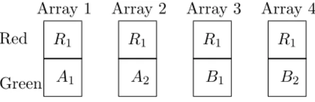
Figure 1: Reference Design Example: Two samples from each of two varieties of interest. One aliquot from each non-reference sample. R1 represents a subsample from the reference sample. Aa
represents sampleafrom varietyA. Bb represents samplebfrom varietyB. Single replicate shown.
Figure 2: Loop Design Example: Two samples from each of two varieties. One aliquot from each sample. Single replicate shown.
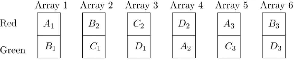
Figure 3: Loop Design Example: Two samples from two varieties or phenotypes. Two aliquots from each sample. Design allows for both cluster and ANOVA analysis.
aliquot from each sample. A single replicate is shown.
Figure 5: Loop Design Example: Two samples from each of four varieties or phenotypes. One aliquot from each sample.
Figure 6: Loop Design for Cluster Analysis: Two aliquots from each ofN samples. Ssrepresents an aliquot from samples.
Figure 7: Relative Efficiencies: Top Left: Reference Design vs. BIB Design; x-axis is ratio
τg
σg. y-axis is
varref(V Gc1g−V Gc2g)
varbb(V Gc1g−V Gc2g)
where varref indicates variance under a reference design, and varbb
variance under a balanced block design. Same number of arrays used on each design. One aliquot from each sample case. Bottom Left: Same as above but with equal total number of non-reference samples used on each design. Top Right: Reference Design Versus Loop Design; two aliquots per sample in loop design; x-axis is ratio τg
σg. y-axis is
varref(V Gc1g−V Gc2g)
varloop(V Gc2g−V Gc1g)
wherevarloopindicates variance
under a loop design. Same number of arrays used on each design. For 4 varieties case, “Same” indicates varieties appear together on the same array in the loop design, and “adjacent” indicates that they do not. Bottom Right: Same as above but with the same set of non-reference subsamples used on each design.
Figure 8: Contrast variance of simple reference design and loop design. Distance = 1 + (number of samples between the two samples of interest in the loop, taking shortest route).
of which are differentially expressed in two true sample clusters. Parameter values used to simulate data were approximated from cancer data. Bar height represents Monte Carlo simulations (out of 200) with corresponding number of discrepancies. Topmost plots: Inter-sample variance is equal to intra-sample variance. Distance between the differentially expressed genes is 2.5. Middle plots:
Same with distance reduced to 1.8. Bottommost Plots: Inter-sample standard deviation twice intra-sample standard deviation. Distance is 1.8.
B
Figures
Array 1 A1 R1 Array 2 A2 R1 Array 3 B1 R1 Array 4 B2 R1 Red GreenFigure 1: Reference Design Example Array 1 B1 A1 -Array 2 B2 A2 $ % Red Green ' &
-Figure 2: Loop Design Example Array 1 B1 A1 Array 2 A2 B1 Array 3 B2 A2 Array 4 A1 B2 Red Green - - - $ % ' &
Array 1 B1 A1 Array 2 C1 B2 Array 3 D1 C2 Array 4 A2 D2 Array 5 C3 A3 Array 6 D3 B3 Red Green
Figure 4: Balanced Incomplete Block Example
Array 1 B1 A1 Array 2 C1 B2 Array 3 D1 C2 Array 4 A2 D2 Red Green - - - $ % ' &
-Figure 5: Loop Design Example
Array 1 S2 S1 Array 2 S3 S2 ... Array N S1 SN Red Green - - - $ % ' &
No Subsampling Loop with Two Subsamples/Sample Same Number of Arrays Used
BIB vs. Reference Design
SD Ratio Rel. Efficiency 1 2 3 4 0 1 2 3 4 5 2 Varieties 3 Varieties 4 Varieties 5 Varieties
Loop vs. Reference Design
SD Ratio Rel. Efficiency 1 2 3 4 0 1 2 3 4 5 2 Varieties 3 Varieties 4 Var., Same 4 Var., Different
Same Non-reference Samples Used
BIB vs. Reference Design
SD Ratio Rel. Efficiency 0.6 1.0 1.4 1.8 0 1 2 3 4 5 2 Varieties 3 Varieties 4 Varieties 5 Varieties
Loop vs. Reference Design
SD Ratio Rel. Efficiency 1.0 1.4 1.8 0 1 2 3 4 5 2 Varieties 3 Varieties 4 Var., Same 4 Var., Different
Figure 7: Relative Efficiencies: SD ratio= τg
σg is the ratio of inter- to intra-sample standard deviation.
Rel. Efficiency = varref(V Gc1g−V Gc2g)
varalt(V Gc1g−V Gc2g)
where varref indicates variance under a reference design, and
Ten Samples Twenty Samples τ2
g =σ2g = 1
Contrast variances for 10 samples
Distance between samples
Contrast variance 1 2 3 4 5 4.0 5.0 6.0 7.0 R R R R R L L L L L Loop Reference
Contrast variances for 20 samples
Distance between samples
Contrast variance 2 4 6 8 10 4 6 8 10 12 R R R R R R R R R R L L L L L L L L L L Loop Reference τ2 g = 4, σg2= 1
Contrast variances for 10 samples
Distance between samples
Contrast variance 1 2 3 4 5 10.0 11.0 12.0 13.0 R R R R R L L L L L Loop Reference
Contrast variances for 20 samples
Distance between samples
Contrast variance 2 4 6 8 10 10 12 14 16 18 R R R R R R R R R R L L L L L L L L L L Loop Reference
Ten Samples Twenty Samples distance=2.5,τ2 g =σ2g 0 50 100 150 200
Clustering 10 Samples
Discrepancies Frequency 0 1 2 3 4 5 Loop Reference 0 50 100 150 200Clustering 20 Samples
Discrepancies Frequency 0 1 2 3 4 5 6 7 8 9 10 Loop Reference distance=1.8,τ2 g =σ2g 0 20 40 60 80 120Clustering 10 Samples
Discrepancies Frequency 0 1 2 3 4 5 Loop Reference 0 20 40 60 80Clustering 20 Samples
Discrepancies Frequency 0 1 2 3 4 5 6 7 8 9 10 Loop Reference distance=1.8,τ2 g = 4σg2 0 50 100 150Clustering 10 Samples
Discrepancies Frequency 0 1 2 3 4 5 Loop Reference 0 50 100 150Clustering 20 Samples
Discrepancies Frequency 0 1 2 3 4 5 6 7 8 9 10 Loop ReferenceC
Tables
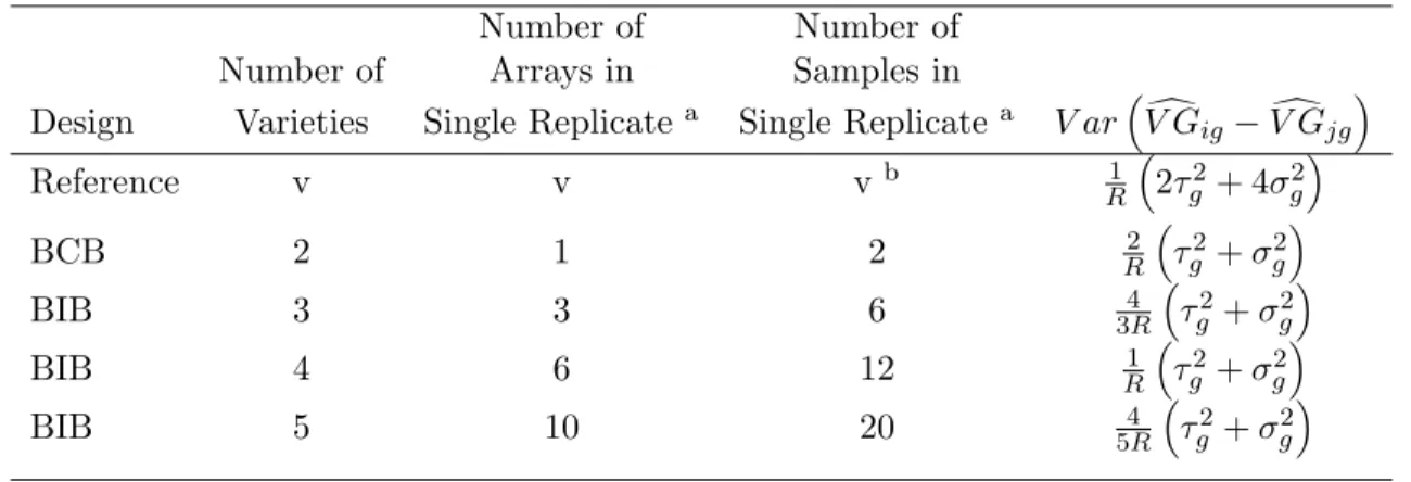
Contrast Variances: No Subsampling Number of Number of Number of Arrays in Samples in
Design Varieties Single Replicatea Single Replicatea V ar³V Gdig−V Gdjg´
Reference v v vb 1 R ³ 2τ2 g + 4σ2g ´ BCB 2 1 2 R2 ³τg2+σ2g´ BIB 3 3 6 4 3R ³ τ2 g +σ2g ´ BIB 4 6 12 1 R ³ τ2 g +σ2g ´ BIB 5 10 20 4 5R ³ τ2 g +σ2g ´
Table 1: Variances of contrasts for reference, balanced complete block (BCB), and balanced incomplete block (BIB) designs. One aliquot from each non-reference sample used. Contrast variances are the same for all pairs of (non-reference) samples i and j. In the first row, v is the number of varieties, and the contrast variance formula is the same for all v. For the block designs, the contrast variance formula varies depending on the number of varieties. R is the number of replicates.
aA single replicate for a reference design is a collection of microarrays arranged so that every array contains
one sample from a variety of interest paired with one aliquot from the reference sample, and there are enough arrays so that one sample from each variety of interest is present. A single replicate for a balanced block design is a collection of microarrays arranged so that every array contains two samples, each from a different variety, and there are enough arrays so that every variety appears exactly once on an array with every other variety. (For detailed diagrams of designs, see Supplementary Material at http://linus.nci.nih.gov/ brb/TechReport.htm.)
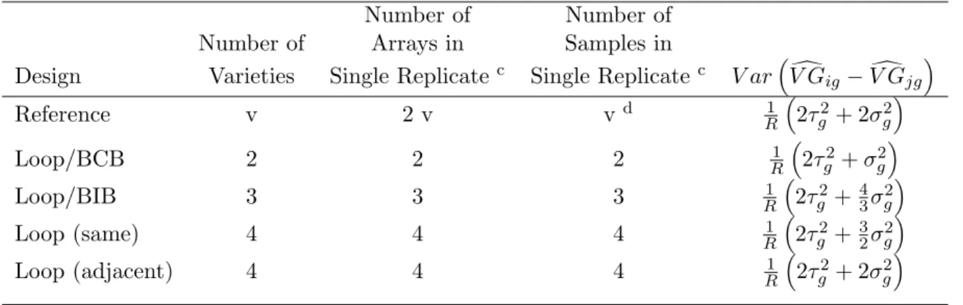
Contrast Variances: Two Aliquots Per Sample Number of Number of
Number of Arrays in Samples in
Design Varieties Single Replicatec Single Replicatec V ar³V Gdig−V Gdjg´
Reference v 2 v vd R1 ³2τg2+ 2σg2´ Loop/BCB 2 2 2 R1 ³2τg2+σg2´ Loop/BIB 3 3 3 R1 ³2τg2+43σg2´ Loop (same) 4 4 4 1 R ³ 2τ2 g +32σg2 ´ Loop (adjacent) 4 4 4 1 R ³ 2τ2 g + 2σg2 ´
Table 2: Variances of contrasts for reference and loop designs. Two aliquots from each non-reference sample used. In the first row, v is the number of varieties, and the contrast variance formula is the same for all v, although the number of arrays required varies. For the loop designs, the the number of arrays required and the contrast variance vary depending on the number of varieties. For 4 or more arrays, the variance of contrasts also depends on the relative positions of the varieties in the loop; “same” indicates varieties which appear together on an array, and “adjacent” varieties which do not.
R is the number of replicates.
cA single replicate for reference design is a collection of microarrays arranged so that every array contains one sample
from a variety of interest paired with one aliquot from the reference sample, and there are enough arrays so that one sample from each variety and two aliquots from each sample are represented. A single replicate for a loop design is a collection of microarrays arranged so that every array contains two aliquots, each from a different sample, there are enough arrays so that two aliquots from each sample are represented, and the samples are arranged in a loop design (see Figure 6).