CFIRE December 2009

MODEL FOR SHIPPING

COMMODITIES BY TRUCK

CFIRE 02-30

December 2009

National Center for Freight & Infrastructure Research & Education

College of Engineering

Department of Civil and Environmental Engineering

University of Wisconsin, Madison

Authors:

Mazen I. Hussein and Matthew E. H. Petering

Center for Urban Transportation Studies University of Wisconsin – Milwaukee

Principal Investigator:

Alan J. Horowitz

Professor, Civil Engineering and Mechanics Department, University of Wisconsin – Milwaukee

1. Report No.

CFIRE 02-30

2. Government Accession No. 3. Recipient’s Catalog No.

CFDA 20.701

4. Title and Subtitle

A POLICY-ORIENTED COST MODEL FOR SHIPPING COMMODITIES BY TRUCK

5. Report Date December 2009 6. Performing Organization Code 7. Author/s

Mazen I. Hussein and Matthew E. H. Petering, University of Wisconsin-Milwaukee

8. Performing Organization Report No.

CFIRE 02-30

9. Performing Organization Name and Address

National Center for Freight and Infrastructure Research and Education (CFIRE) University of Wisconsin-Madison

1415 Engineering Drive, 2205 EH Madison, WI 53706

10. Work Unit No. (TRAIS) 11. Contract or Grant No.

DTRT06-G-0020

12. Sponsoring Organization Name and Address

Research and Innovative Technology Administration U.S. Department of Transportation

1200 New Jersey Ave, SE Washington, D.C. 20590

13. Type of Report and Period Covered

Final Report 10/1/07 – 9/30/09]

14. SponsoringAgency Code 15. Supplementary Notes

Project completed for USDOT’s RITA by CFIRE.

16. Abstract

Surprisingly, transportation planners and policy makers do not have the ability to estimate the cost of shipping a quantity of a commodity between two locations for broad categories of goods. Costs of shipping are important components in mode, route, and location choice processes. Good knowledge of costs can aid public sector decision makers in determining the economic benefits of infrastructure improvements or determining the impacts on the private sector of various policies and operational strategies. Shipping costs relate to logistics practices of businesses, and these practices have been changing rapidly in recent years. In this study, we inventory cost models that have been used in the past and evaluate the availability of data sets containing shipment cost information. We then build a cost model for shipping various commodities and commodity groups by truck and present several examples to show how the model can address issues of interest to carriers, shippers, and governments.

17. Key Words

Commodities, shipping, cost, freight

18. Distribution Statement

No restrictions. This report is available through the Transportation Research Information Services of the National Transportation Library.

19. Security Classification (of this report)

Unclassified

20. Security Classification (of this page)

Unclassified

21. No. OfPages 61

22. Price

-0-

This research was funded by the National Center for Freight and Infrastructure Research and Education. The contents of this report reflect the views of the authors, who are responsible for the facts and the accuracy of the information presented herein. This document is disseminated under the sponsorship of the Department of Transportation, University Transportation Centers Program, in the interest of information exchange. The U.S. Government assumes no liability for the contents or use thereof. The contents do not necessarily reflect the official views of the National Center for Freight and

Infrastructure Research and Education, the University of Wisconsin, the Wisconsin Department of Transportation, or the USDOT’s RITA at the time of publication. The United States Government assumes no liability for its contents or use thereof. This report does not constitute a standard, specification, or regulation.

The United States Government does not endorse products or manufacturers. Trade and manufacturers names appear in this report only because they are considered essential to the object of the document.

2

A Policy-Oriented Cost Model for Shipping Commodities by Truck

Abstract: Surprisingly, transportation planners and policy makers do not have the ability to estimate the cost of shipping a quantity of a commodity between two locations for broad categories of goods. Costs of shipping are important components in mode, route, and location choice processes. Good knowledge of costs can aid public sector decision makers in determining the economic benefits of infrastructure improvements or determining the impacts on the private sector of various policies and operational strategies. Shipping costs relate to logistics practices of businesses, and these practices have been changing rapidly in recent years. In this study, we inventory cost models that have been used in the past and evaluate the availability of data sets containing shipment cost information. We then build a cost model for shipping various commodities and commodity groups by truck and present several examples to show how the model can address issues of interest to carriers, shippers, and governments.

INTRODUCTION

Freight can be broadly defined as the movement of goods from one place to another. The United States freight transportation network consists of hundreds of thousands of miles of

transportation infrastructure and hundreds of thousands of transportation facilities devoted to five different modes of transport: road, rail, air, water, and pipeline. Increases in population,

economic activity, and global trade have put tremendous pressure on this network in recent years. Indeed, it appears that the U.S. is now reaching a crossroads with respect to transportation planning that calls for drastic action. With the majority of transportation infrastructure in the public domain, the best chance for change lies with federal, state, and local policy makers. During the next few years, it is crucial for elected and non-elected public officials to adopt wise policies that will chart a favorable course for the U.S. transportation system in the 21st century.

Transportation policies are usually judged in terms of their environmental, social, and economic impacts. Economic impact usually dominates policy analysis, with environmental and social impacts playing a secondary role. Yet, even economic analysis of transportation policy is often incomplete. In particular, the impact of a proposed project or policy on private sector shipping costs is rarely studied. Instead, most analyses focus on the jobs created by an infrastructure project; the public sector infrastructure and maintenance costs of the project or policy; and the impact on traffic congestion. Meanwhile, the discussion of costs borne by private sector shipping companies is muted. The purpose of the current study is to develop a

methodology that will allow private sector shipping costs to become a larger part of the equation in transportation policy analysis.

Freight transportation costs are of interest to at least three kinds of institutions—carriers, shippers, and governments. Carriers need to know freight transportation costs because they are the providers of transportation services. Shippers need to have a handle on freight transportation costs in order to better understand decisions regarding facility location and supply chain

management. Finally, governments need to be able to estimate freight transportation costs if they are to formulate sound transportation policies. Surprisingly, these costs have played only a minor role in transportation planning and policy analysis. Shipping costs are an important

3 component of mode, route, and location choice decision making processes in the freight industry. Good knowledge of shipping costs is therefore vital to the formulation of effective public policy. For example, it is important for policy makers to know how potential changes in truck flows, sizes, and weights could affect shipping costs. It is also important for transportation officials to know how proposed infrastructure improvements or construction projects affect shipping costs for different economic sectors.

In order to raise the profile of private sector shipping costs in freight transportation policy analysis, there needs to be a method for estimating the cost of shipping commodities between any two locations. At the moment, there are a few tools developed by academic researchers that can estimate the cost of shipping individual commodities between any two locations. However, to the authors’ knowledge, no tools are designed to estimate the costs of shipping broad

categories of cargo that correspond to various sectors of the U.S. economy. Thus, a policy-oriented methodology for estimating shipping costs is still missing.

In this study, we inventory freight cost models that have been used in the past and evaluate the availability of data sets containing shipment cost information. We then develop a methodology for estimating shipping costs for one freight transportation mode—trucking. U.S. Census figures indicate that shipments by truck were valued at about USD $6235 billion in 2002. This represents 75% of the total value of all shipments made within the U.S. The main objective is to build a model that can estimate the cost of shipping a certain quantity of a specific

commodity or commodity group by truck from any origin to any destination inside the United States. The model can also be used to estimate general shipping costs for different economic sectors, with significant ramifications for public policy. The field-testing of the model and expansion of the model to include at least one additional mode of transportation—rail, air, or water—is left to a future study.

This paper is organized as follows. Section 2 reviews the literature relevant to the current study. In Section 3, we evaluate the availability of data sets containing shipment cost

information. Section 4 introduces the concept of commodity aggregation as a way to model shipping costs from a public policy perspective. A mathematical model of shipping costs in the trucking industry is presented in Section 5. In Section 6, we illustrate the use of the cost model in various hypothetical scenarios. Final conclusions are made in Section 7.

LITERATURE REVIEW

A literature review was conducted to determine what research has already been done on freight planning and other topics related to freight cost modeling.

Berwick and Dooley (1997) built a truck cost model for motor vehicle owners and/or operators. A spreadsheet simulation model was developed to estimate truck costs for different truck configurations, trailer types, and trip movements. A shipper may need to know product unit costs to determine the transportation cost per item. Alternatively, a lessor (shipper) may want total trip costs while the owner/operator may want per hour or per mile costs. The trucking industry has a perfect competition environment due to its non-homogeneity, limited entry

barriers, large number of firms, and virtually perfect information. Furthermore, its small independent truckers are mainly price takers. Therefore, cost tracking and control are essential for survival of the owner/operator. However, the authors point out that owner/operators may have less knowledge of the full cost of their operation than shippers, larger trucking companies,

4 and logistics firms. Cost information is important because it allows shippers to reconcile freight rates with trucking costs. This may assure revenue adequacy for the truckers, without sacrificing efficiency in the shippers' industry. Current cost estimates may be beneficial to both parties (lessor and trucker) in negotiating a lease agreement. Sustainability for the independent trucker may reduce search costs, improve quality for the lessor, and reduce turnover.

Recent changes in manufacturing practice and supply chain management have lowered inventories and created a move toward just-in-time inventory management. These new changes have increased the need for quality transportation. With owner/operators moving 30 to 40 percent of all intercity freight (Griffin and Rodriguez, 1992), the importance of understanding the costs borne by owner/operators cannot be understated. The model proposed by Berwick and Dooley (1997) was the first effort to understand such costs.

Berwick and Dooley point out that change in trailers and combinations of trailers continue to affect the cost structure of the trucking industry. New safety requirements have affected the costs for truckers. Safety costs such as anti-lock braking systems and air ride suspension have added to the price of a new tractor and trailer. However, safety features may reduce risk (insurance) costs because of fewer crashes and less damage to products hauled. The use of cell phones and other technological changes also may create more changes in the trucking industry. The authors develop a spreadsheet model that contains several sheets. One of them contains decisions and exogenous variables, another one has performance measures, and the remaining sheets contain data and sensitivity analysis calculations, and linkages for the costing and revenue associated with particular truck movement. Fixed costs in this model include equipment costs, depreciation, return on investment, license fees insurance and sales tax, and management and overhead costs, while the variable costs include labor, fuel, tires, and maintenance and repair costs.

Berwick and Farooq (2003) continue the work of Berwick and Dooley. They argue that, while the spreadsheet costing model developed in 1996 was useful, it lacked the functionality of a stand-alone model or software product. Thus, a new visual basic model was developed to be a stand-alone product to be utilized by transportation professionals and researchers.

William and Allen (1996) find that the cost per mile of operating a motor vehicle is a key parameter in many transportation studies. They defined the auto operating cost as a result of dividing the sum of annual cost of maintenance, oil, and tires by average miles driven vehicle per year.

Forkenbrock (1999) defines private costs as the direct expenses incurred by providers of fright transportation. Such costs consist of operating costs, as well as investments in capital facilities while the external costs include: accident; emissions; noise; and unrecovered costs associated with the provision, operation, and maintenance of public facilities. Freight trucking creates certain adverse impacts. These impacts are referred to as external costs because they are not borne by those who generate these costs. Internalizing external costs makes it possible to return to society an amount equal to the costs one imposes. Forkenbrock’s analysis reveals that external costs are equal to 13.2% of private costs and user fees would need to be increased about three fold to internalize these external costs. These results depend on the data of intercity truck freight transportation which accounts for a very large share of the total ton-miles of

5 Forkenbrock (2001) extends the above work related to external costs of intercity truck freight transportation to include rail transportation and makes a comparison between the trucking and rail transportation modes. He finds that rail external costs are USD $0.24 to $0.25 per ton-mile, well less than the $1.11 for freight trucking, but that external costs for rail generally

constitute a larger amount relative to private costs—9.3% to 22.6%--than is the case for trucking (13.2%).

Ergun et al. (2007) propose an optimization model for reducing truckload transportation costs. A highly effective and extremely efficient heuristic had been designed and implemented that incorporates fast routines for checking time feasibility for a tour in the presence of dispatch time windows and for minimizing the duration of a tour by appropriately selecting a starting location and departure time.

Woensel and Curz (2009) studied the costs of transportation congestion. They show that contemporary traffic pricing typically does not reflect the external congestion costs. In order to induce road users to make the correct decision, marginal external costs should be internalized. Optimal use of a transportation facility cannot be achieved unless each additional user pays for the additional costs that he/she imposes on all other users on the facility. The main advantage of the authors’ methodology is the possibility to derive the marginal congestion costs in an

analytical way while taking into account the inherent stochasticity of the real world. This approach relies less on the availability of data than most other techniques.

One of the most comprehensive freight studies that has been done is described in Report 260 of the National Cooperative Highway Research Program (NCHRP 260). NCHRP is

administered by the Transportation Research Board (TRB) and sponsored by various state DOTs in cooperation with the Federal Highway Administration (FHWA). NCHRP was created in 1962 as a means to conduct research in acute problem areas that affect highway planning, design, construction, operation, and maintenance nationwide. NCHRP Report 260 proposes and describes a set of freight demand forecasting techniques that together form a ―user’s manual.‖ This user’s manual is a guide for conducting studies that involve or require freight demand forecasts. Its development is motivated by the observation that freight oriented studies are often adversely affected by inadequate freight flow data. Indeed, in most states the collection of truck traffic flow data, and the preparation of demand forecasts is treated as an appendage to similar data collection and forecasting that is done for passenger vehicles. Thus, passenger flows have received the majority of attention, while freight flows have been largely ignored.

The limited capability for undertaking truck-oriented freight demand forecasts in both highway and non-highway modes stems more from the lack of a database rather than from any inability to devise suitable truck traffic forecasting techniques. The lack of freight flow data usually means that future truck volumes are forecasted as a percentage of aggregated traffic volumes for both existing and proposed facilities. Thus, forecasts are usually prepared using trend extension forecasting techniques rather than by relating observed volumes with present economic activities. NCHRP proposes a method that can still accomplish freight demand forecasting despite the limited freight flow data. The NCHRP user’s manual presents an overall process or methodology to be followed in conducting such studies along with appropriate sub-techniques. Before attempting to apply the technique the user should first take time to fully determine the parameters and constraints both affecting and shaping the application at hand. Secondly, the user should reduce the scope of application to the maximum extent possible.

6 The overall freight demand forecasting technique consists of four phases: (1) traffic generation; (2) traffic distribution; (3) mode division; and (4) traffic assignment. The product of freight traffic generation and distribution is one or more commodity flow matrices. These

matrices show how much of a given commodity is being shipped between any two locations. A multidimensional commodity flow matrix may differentiate cargo according to commodity class, mode, shipment origin, and shipment destination and can be reported in annual tons, annual dollar value, and annual ton-miles. One matrix represents the base case. The others, developed from the base case matrix, represent predictions for future years. If vehicular origin-destination or commodity flow data are available to the user, that data should be used as the basis of the base year commodity flow matrix. The need for additional matrices depends on the alternatives being evaluated, the extent to which the application involves alternative (1) futures (cases of increasing or decreasing commodity or vehicle flow); (2) scenarios (changes in infrastructure, rates, or services); and/or (3) conditions (when constraints or limitations are placed upon system use or revenue and cost structure).Phase 3—mode division—consists of three main components: (1) summarizing base commodity (or vehicle) flows, carrier costs, and carrier revenue/shipper costs; (2) for each alternative being considered, dividing commodity flow among competing modes using a split model, and then summarizing resulting flows, costs, and revenues; and (3)

performing selected constancy tests to insure the reasonableness of the results obtained from the mode split model, and then preparing final outputs. Phase 4—traffic assignment—consists of four main components: (1) converting commodity flows into vehicle flows, if not already done in estimating carrier costs; (2) assigning the resulting traffic to modal networks; (3) estimating changes in vehicle/vessel volumes and loadings expected to occur on a segment basis; and (4) for highway segments, estimating expected changes in pavement service life on a segment basis.

The NCHRP 260 user’s manual contains three sub-techniques related to the freight cost. These are (1) a truck unit costing model, (2) a shipper costing model, and (3) a freight rate

estimating model. The truck unit cost sub-technique estimates the per-mile cost contributions for 16 components including insurance, fuel, and driver wages. These components are then

combined to produce estimates for the truck load cost, cost per mile, and cost per ton-mile. The model has a total of 35 variables. Users must provide eight specific inputs including fuel price ($/gallon) and can interactively change any of the remaining 27 variables or use supplied default values. As unit cost varies with the carrier, mode, and time, the resulting cost estimate is very rough and is not intended to be a true cost. Indeed, today most large carriers have developed extensive costing systems for strategic planning and internal management purposes.The second cost model is a shipper costing model. In recent years, shippers have increasingly recognized that the mode offering the lowest rate may not in fact be the least cost mode, after considering other logistics costs. Thus, costs accruing to shippers typically include transport logistics (rates, loss and damage, pickup and delivery) and non-transport logistics costs (order, storage,

inventory, and stock-out costs). These costs are taken into account in the shipper cost model. The third model is a rate estimating model. Completely separate from unit costs are the rates charged for specific transport services. Rates may be supplemented by charges for special or accessorial services and penalties assessed. Rates, charges, and penalties, taken together, represent carrier income. None of the above costing models directly consider issues related to public policy.

Huang and Smith (1999) mention that many state departments of transportation are becoming interested in developing statewide truck travel-demand (TTD) forecasting models. Estimates of future truck traffic are useful for making better decisions on highway

7 improvements. Four similar TTD models are developed for Wisconsin using 1993 Commodity Flow Survey (CFS) origin-destination (O-D) data and a limited amount of truck classification count data. First, statewide zonal-level trip tables are developed from the CFS database. Then, gravity models for four trip types are calibrated to match the trip-length frequency distributions of the CFS O-D trip tables. Finally, zonal trip productions and attractions are adjusted using an iterative procedure. The four alternative TTD models differ only in the method used to assign external trips to the external stations. All of the models provide reasonable levels of goodness-of-fit to the 40 selected calibration links, as well as 104 additional count locations across the state.

Gordon and Pan (2001) propose a three step modeling structure for the non-survey freight transportation model which includes freight trip generation, freight trip distribution and freight traffic assignment. A freight origin-destination (OD) matrix of freight flows can be developed using secondary data sources. The estimated freight flows can be loaded together conventional passenger flows on the regional high way network of a large metropolitan area. GIS can potentially improve the non-survey approach in data validation, model operations, and evaluation.

Tadi and Balbach (1994) mention that trip generation rates for trucks are lower than rates for autos in the case of all land use categories except for truck terminals. This appears logical as the main activity at truck terminals relates to trucks.

García-Ródenas and Marín (2009) established a new methodology to model and to simultaneously solve the problems of calibration and O-D (origin-destination) matrix estimation for the multi-modal assignment problem with combined modes (MAPCM). A new approach called the calibration and demand adjusting model (CDAM), has been formulated based on nonlinear bi-level programming. The existence of an infinite number of solutions for any reasonable means of calibration of the MAPCM is proved. This is due to the use of a nested logit model for the modeling of the demand and the cost structure of the model. A heuristic column generation algorithm (HCGA) has been proposed to solve the bi-level model.

De Jong, Gunn, and Walker (2004) found that national model systems that can be used for forecasting future freight transport volumes and/or vehicle flows have been developed in a number of European countries. For the trip generation step, several European and national models now use input-output and related methods. Distribution in those models is also based on input-output analysis, or in gravity formulations. For modal split, many different model forms can be found in practice. But most of the large model systems use multi-modal network assignment, in which mode choice and assignment are handled simultaneously.

Internationally, the Great Britain Freight Model (GBFM) is perhaps the most comprehensive freight demand forecasting model to be developed outside the United States (GBFM, 2003). The GBFM project objective was to combine a group of existing software components and data sources into a single entity, and to develop a comprehensive model of international and domestic freight flows within Great Britain.GBFM used a path enumeration technique which is the process of defining sequences of links connecting the source (origin) to the sink (destination). By attaching the trip matrix to a route choice model, traffic can be

assigned back to the underlying network, so that the assigned traffic volumes for a given link can be recorded. A basic concept of a network path freight network used in this model can be

simplified to that ofa ―service.‖ A service can be regarded as a wrapper for a path, where only thecustomer-oriented information (cost, time taken, reliability, access terminal, egressterminal)

8 are known. Within GBFM, it is possible to define services that can be added directly to the paths within the choice set, or as hyper-links within the multimodal network. In principle, this choice model, expressed as a mapping from generalized cost i to probability i, is a straightforward process to simulate within a computer model. The approach taken has been to follow the F-Logit method established by Fowkes and Toner (1996) within the STEMM5 project, itself influenced by Cascetta’s C-Logit16 Model (1995). The C-Logit/ F-Logit approach is intuitive and logical, suggesting that a route can win traffic if it is attractive (in terms of generalized cost) but not dominated by a similar, better alternative. GBFM has been designed to read data created by GIS Software18, and to generate results that can be re-interpreted as maps. Representing data in a geo-coded form (with latitude and longitude co-ordinates) is a simple way of imposing a degree of referential integrity between the components of a transport model. Simple algorithms can be built to test the distance between objects, and whether one object contains or intersects with another.

Winston (1982) and Gray (1982) discuss different kinds of freight models. Freight demand is essentially required to analyze most of the issues related to the freight transportation system. Freight demand models can be classified in different ways. Many models are built according to an aggregation flow approach that considers an aggregate and disaggregate model. In the aggregate model, the basic unit of observation is an aggregate share of a particular fright mode at the regional or non-regional level. The basic unit of observation in the disaggregate model is an individual decision maker’s distinct choice of a particular freight mode for a given shipment.

Janic (2007) analyzes the full cost of a given intermodal and equivalent road transport network based on the network size, intensity of operations, technology in use, and internal and external costs of individual components of the system. Both networks are assumed of equivalent size in terms of spatial coverage, number of nodes, and the demand volume they serve. A model is developed for calculating the full costs of a given intermodal or road freight transport network. The model is applied to simplified configurations of intermodal rail-truck and equivalent road transport networks in Europe.

Zhang et al. (2003) develop a methodology for statewide intermodal transportation planning using public domain databases. The State of Mississippi is used as an example to describe the method. The commodity flow data analysis, transportation planning model, and intermodal transportation simulation model are the main components in this study. The 1997 Commodity Flow Survey (CFS), Vehicle Inventory and Use Survey (VIUS), and Cargo Density Database (CDD) were used in the study to describe freight flows coming into, going out, within and through the State of Mississippi. Geographic information systems (GIS) are used along with the transportation planning software TransCAD to model the transportation system performance. The method does not include or consider the cost of shipping commodities by truck or by any other transportation mode.

Decorla-Souza, et al. (1997) propose total cost analysis (TCA) as an alternative to benefit-cost analysis (BCA) in evaluating transportation alternatives. One advantage of TCA over traditional BCA is that the concept of ―total cost‖ is more easily understood by the public and political decision makers than BCA concepts such as ―net present worth.‖ A second advantage is that there is no suggestion that all benefits have been considered; decision makers are free to use their own value judgments. The TCA approach is based on assessing the relative economic efficiency of alternatives by estimating the total costs of travel for various travel

9 market segments under each alternative. The full costs of each alternative—including travel time costs and quantifiable environmental and social costs—are considered. Many amounts which are considered as benefits in benefit-cost analysis become costs in a total cost framework. In the TCA approach, the total cost differences among alternatives are traded off against their estimated non-monetized benefits or impacts to determine the relative merit of each alternative.

In conclusion, there is still no study looking at impact of public transportation policy on private sector shipping costs. However, Berwick and Dooley (1997) developed a truck costing model that can be used by shippers and owners/operators. The main objective of that model was to provide owner/operator cost information to more readily reflect the differences in equipment, product, and trip characteristics of the individual firm. In this paper, we present a policy oriented cost model for shipping various commodities at different aggregation levels by truck.

EVALUATION OF DATA SETS

Transportation, commodity flow, and transshipment analyses require different kinds of data sets. Some of the required data can be obtained through comprehensive and scientific surveys or available data sets from related departments, affiliations, associations and companies. Data sets for transportation modeling are available either publicly or privately. Most of them are available on the internet or in electronic form. A list of databases relevant to U.S. commodity flows and the trucking industry is displayed in Table 1. We now discuss these data sets in more detail.

U.S. Census Bureau Data Sets

The U.S. Census Bureau issues data, statistics, and censuses classified in different

categories like geography, business, and industry. It has many transportation-related publications such as the Commodity Flow Survey, Vehicle Inventory and Use Survey, and Transportation and Warehousing. All of these data sets are compiled within the transport sector of the Bureau’s economic census. The economic census is the major source of facts about the structure and functioning of the nation’s economy. It provides the framework for such composite measures as the gross domestic product, input/output measures, production and price indexes, and other statistical indices that measure short-term changes in economic conditions.

Commodity Flow Survey (CFS)

The Commodity Flow Survey (CFS) for the entire U.S., individual states, regions, divisions, metropolitan areas (MAs), and reminder of state areas (ROS) is conducted every five years as part of the economic census by the U.S. Census Bureau in partnership with the Bureau of Transportation Statistics (BTS). BTS provides information and assistance for survey

respondents and data users. The data from the CFS are used for public policy analysis and for transportation planning and decision-making to assess the demand for transportation facilities and services, energy use, safety risks, and environmental concerns.

10

TABLE 1 List of Important Truck Databases and Their Publishers

Data Base Publisher Description Publisher Website

Commodity Flow

Survey (CFS) U.S. Census Bureau

Tabular results on shipment characteristics by mode of transportation, commodity, distance shipped, and shipment weight

www.census.gov (all websites should be preceded by ―http://‖)

Vehicle Inventory and Use Survey (VIUS)

U.S. Census Bureau

Data on the physical and operational characteristics of the nation's private and commercial truck population

www.census.gov

Transportation

and Warehousing U.S. Census Bureau

Summary statistics includes number of establishments, revenues and annual payroll for different trucking and warehousing companies www.census.gov The North American Transborder Freight Database Bureau of Transportation Statistics (BTS)

Contains freight flow data by commodity type and by mode of transportation for U.S. exports to and imports from Canada and Mexico

www.bts.gov

Freight Analysis

Framework (FAF2₎ The Federal _Highway

Administration (FHWA)

Commodity origin-destination database

providing tonnage and value of goods shipped by type of commodity and mode of transportation among and within 114 areas; to and from 7 international trading

regions; and through the 114 areas plus 17 additional international gateways ops.fhwa.dot.gov /freight/index.cfm Office of Freight Management and Operations The Federal Highway Administration (FHWA)

Data regarding highway condition and performance, cost allocation, truck size and weight limits, and the

economic consequences of highway investments

ops.fhwa.dot.gov /freight/index.cfm

11 The CFS presents detailed tabular results on shipment characteristics by mode of

transportation, commodity, distance shipped, and shipment weight reported in annual tons, annual dollar value, annual ton-miles, and miles. The 2007 CFS includes data from business establishments in the mining, manufacturing, wholesale trade, and selected retail industries. The survey also covers selected auxiliary establishments (e.g. warehouses) of retail companies. The survey coverage excludes establishments classified as farms, fisheries, governments, foreign establishments, and most establishments in the construction, transportation, service, forestry, and retail industries. The items available on the CFS website include the commodity flow survey itself, a CFS instruction guide, the CFS survey questionnaire, a shipment sampling tool which assists in identifying those data of particular interest to the user, and commodity descriptions corresponding to the five-digit SCTG (Standard Classification of Transportation Goods) commodity codes.

Vehicle Inventory and Use Survey (VIUS)

The Vehicle Inventory and Use Survey (VIUS) is another publication product of U.S. Census Bureau. This publication includes census data from the years 1997 and 2002. Prior to 1997 the survey was known as the Truck Inventory and Use Survey (TIUS).

VIUS provides data on the physical and operational characteristics of the nation's private and commercial truck population. Its primary goal is to produce national and state-level

estimates of the total number of trucks. This survey was conducted every 5 years, until 2002, as part of the economic census. Recent cuts in federal government spending led to the elimination of the survey. The survey includes private and commercial trucks registered (or licensed) in the United States as of July 1 of the survey year. The survey excludes vehicles owned by federal, state, or local governments. VIUS data are of considerable value to government, business, academia, and the general public. Businesses and others make use of these data in conducting market studies and evaluating market strategies; assessing the utility and cost of certain types of equipment; calculating the longevity of products; determining fuel demands; and linking to, and better utilizing, other data sets representing limited segments of the truck population.

The VIUS product consists of 52 data releases available for the entire United States, each of the fifty states, and the District of Columbia. All files are released as .pdf files which provide general survey information, information on how to use the survey data, and program changes that impact comparability. Survey micro-data files contain un-aggregated records for individual trucks by state. Individual data records are masked to avoid disclosure. A ―data dictionary‖ .pdf file provides a listing of each variable, a description of the variable, the survey question that was asked to obtain the data, and a list of valid responses to the question.VIUS has issued separate reports about the trucking industry in the USA, each individual state, and the District of

Columbia. These reports estimate the number of trucks in a given year that fall into one or more of the following types of categories: vehicle size, truck type, number of miles traveled; and vehicle operational characteristics. The reports also include a comparative summary of truck operational characteristics—such as type of business, body type, vehicle size, and annual mileage—in different years. They also give a summary of the total truck mileage and average annual mileage by equipment type, fuel type and engine size, refueling location, maintenance, vehicle size and weight, total length, and fuel economy.

12

Transportation and Warehousing

The Transportation and Warehousing portion of the U.S. Census includes data sets and reports for all transportation modes—water, rail, air, pipeline, and truck. These data sets

distinguish seven main types of activities: five corresponding to transportation in each of the five transportation modes and two corresponding to (A) warehousing and storage and (B)

transportation support activities. A separate subsector for transportation support activities is established for many reasons. First, most transportation support activities—such as freight transportation arrangement—are inherently multimodal or have multimodal aspects. Second, there are production process similarities among the support activity industries. In addition, the data set tracks activities associated with establishments providing passenger transportation for scenic and sightseeing purposes, postal services, and courier services.

The 2002 Truck Transportation Report has summary statistics including the number of establishments, revenue, and annual payroll for different truck transportation companies. These companies are categorized according to the 2002 NAICS (North American Industry

Classification System) code. It compares the 2002 data to the data from the previous (1997) study.

Bureau of Transportation Statistics (BTS)

The Bureau of Transportation Statistics (BTS) was established as a statistical agency of the United States federal government in 1992. The Intermodal Surface Transportation Efficiency Act (ISTEA) of 1991 created BTS to administer data collection, analysis, and reporting and to ensure the most cost-effective use of transportation-monitoring resources. BTS brings a greater degree of coordination, comparability, and quality standards to transportation data, and facilitates the closing of important data gaps. It provides reports and censuses related to freight and truck transportation from different departments and publications like VIUS, the 1990 and 200 versions of the Census Transportation Planning Package (CTPP), motor carrier financial and operating information, and the Commodity Flow Survey. BTS has issued many data and statistical reports such as Freight in America (2006), Freight Shipments in America (2004), America’s Freight Transportation Gateways (2004), National Transportation Statistics, and North American Transborder Freight Data. All of these reports are available at the BTS website. At the BTS website, users can access reports related to commodity shipments, hazardous materials

shipments, transportation by air and truck, most important commodities by weight or ton-miles, economic impact of shipment choices, and domestic freight movements by commodity, mode, value and distance.

The North American Transborder Freight Database

The North American Transborder Freight Database has been available since April 1993. It contains freight flow data by commodity type and by mode of transportation (rail, truck, pipeline, air, water, and other) for U.S. exports to and imports from Canada and Mexico. The database includes two sets of tables; one is commodity-based while the other provides

geographic detail. The purpose of the database is to provide transportation information on North American trade flows. This type of information is being used to monitor freight flow changes since the signing of the North American Free Trade Agreement (NAFTA) by the United States, Canada, and Mexico in December 1992 and its entry into force on January 1, 1994. The database is also being used for trade corridor studies, transportation infrastructure planning,

13 marketing and logistics plans and other purposes. It allows users to analyze movement of

merchandise by all land modes, waterborne vessels, and air carriers.The data are available for any month since 1994 to the current year. These data can be aggregated and disaggregated geographically, by mode, and by commodity type. Flows are measured by dollar value, pounds, short tons, and metric tons.

Beginning in 1997, the North American Transborder Freight Database represents official U.S. trade with Canada and Mexico for shipments that entered or exited the United States by surface modes of transport (other than air or maritime vessel). The data from April 1993 to December 1996 included official U.S. trade with Canada and Mexico by surface modes and transshipments that moved from a third country through Canada or Mexico to the United States or from the United States to a third country through Canada or Mexico. During this time period, it was not possible to separate transshipment activity from the official trade activity at a detailed level. Due to customer requests, BTS discontinued the inclusion of transshipment activity in the North American Transborder Freight Database beginning in January 1997. This allowed

customers to perform comparable trade analyses by mode of transportation.

The North American Transborder Freight Database is extracted from the Census Foreign Trade Statistics Program. Import and export data are captured from administrative records required by the Departments of Commerce and Treasury. Historically, these data were obtained from import and export paper documents that the U.S. Customs Service (Customs) collected at a port of entry or exit. However, an increasing amount of import and export statistical information is now being captured electronically.

Federal Highway Administration (FHWA)

The Federal Highway Administration (FHWA) considers freight issues in studies of highway condition and performance, cost allocation, truck size and weight limits, and the

economic consequences of highway investments. FHWA consists of several offices. The Office of Transportation Policy studies issues of truck size and weight and freight bottlenecks on

highways. The Office of Legislative and Governmental Affairs considers highway condition and performance. Of particular importance to this working paper is the Office of Freight

Management and Operations.

Office of Freight Management and Operations

The Office of Freight Management and Operations was established in 1999 as a part of the Federal Highway Administration's Office of Operations in the US Department of

Transportation (USDOT). This office promotes efficient, seamless, and secure freight flows on the U.S. transportation system and across US borders. The Office has five major program areas: freight analysis, freight professional development, freight infrastructure, freight operations and technology, and vehicle size and weight.The Freight Analysis Program (FAP) conducts research on commodity flows and related freight transportation activities, develops analytical tools, measures system performance, and examines the relationship between freight transportation improvements and the economy. The FAP produces several regular publications including the Freight Analysis Framework, Freight Congestion, Data Source, Freight Facts and Figures 2008, Freight Model Improvement Program, Freight Planning, and Freight Studies by the FHWA Policy Offices. FAP provides both original data and links to other sources of national freight

14 transportation data such as the commodity flow survey (CFS) and the North American

Transborder Freight Database.

Freight Analysis Framework (FAF2)

The Freight Analysis Framework (FAF2)is a commodity origin-destination database that estimates the tonnage and value of goods shipped by type of commodity and mode of

transportation among and within 114 areas, as well as to and from 7 international trading regions though the 114 areas and 17 additional international gateways.

FAF2 integrates data from a variety of sources to estimate commodity flows and related freight transportation activity among states, regions, and major international gateways. FAF2 provides estimates for 2002 and the most recent year plus forecasts through 2035. FAF2 also provides information on commodity flows and related transportation activity among major metropolitan areas, states, regions, and international gateways. These products include a national summary for the year 2002 (listing tonnage and value shipped by mode or commodity); similar summaries for each state for the year 2002; a 2002 origin-destination matrix with accompanying technical documentation; annual provisional estimates (again listing tonnage and value shipped by mode or commodity); annual provisional origin-destination matrix/technical documentation; a summary of the national freight forecast for the years 2002 through 2035; similar summaries for each state for the years 2002 through 2035; origin-destination forecast matrices with

accompanying technical documentation for the years 2002 through 2035; and national summary maps for the years 2002 to 2035.

FAF2 Data and Documentation-2002-2035

The FAF commodity origin-destination database estimates tonnage and value of goods shipped by type of commodity and mode of transportation among and within 114 areas, as well as to and from 7 international trading regions though the 114 areas and 17 additional

international gateways. The 2002 estimate is based primarily on the commodity flow survey and other components of the economic census. Forecasts are included for 2010 to 2035 in 5 year increments.

FAF2 Provisional Commodity Origin-Destination Data and Documentation – 2007

The FAF is based primarily on data collected every five years as part of the economic census. Recognizing that goods movement shifts significantly during the years between each economic census, the federal highway administration produces a provisional estimate of goods movement by origin, destination, and mode for the most recent calendar year. These provisional data are extracted and processed from yearly, quarterly, and monthly publicly available

publications for the current year or past years and are less complete and detailed than data used for the 2002 base estimate.

FAF2 Highway Link and Truck Data and Documentation - 2002 and 2035

The FAF estimates commodity movements by truck and the volume of long distance trucks over specific highways. Models are used to disaggregate interregional flows from the commodity origin-destination database into flows among individual counties and assign the detailed flows to individual highways. These models are based on geographic distributions of economic activity rather than a detailed understanding of local conditions. While the FAF

15 provides reasonable estimates for national and multi-state corridor analyses, FAF estimates are not a substitute for local data to support local planning and project development.

FAF2 Historical Commodity Origin-Destination Data and Documentation-1997

To provide national freight movement trend analysis, the FHWA has re-processed the 1997 commodity flow survey data and additional data by using the 2002 FAF data algorithm and methodologies. The 1997 data has the same coverage as the FAF2 2002 and 2010-2035 data. The 1997 data also maintain the same data dimension and terminologies to ensure all databases and GIS components are compatible with other FAF2 products.

COMMODITY AGGREGATION

Public policy usually considers commodity groups, not individual commodities. Our freight cost model is therefore designed to consider not only the costs of shipping individual commodities, but also the costs of shipping certain groups (categories) of commodities. Each commodity group typically corresponds to an economic sector. For example, public

policymakers are probably not too concerned about the impact of a new regulation on the cost of shipping grapes in particular, but they may be concerned, on a more general level, about the cost of shipping refrigerated fruits and vegetables or refrigerated goods in general. The process of collecting similar commodities together into groups for analysis is called commodity

aggregation.

The concept of commodity grouping is not new. In fact, all of the major commodity coding systems—including SCTG and HS (the Harmonized System)—assign similar numerical values to commodities that share one or more characteristics. We use the SCTG (Standard Classification of Transported Goods) coding system in this study. This system uses five digits to identify individual commodities when they are transported. The first two digits indicate a broad cargo category. Each additional digit beyond the first two provides an extra degree of resolution that describes the nature of the cargo. For example, the first two digits ―07‖ signify ―other prepared foodstuffs, and fats and oils.‖ Within this category, dairy products are given the code ―071‖; milk products are given the code ―0711‖; and items that fit the description ―milk and cream, in powder, granules, or other solid forms‖ are assigned the numerical code ―07112.‖ This hierarchical system gives organizations the flexibility to decide the level of granularity of a particular study or survey. More expensive studies may consider 5-digit commodities; less expensive surveys may consider 2-digit commodities. Other studies may use one level of granularity to analyze certain commodities and another level to analyze other commodities. In such cases, the data collected at different granularity levels can still be merged into the same report. In this study, we consider how 5-digit cargo information in various databases (e.g. the Commodity Flow Survey) can be aggregated at a higher level for public policy purposes.

Geographical Information Systems (GIS) handle granularity by using three different methods. The first method is predominant type coding, the second one is precedence coding, and the third method is center point coding. Suppose a square is divided to many areas, and has many grid cells. In the predominant method each grid cell is assigned the value corresponding to the predominant characteristic of the area it covers, in other words, if grid cell ―X‖ is divided between areas A and B, and the largest portion of X lies in A, the cell is assigned the value A. Each cell in the precedence coding method is assigned the value of the highest ranked category

16 present in the corresponding area. The cell in center point coding method is assigned the

category value corresponding to its center point.

This working paper recommends using the predominate method to determine commodity characteristics in the most precise level of a group of commodities, which is the 5 - digit

commodities level. Even the SCTG’s 5-digit commodities may include more than one

commodity. If most commodities or shipped goods in a 5-digit commodity group are hazardous, the entire group would be considered hazardous. The same idea applies to the other

characteristics such as fragility, perishability, etc. Everything is assumed to be constant and deterministic in 5-digit level commodities and that includes the type of carrier (contract, hired, company), trucks used for shipping, and the packaging method.

When commodities are aggregated, the characteristics of the individual, 5-digit, commodities should be averaged to determine the overall characteristics of the commodity group. These characteristics impact shipping costs. For example, shipping costs may increase substantially if the transported commodity is (A) hazardous, (B) fragile, and/or (C) perishable (i.e. requires refrigeration). The characteristics of individual commodities with respect to the above criteria are usually known when all five digits are provided. However, measures of such characteristics for aggregated commodity groups are often not known. For example, we can be confident that cotton seeds (SCTG code 03505) are not hazardous, fragile, or perishable and that fresh-cut flowers (SCTG code 03910) are fragile and perishable. On the other hand, it is more difficult to determine the characteristics of commodity group 03 as a whole, of which cotton seeds and fresh-cut flowers are both a part.

In this study, we propose the following solution to the aggregation problem. We assign a numerical value to each commodity characteristic that can impact shipping costs. This numerical assignment is done at the 5-digit commodity level. Let aij be the numerical value assigned to commodity i’s jth characteristic (e.g. hazard level, fragility level, perishability level, typical cargo temperature, density). Let ti be the quantity of commodity i shipped annually (in ton-miles or tons). Also, let G be the set of all commodities in group g. Then Agj, the numerical value assigned to commodity group g’s jth characteristic, is a weighted average of the values assigned to the individual commodities in the group:

𝐴

=

𝑡_𝑖

𝑖𝜖𝐺

The above expression is a simple weighted average that gives the best available estimate for a characteristic of a commodity group. We use this formula to help compute shipping costs in the freight cost model described in the following section.

17

COST MODEL FOR SHIPPING BY TRUCK

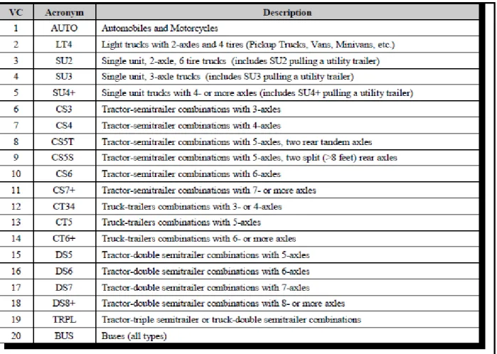
We now present a cost model for shipping commodities by truck. Shipping by trucks includes medium and heavy trucks as well as light trucks, pickups, and minivans. In this model, however, we assume that all transportation is performed by large trucks in class 8 (see appendix A).

The following units are used throughout this model with respect to the following quantities:

- Traveling distance: English system (miles) - Fuel volume: English system (gallons)

- Weight: English system (lbs, tons (1 ton = 2000 lbs)) - Cargo volume: English system (ft3)

- Temperature: English system (degrees Fahrenheit)

The model has two kinds of inputs—parameters and constants as shown in Tables 2 and 3. Parameters are model inputs that define the service to be provided—the commodity (group) that is shipped, how much is shipped, where it is to be shipped, and any additional requests. The constants define the industry environment for providing transportation services. They include the price of fuel, equipment costs, insurance costs, the current state of technology, and various regulations such as the maximum allowed driving time in a 24-hour period. The values of the constants are likely to change over time and should therefore be reviewed periodically.

The model is relatively broad in scope but still has some limitations. First, in the final form of this model we assume there is only one driver per truck. In other words, we do not account for the possibility that two or more drivers (e.g. a husband and wife) may share the same truck and thereby increase the total distance driven per day. However, we show later how to determine if another driver is necessary or not. Secondly, we do not consider multi-trailer units; we assume only one trailer per tractor. We do, however, allow a shipment to be carried by multiple trucks. Featured relations in this model are shown in Table 4.

TABLE 2 Parameters in Transportation Cost Model Parameter Description

Xo Shipment origin (5-digit zip code)

Xd Shipment destination (5-digit zip code)

Xc Commodity (5-digit SCTG code) or commodity group (2- to 4-digit SCTG code)

Xw Shipment weight (lbs)

Xtw Truck weight (lbs)

Xtemp Requested cargo temperature (degrees Fahrenheit)

Xtime Requested maximum journey time (hrs)1

Xtrailer Trailer and dock type

Xplu Packaging, loading, and unloading method (0 = no unloading service requested; 1 =

unloading service requested)

1

18 The total transportation cost is a function of the parameters. This total cost is comprised of the individual costs for fuel, labor, depreciation, maintenance, loading and unloading,

insurance, overhead, and extra expenses.

Total Cost = Cost(Xo , Xd , Xc , Xw , Xtemp , Xtime , Xtrailer , Xplu ) =

Fuel(Xo , Xd , Xc , Xw , Xtw , Xtemp , Xtime , Xtrailer , Xplu ) +

Labor(Xo , Xd , Xc , Xw , Xtw , Xtemp , Xtime , Xtrailer , Xplu ) +

Deprec(Xo , Xd , Xc , Xw , Xtw , Xtemp , Xtime , Xtrailer , Xplu ) +

Maint(Xo , Xd , Xc , Xw , Xtw , Xtemp , Xtime , Xtrailer , Xplu ) +

Load(Xo , Xd , Xc , Xw , Xtw , Xtemp , Xtime , Xtrailer , Xplu ) +

Insur(Xo , Xd , Xc , Xw , Xtw , Xtemp , Xtime , Xtrailer , Xplu ) +

Over(Xo , Xd , Xc , Xw , Xtw , Xtemp , Xtime , Xtrailer , Xplu ) +

19

TABLE 3 Constants in Transportation Cost Model

Constant Description Estimated values as of April, 2009

CmaxWt Truck capacity (lbs) Appendix A

CmaxVol Trailer inside volume (ft3) Appendix A

Cfuel$ Cost of fuel ($/gal) 2. 1

CoptSpd Truck speed that yields optimum fuel efficiency (miles/hr) 55

CmaxEff Truck fuel efficiency while traveling with empty trailer at

optimum speed for fuel efficiency (miles/gal)

7-7.5

CminEff Truck fuel efficiency while traveling with full load (by

weight) at optimum speed for fuel efficiency (miles/gal)

5-6

CspdLim Official truck speed limit on highway (miles/hr) 45-65

Chours Maximum allowed driving time for a single driver in any

24-hour period (hrs)

11

Cref Refrigeration unit fuel consumption per Fahrenheit degree

difference between outside temperature and requested cargo temperature per hr (gal/(degree*hr))

0.4

Cperish Commodity’s perishablity value (0-1) X

†† Cidle Average fuel consumption during idling (gal/hr) 1

Cwage Driver wage ($/mile) 0.40

ChthIns Annual cost of driver health insurance ($) 6000

Cpension Annual cost of driver pension plan ($) 6,500

CSocialMed Annual cost of driver social security tax and Medicare

tax ($)

7,650

Cannual Distance an average truck is driven annually (miles) 120,000

Cnew Cost of new tractor + trailer ($) 125,000

Clife Truck expected lifetime (years) 5

Csalv Truck salvage value at end of expected lifetime ($) 25,000

CmaintGM Truck general maintenance cost per mile for engine and

non-engine maintenance purposes ($/mile)

X†

CmaintT Truck tires maintenance cost per mile ($/mile) X

†† Cunload Average truck unloading cost ($/trailer) 40

CtrkIns Annual cost of full liability, collision, and theft insurance for

a truck ($/truck)

5,000

CcrgIns Cost of cargo damage insurance for a commodity with

maximum fragility level (= 1) per mile per $10,000 in value of the commodity (pro-rated for commodities with fragility levels less than 1) ($/truck-mile)

X†††

CothIns Annual cost of other insurance for a truck ($/truck) 5,000

COH Overhead and indirect cost ($/truck-mile) 0.17

Chaz Cost of shipping a commodity with maximum hazard level

(= 1) (pro-rated for commodities with hazard levels less than 1) ($/truck-mile)

20

TABLE 3 Constants in Transportation Cost Model (continuation)

Constant Description Estimated values as of April, 2009

CregLic Annual cost of vehicle registration and driver licensing

($/truck)

Appendix A (State of Indiana is used as an example )

†

Varies according to total truck shipment load.

††

Varies according to total truck shipment load, and total trailer and tractor tires .

†††

Theses values are according to commodity and shipper considerations.

TABLE 4 Featured Relations in Cost Model

Milwaukee approximation for heavy truck fuel consumption ”Total trip distance” †

𝑇𝐹𝐶 =

𝑊𝑠𝑙𝑖55 ∗ Dist (Xis − Xif) / [ 33,000 M 1.536 0.17 + 2.43_V 15 i=5 ] , speed < 55mph 𝑊𝑠𝑚𝑖55 ∗ Dist(Xis − Xif)/ [ _{1.53 ∗ 10−6} 1 ∗ M + 2.94 ∗ 10−5_{+ 1.94 ∗ 10}−13_{∗ M ∗ V}2 ] 4 𝑖=0 , speed ≥ 55 mph

Total shipping cost per truck †

Cost(Xo , Xd , Xc , Xw , Xtemp , Xtime , Xtrailer , Xplu ) =

𝐶_{𝑓𝑢𝑒𝑙 $} 𝐹𝑢𝑒𝑙𝑇𝑟𝑎𝑣 + 𝐹𝑢𝑒𝑙𝑅𝑒𝑓𝑟 + 𝐹𝑢𝑒𝑙𝐼𝑑𝑙𝑒 + 𝐿𝑎𝑏𝑜𝑟𝑊𝑎𝑔𝑒 + 𝐿𝑎𝑏𝑜𝑟𝐻𝑒𝑎𝑙𝑡𝑕𝐼𝑛𝑠 + 𝐿𝑎𝑏𝑜𝑟𝑆𝑜𝑐𝑖𝑎𝑙𝑀𝑒𝑑 + 𝐿𝑎𝑏𝑜𝑟𝑃𝑒𝑛𝑠𝑖𝑜𝑛 + 𝑑𝑖𝑠𝑡 𝑋𝑜, 𝑋𝑑 𝐶_{𝑎𝑛𝑛𝑢𝑎𝑙} 𝐴𝑛𝑛𝑢𝑎𝑙𝐷𝑒𝑝𝑟 + 𝑑𝑖𝑠𝑡 𝑋_𝑜, 𝑋_𝑑 (𝐶𝑚𝑎𝑖𝑛𝑡𝐺𝑀 + 𝐶𝑚𝑎𝑖𝑛𝑡𝑇 ) + (𝐶𝑢𝑛𝑙𝑜𝑎𝑑 )(𝑋𝑝𝑙𝑢) + 𝑇𝑟𝑘𝐼𝑛𝑠 + 𝐶𝑎𝑟𝑔𝐼𝑛𝑠 + 𝑂𝑡𝑕𝐼𝑛𝑠 + 𝐶_𝑂𝐻 (𝑑𝑖𝑠𝑡 𝑋𝑜, 𝑋𝑑 ) + 𝑅𝑒𝑔𝐿𝑖𝑐 + 𝐻𝑎𝑧 †

These relations built according to 2009 technologies for heavy trucks ―class 8‖

21

Model Setup

Let Speed be the average speed while traveling. The time spent idling, sleeping, on

breaks, and at rest stops is not considered here. Depending on driver preference, Speed might take the value Coptspd , Cspdlim , Cspdlim + 10, or any other value.

Let dist(Xo, Xd) be the trip distance.

Fuel

Let density(Xc) be the cargo density in lbs/ft3. This density can be derived from the

commodity type Xc. Let NumVeh be the number of trucks needed to haul the shipment. This quantity depends on whether shipment weight or shipment volume is the determining factor. In other words, we must determine whether the cargo will ―weigh out‖ a trailer before it ―cubes out‖ a trailer or vice versa. Note that 𝑋𝑤

𝐶𝑚𝑎𝑥𝑊𝑡 gives the number of trailers required based on a

consideration of shipment weight alone. Also, 𝑋𝑤/𝑑𝑒𝑛𝑠𝑖𝑡𝑦 𝑋𝑐

𝐶𝑚𝑎𝑥𝑉𝑜𝑙 gives the number of trailers

required based on a consideration of shipment volume alone. The number of trailers required based on a consideration of both shipment weight and volume is therefore the maximum of these two values rounded up to the nearest integer.

𝑁𝑢𝑚𝑉𝑒𝑕 = max

𝐶𝑚𝑎𝑥𝑊𝑡

,

𝑋𝑤/𝑑𝑒𝑛𝑠𝑖𝑡𝑦 𝑋𝑐

𝐶𝑚𝑎𝑥𝑉𝑜𝑙

In the case of palletized shipment using boxes or pallets, or a combination of both of them the pallet specification should be considered. To find out number of trucks required we need to know the number of pallets used. Let PallCap be the capacity of one pallet (lbs) and

NumPall be the number of pallets required for the shipment.

𝑁𝑢𝑚𝑃𝑎𝑙𝑙 =

𝑋

𝑃𝑎𝑙𝑙𝐶𝑎𝑝

Number of each kind of pallet inside any trailer depends on the inside trailer and pallet dimensions. Let PallTra be number of pallets that can fit inside the trailer while PaDim1,

PaDim2 and PalDim3 are the pallet dimensions and InTraDim1, InTrDim2 and InTrDim3 are

inside trailer dimensions. In many cases you can orient the boxes or the pallets inside the trailer in any direction to maximize number of pallets in the stack.

†

22

𝑃𝑎𝑙𝑙𝑇𝑟𝑎 = max

𝐼𝑛𝑇𝑟𝑎𝐷𝑖𝑚 𝑋

𝑃𝑎𝑙𝐷𝑖𝑚 𝑋

.

𝐼𝑛𝑇𝑟𝑎𝐷𝑖𝑚 𝑌

𝑃𝑎𝑙𝐷𝑖𝑚 𝑌

.

𝐼𝑛𝑇𝑟𝑎𝐷𝑖𝑚 𝑍

𝑃𝑎𝑙𝐷𝑖𝑚 𝑍

,

𝐼𝑛𝑇𝑟𝑎𝐷𝑖𝑚 𝑋

𝑃𝑎𝑙𝐷𝑖𝑚 𝑌

.

𝐼𝑛𝑇𝑟𝑎𝐷𝑖𝑚 𝑌

𝑃𝑎𝑙𝐷𝑖𝑚 𝑋

.

𝐼𝑛𝑇𝑟𝑎𝐷𝑖𝑚 𝑍

𝑃𝑎𝑙𝐷𝑖𝑚 𝑍

Number of trailers if the shipment is palletized is given by the following expression:

𝑁𝑢𝑚𝑉𝑒𝑕2 = 𝑚𝑎𝑥

𝑋

𝐶

,

𝑁𝑢𝑚𝑃𝑎𝑙𝑙

𝑃𝑎𝑙𝑙𝑇𝑟𝑎

According to the current technology used in today’s trucks, for a tractor plus empty trailer weighing around 20,000 lbs, the fuel efficiency is roughly 7.5 miles/gallon. For each additional 20,000 lbs of cargo hauled, the truck fuel efficiency decreases by about 1 mile/gallon.

This working paper developed its own heavy truck fuel approximation. The authors of this working paper call this formulation the Milwaukee Approximation for heavy truck fuel consumption.This approximation combines the most updated theoretical and empirical relations. The approximation has discontinuous equations and relates truck fuel consumption (mpg) to driving speed (mph).The energy required to run a truck is given in equation 1.

F

=

A

+

Bv

+

Cv

………….(1).

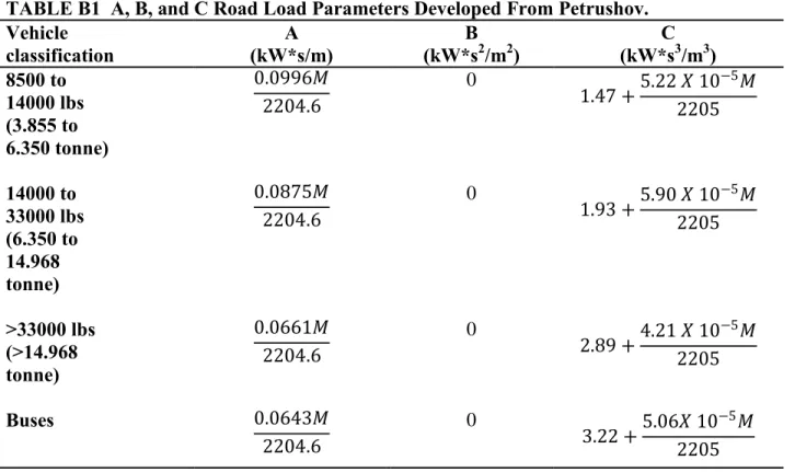
Coefficients A, B and C are defined according to Giannelli et al. (2005). Since 55 mph is the most fuel efficient driving speed according to most of the theoretical resources and the available practical data, equation 1 is used for speeds of 55 mph and above. The equation has been converted from its original units of Newtons to miles per gallon (MPG) as in equation 2. See appendix B for more details about our calculations and conversions.

MPG = 1 / [(1.53*10

*M) + (2.94*10

+1.94*10

*M)*V

]…………(2)

In equation 2, M is the total truck mass in lbs, and V is the truck driving speed in mph.

To find MPG for a speed less than 55 mph, Papacostas’s textbook (Transportation and Engineering Planning, 2000) has been used. Papacostas reports a relation from the early 1980s between MPG and speed when the speed is less than 35 mph. The data in Factors Affecting Fuel Economy paper (Good Year, 2003) was used to update Papacostas’s relation and extend it to include driving speeds less than 55 mph as in equation 3.

23 In equation 3, V is the speed in miles per hour.

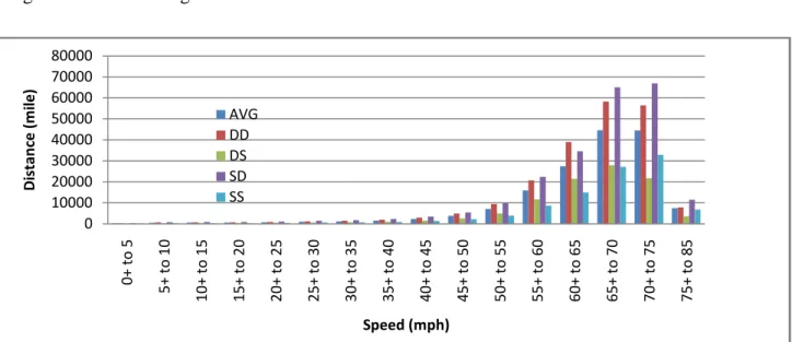
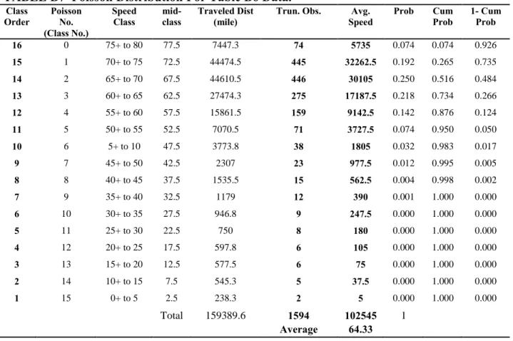
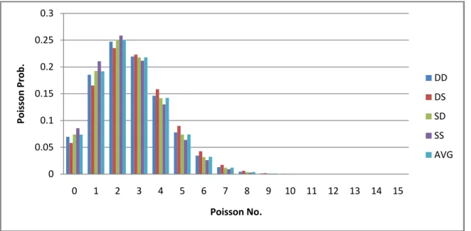
The model created in this paper divides driving speeds into 16 classes, each class being a different 5-mph interval, starting with 0 mph and ending at 80 mph. Class 0 pertains to speeds from 75-80 mph, class 1 pertains to speeds from 70-75 mph, and so on so that class 15 pertains to speeds from 0-5 mph. The probability (i.e. relative amount of time) the driver drives at each of these speed classes is found using data published in the Transportation Energy Data Book edition 2008-2009 as a part of a vehicle duty cycle project (Oak Ridge, 2008). These data show the distance traveled in each speed class. A reverse Poisson distribution (with parameter

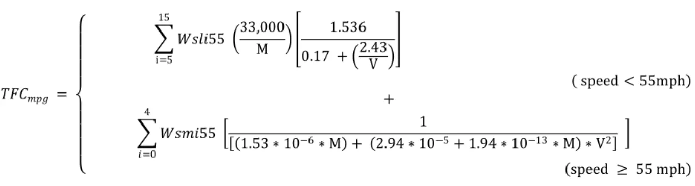
depending on the average driving speed) is the most appropriate distribution that fits these data. For more details see Appendix B. The total fuel consumption for any trip is found using the relation below. 𝑇𝐹𝐶 = 𝑊𝑠𝑙𝑖55 ∗Dist (Xis− Xif) / [ 33,000_M 1.536 0.17 + 2.43_V 15 i=5 ] speed < 55mph + 𝑊𝑠𝑚𝑖55 ∗Dist Xis− Xif _{1.53 ∗ 10}−6_{∗ M + 2.94 ∗ 10}1 −5_{+ 1.94 ∗ 10}−13_{∗ M ∗ V}2 4 𝑖=0 speed ≥ 55 mph Where,

TFC : Truck fuel consumption (gallons).

M: Total truck and trailer mass (lb), M = Xtw + Xw V: Driving speed (mi/hr)

Wsli55: The probability of driving at speed class i, when i > 4 (less than 55 mph).

Wsmi55: The probability of driving at speed class i, when i ≤ 4 (more than 55 mph).

Dist (Xis-Xif): The distance traveled at velocities in speed class i, which has a minimum speed of

Xis and a maximum speed of Xif .

Average speed (AvgSpeed) in this model is calculated by any of the following expressions, according to the user’s data and requirements. Let Dist (Xis-Xif) be the distance

traveled by speed class i, which starts with speed more than Xis and ends by speed equal or less

Xif mph, and Time (Xis-Xif) is the time consumed in traveling by speed class i.

AvgSpeed

=

Dist (Xis−Xif) Time (Xis −Xif ) 15

0 Or,