MAPer: A Multi-scale Adaptive Personalized Model for
Temporal Human Behavior Prediction
Sarah Masud Preum
University of Virginia Charlottesville, Virginia 22904[email protected]
John A. Stankovic
University of Virginia Charlottesville, Virginia 22904[email protected]
Yanjun Qi
University of Virginia Charlottesville, Virginia 22904[email protected]
ABSTRACT
The primary objective of this research is to develop a simple and interpretable predictive framework to perform temporal modeling of individual user’s behavior traits based on each person’s past observed traits/behavior. Individual-level hu-man behavior patterns are possibly influenced by various temporal features (e.g., lag, cycle) and vary across tempo-ral scales (e.g., hour of the day, day of the week). Most of the existing forecasting models do not capture such multi-scale adaptive regularity of human behavior or lack inter-pretability due to relying on hidden variables. Hence, we build a multi-scale adaptive personalized (MAPer) model that quantifies the effect of both lag and behavior cy-cle for predicting future behavior. MAper includes a novel basis vector to adaptively learn behavior patterns and cap-ture the variation of lag and cycle across multi-scale tempo-ral contexts. We also extend MAPer to capture the inter-action among multiple behaviors to improve the prediction performance.
We demonstrate the effectiveness of MAPer on four real datasets representing different behavior domains, including, habitual behavior collected from Twitter, need based behav-ior collected from search logs, and activities of daily living collected from a single resident and a multi-resident home. Experimental results indicate that MAPer significantly im-proves upon the state-of-the-art and baseline methods and at the same time is able to explain the temporal dynamics of individual-level human behavior.
Keywords
Time series prediction; Temporal human behavior modeling
1.
INTRODUCTION
Regular human behaviors are constantly being captured in virtual platforms ( e.g., social media, search logs) as well as in physical platforms (e.g., smart phone, smart watch) [16]. The vast amount of individual user data generated by these platforms facilitates modeling the temporal footprint
Permission to make digital or hard copies of all or part of this work for personal or classroom use is granted without fee provided that copies are not made or distributed for profit or commercial advantage and that copies bear this notice and the full cita-tion on the first page. Copyrights for components of this work owned by others than ACM must be honored. Abstracting with credit is permitted. To copy otherwise, or re-publish, to post on servers or to redistribute to lists, requires prior specific permission and/or a fee. Request permissions from [email protected].
CIKM’15,October 19–23, 2015, Melbourne, Australia.
c
2015 ACM. ISBN 978-1-4503-3794-6/15/10 ...$15.00. DOI: http://dx.doi.org/10.1145/2806416.2806562.
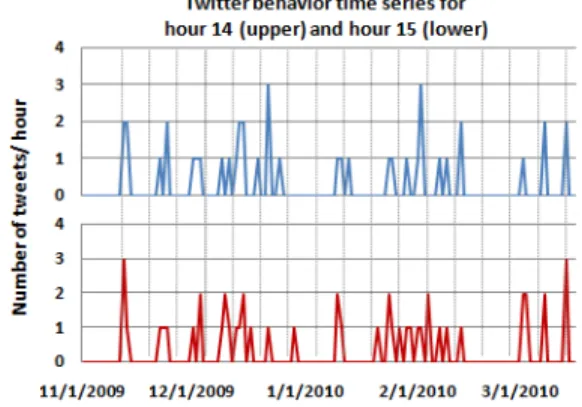
Figure 1: A Twitter user often tweets at hour 14 and hour 15 at the same day. This depiction from real data suggests an impact of lag on tweeting behavior, i.e., the behavior at hour 14 is followed by the behavior at hour 15.
of different human behaviors. Accurate and explanatory temporal behavior models can serve as the building block of several useful applications.
For example, predicting when an online user is going to be active (e.g., searching a query, posting a tweet) can be use-ful for targeted advertising (e.g., finding peak social hours to maximize visibility of content among target audience) [6], churn prediction (i.e., predicting users who are likely to leave a service provider) [27], and temporal user profiling [1, 11]. Similarly, a predictive model that can model human behav-iors in the context of daily activities (e.g., sleeping, cooking, or eating) is extremely useful for functional assessment of el-derly people [9] and designing behavior intervention for reha-bilitation [26]. Scott et al. demonstrated that dynamically predicting room occupancy and energy usage patterns of its residents enable efficient designing of smart thermostats and thus save energy costs significantly [23]. Explanatory predic-tive models can serve end users who use smart phones and smart watches for self monitoring: a sleep monitoring ap-plication that builds explanatory predictive models of sleep pattern can help the user to detect sleep anomaly and sug-gest sleep time.
This paper focuses on a data-driven modeling of temporal human behavior at a single individual level. Our goal is to build an accurate and interpretable temporal behavior model that can serve as a building block for the motivating examples presented above.
Individual-level temporal behavior is often influenced by three major temporal features: (1) temporal smoothness (i.e., lag), (2) behavior rhythms (i.e., cycle), and (3)
interac-tion among multiple behaviors. Temporal smoothness refers to lag phenomenon: behavior at timetcan be influenced by the behavior at time (t−1) (Figure 1). Behavior rhythm refers to the repetitive habits of a human. For instance, some online users frequently post tweets on Friday night (i.e., cy-cle length is 7 days). Moreover, often the interaction among multiple behavior traits/activities needs to be captured to model a single behavior, e.g., watching TV until late night can delay sleep time. Quantifying the effects of these fea-tures on a specific behavior of an individual is challenging, because they vary with multi-scale temporal contexts (e.g., specific hour of the day or day of the week). Such as, working people may prefer watching TV for a longer duration dur-ing weekend nights rather than durdur-ing weekday morndur-ings. Here, the lag length is changing due to the change in tem-poral context from a weekday morning to a weekend night. To address such personalized temporal dynamics, we need a modeling approach that dynamically adapts with such vari-ation of features over multiple time scales.
The existing time series prediction models are too general to be applicable in this context. With regard to the com-putational behavior modeling methods, the most relevant existing study is from Zhu et al. where they predict user ac-tivity level in social media [27]. But their modeling of tem-poral behavior dynamics is limited to reducing the impact of out-of-date training data. Another work uses Bayesian networks to predict future activity based on current activity in a home setting [20]. Neither of these works quantify the effect of variation of the temporal features across multi-scale temporal contexts (e.g., daily, weekly).
The main contributions of this paper are following. (i) We build a multi-scale adaptive personalized model, namelyMAPer, that models regular temporal human be-havior by capturing the effects of three temporal features: lag, cycle, and interaction among multiple behaviors. (ii) We introduce a novel approach to capture the variation of these behavior features across multi-scale temporal contexts and learn adaptively. (iii) Our performance analysis demon-strates the overall effectiveness of MAPer as compared to multiple baselines and a state-of-art time series prediction model (SARIMA). Using behavior data collected from Twit-ter [7], search logs [21], and two smart homes [3, 13], we show the effectiveness of the key parts of the model, demon-strate the value of personalization, and perform a sensitivity analysis along three dimensions: training set size, temporal scale, and order of lag. These experiments show MAPer reduces prediction error by about 15%, 31% and 10% over the state-of-art SARIMA model for Twitter, search log, and a single resident smart home data, respectively. (iv) An-other key value of our solution is its explanatory capability. As MAPer uses a linear model for prediction based on only observed behavior, it has higher interpretability over other predictive models that are non-linear or rely on unobserved variables (e.g., state space model or hidden Markov model).
2.
PROBLEM FORMULATION
2.1
Extracting Discrete Time Series from
Tem-poral Behavior Data Stream
We useH(t) to represent a given behavior data with cor-responding time stamp spanning over a total stream length
T. We divideT into a set ofn equal length time intervals
t1, t2, . . . , ti, . . . , tn. Then we summarizeH(t) over each
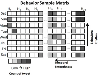
in-Figure 2: An example of behavior sample matrix representa-tion: demonstrating lag and cycle for modeling an individual user’s behavior in the context of Twitter usage. The cells are darkened in proportion to the number of tweets at the corresponding time interval.
terval to obtain behavior sampleHs(s, ti), such thatHs
ap-plies a summarizing processsover the behavior of intervalti.
The summarizing processscan be frequency/average/length of some countable behavior measure. With this process we get a discrete series of n behavior samples: Hs(s, t1),
Hs(s, t2),. . . ,Hs(s, tn) For example, consider a set of tweets
from a Twitter useru, where each tweet has its correspond-ing time stamp. After sortcorrespond-ing the tweets accordcorrespond-ing to their increasing time stamp, we find the total window length T
that spans from the starting time stamp to the ending time stamp. Assume there aren different days in T. Next, we divide T into hourly/daily/weekly intervals. If the chosen interval ishour and the chosen summarizing process istotal count of tweetsthen the behavior sample will betotal count of tweets per hour. In this case, the length of the behav-ior sample time series will ben×24, since we divide each day into 24 hours. The choices of interval and summarizing process depend on a specific application requirement.
We denote the time seriesHs(s, ti) asyiin the rest of the
paper. In addition, we denoteyi for an activity1 kof a user
(e.g., an activity of daily living) asykt. Our goal is to predict
yk
i based on it’s previous values i.e.,yk1, yk2, . . . , yki−1.
Essentially, a more accurate notation would be yk,ut to
indicate modeling specific activity k from an individual u. Instead, we use the simplified notationyk
t since we do not
consider interaction among multiple users for predicting fu-ture activity of a single user.
2.2
Behavior Sample Matrix Generation
After generating the discrete time series from historical longitudinal behavior data of a user (uk), we create
corre-sponding behavior-sample matrix (M) to extract features corresponding to lag, cycle, and interaction with other be-haviors. This matrix representation encodes the temporal patterns of behavior concisely. Specifically, each row ofM
represents a day (di) and each column of M represents an
hour (hj). The content of a cell Mi,jk is the sample of a 1We use the terms activity and behavior interchangeably in
behaviork from a useru on daydi and hour hj. In other
words,Mi,jk represents the intensity of overall activity level
of the user at thej-th hour of thei-th day.
Figure 2 demonstrates a Twitter behavior sample matrix where the behavior sample is the count of tweets per hour. It appears this particular user is most active during weekend nights. Tweets generated at hour 14 might act as a lag feature to tweets generated at hour 15. The Twitter user usually tweets on hour 24 during weekends. So there is a possible cycle of this behavior that repeats on weekends. As shown in Figure 2, the contents of same columns contribute to behavior rhythm or cycle and the contents of same rows contribute to temporal smoothness or lag.
This matrix representation highlights the lag and cycle properties of regular human behavior and is easily gener-alizable to represent more coarse or granular time scales. After generating behavior sample matrix, we build a gen-eral temporal model for behavior prediction that extracts the temporal features from this matrix.
3.
MULTI-SCALE ADAPTIVE
PERSONAL-IZED MODEL
In this section we present incrementally the formation of the MAPer model. Since MAPer combines lag, cycle, and interaction among multiple behaviors across multiple tem-poral scales, we first describe extracting lag feature(s) and then incrementally add features culminating in the complete model in Section 3.1.4.
3.1
Extracting Features for Temporal
Behav-ior Prediction
3.1.1
Temporal Smoothness/Lag Features
For the purpose of forecasting the lag features can be rep-resented using auto regression (AR), a standard linear time series forecasting technique. An l-th order auto-regressive model for predicting thet-th item of a behavior time series time series is described as,
ˆ yt= l X i=1 αi·yt−i+c+ (1)
where α1, α2, . . . , αl are lag parameters to learn, c is a
constant, and the random variablerepresents white noise [12]. The coefficient value ofαi quantifies the effect of the
i-th lag component for the current time point. Referring to Figure 2, for a cellMi,jk in a behavior time series matrixMk,
we considerMk
i,j−1as the lag of order 1,Mi,jk−2as the lag of
order 2, and so on. We also wrap the matrix to extract lag features for early hours of a day. Such as, when predicting for hour 1 of a day and considering a lag of order 4, we extract lag features from hour 21 to hour 24 of the past day.
3.1.2
Behavioral Rhythm/Cycle Features
Human behaviors often demonstrate cyclic pattern, such as, cooking meal on every Friday night (i.e., the cycle is 7 days). To capture the behavior rhythm effect, we add a cycle component in Equation 1. The derived model for a single individual is presented below.
ˆ yt= l X i=1 αi·yt−i+ c X j=1 βj·yt−cj +c 0 + (2)
Here, the value of the coefficientβj quantifies the effect of
j-th cyclic component on the current time point of interest. If the cycle of a behavior time series is found to be 7 days, we will use Mk
3,16 as a cycle feature to predict the value
of M10k,16. We describe the method of selecting cycles of a
behavior time series in Section 3.2.
In the rest of the paper, we refer to the model correspond-ing to Equation 2 as the auto regression with cycle compo-nent (AR-C) model.
3.1.3
Interaction Features
So far for predicting future values of time series of activity
k (i.e., ytk), we have extracted features from only the time
seriesyk
t. But often time series of one activity can influence
another from the same user as the corresponding activities interact with each other. We define such interaction of hu-man behaviors/activities in terms of co-occurrence. We hy-pothesize that, if two activities are frequently observed con-secutively, the former activities can influence the prediction of the later for which theyinteract. For instance, watching TV and using internet until late night often delay sleeping. In this case,watching TV andusing internetare interacting with sleeping. Similarly, having a meal is usually followed by washing dishes. To consider such interactions among ac-tivitykand other activities, we update equation 2 as below.
ˆ ytk≈ Lk X i=1 αki ·y k t−i+ Ck X j=1 βjk·y k t−cj+ X k0∈S Lk0 X l0=1 Wl(0k,k0)·y k0 t−l0 (3) Here,S is a set of activities of a useruand k6=k0 such that activity k0 precedes activity k and interacts with it.
Lk0 refers to the length of lag that we are considering for
the behavior time seriesyk0
t . Note that we omitc
00
+from Equation 5 and subsequent equations to simplify notations. Unlike Equation 2, Equation 3 models an individual’s sin-gle activityk using historical values ofkand a set of other activities (i.e.,k0s) that influencek.
3.1.4
Multi-scale Adaptive Features
For regular daily human behavior the two most common temporal contexts of behavior are day of the week and hour of the day. Often behavior varies over such multi-scale tem-poral contexts. The lag length, cycle, and amount of interac-tion vary with the temporal contexts too. Such as, the order of lag of watching TV is likely to vary from morning to night for working class people, as they have to leave home early in the morning. Here the lag is varying with hour of the day. Similarly, it can vary with day of the week. Therefore, we need a feature representation to encode such multi-scale variation and adapt the prediction model dynamically.
Hence, we introduce a discrete binary vector representa-tion describing multi-scale temporal contexts whose length is determined by the corresponding scale (e.g., hour of the day or day of the week) and whose value is determined by the current time stamp. Specifically, hour ican be repre-sented as a 24-dimensional binary vector with a series of (i−1) zeroes followed by an one and (24−i) zeroes. Thus, hour 3 can be represented by a series of two zeroes followed by an one and 21 zeroes. The corresponding vector B3 is
[00100. . .0], where |B3|= 24. Similarly, we obtain a basis
We denote the combination of daily basis vector and weekly basis vector asB~d, ~Bw. We add this basis vector
represen-tation in Equation 3 to represent the multi-scale temporal context. ˆ ytk≈ Lk X i=1 αki ·y k t−i+ Ck X j=1 βkj·y k t−cj+γ k ·(B~d, ~Bw) +X k0∈S Lk0 X l0=1 Wl(0k,k0)·yk 0 t−l0 (4)
We use the model corresponding to Equation 4 when we consider interaction between multiple streams of behavior. Otherwise, we use the following model.
ˆ ytk≈ Lk X i=1 αki ·y k t−i+ Ck X j=1 βkj·y k t−cj+γ k ·(B~d, ~Bw) (5)
It should be noted that unlike lag and cycle features, the value of (B~d, ~Bw) is not unique for all yt where t ∈
1,2, . . . , n. (B~d, ~Bw) is same foryiand yj if they represent
same day of the week and same hour of the day. This is nec-essary to encode the temporal context of behavior: behavior samples from similar context share similar features. Equa-tion 4 captures the effect of temporal smoothness, behav-ior rhythm, interaction, and multi-scale temporal contexts using parametersαi,βj,γ, and basis vectors (B~d, ~Bw),
re-spectively. This model is personalized for each user and is customized for each activity of the user. In addition, the basis vector representation enables the model to learn adap-tively across multi-scale temporal contexts. Hence we denote the model corresponding to Equation 4 as the Multi-scale
AdaptivePersonalized (MAPer) model.
With different combination of basis vectors, we have two variations of MAPer: (i) daily scale adaptive personalized (DAPer) model that uses only daily basis vector (B~d) and
(ii) weekly scale adaptive personalized (WAPer) model that uses only weekly basis vector (B~w). MAPer uses both daily
and weekly basis vectors. MAPer can be also generalized to add more coarse/granular temporal contexts.
3.2
Feature Selection
Cycle Features: The cycle of a behavior can vary across individual users and individual activities. We extract the cy-cle length of a behavior time series by applying discrete Fast Fourier Transform (FFT) analysis, a spectral decomposition technique where we treat the time series as an input signal. Although there are other time series decomposition tech-niques including piecewise polynomial, symbolic, wavelets, etc. [24], they are out of scope of this paper. We derive a set of frequencies from the FFT analysis and choose the highest
C frequencies as the relevant cycle features, where the fre-quencies are sorted according to their amplitudes. We plug in these C frequencies as the cycle features in the models corresponding to Equation 2 to Equation 5.
Interaction Features: Considering all activities for mod-eling interaction can introduce noise rather than signal and increase the feature space prohibitively, since only a subset of behaviors interact with each other usually. To select a subset of activities that interact with our target activityk, we propose a frequent item-set mining approach. Specifi-cally, for each day we sample every two hours and create
an itemset of activities that took place during that window. We empirically set the window length to two hours. We do not use a strict window to create itemsets as (i) it results into large number of unique itemsets (i.e., occur only once), (ii) it can not capture fluctuation of routine: one may fre-quently have dinner at anytime between 7.30pm to 8.30pm. After all the itemsets are generated over the training set, we generate the closed itemsets2 using ECLAT [5], a fast
algo-rithm for frequent item set mining. For each activity of our interest, we sort other activities that appear in the closed itemsets based on how frequently they co-occur. Finally, for each activity k we use the top three activities derived from the closed item set such that they precede thek-th ac-tivity. The interaction features for activityk are extracted from these three activities according to Equation 4. Using frequent itemset mining for interaction features is scalable as the number of candidates (i.e., ADLs) for interaction is limited in our case.
4.
CONNECTING TO PAST STUDIES
Although the exact problem we are trying to solve is unique in the literature, there are various relevant areas of existing research as presented below.
Time series forecasting: For the task of time series prediction, the existing algorithms can be broadly catego-rized as parametric and non-parametric approaches. Para-metric approaches assume the underlying stationary process has a structure which can be estimated using a number of parameters. Hence, these methods normally fit a statisti-cal model on the time series data and have better inter-pretability. The Autoregressive Integrated Moving Average (ARIMA) model [15] is used to forecast a stationary time series3. The ARIMA model predicts a stationary time
se-ries (yt) using lags of the dependent variable (yt−l) and
lags of forecasting error (et = yt −yˆt). A non seasonal
ARIMA model is expressed as ARIMA(p,d,q) where p,d, and q are the model parameters corresponding to the num-ber of auto-regressive terms, the numnum-ber of nonseasonal dif-ferences needed for stationarity, and the number of lagged forecast errors used in the prediction equation. SupposeYt
denotes the d-th difference ofyt, i.e., ifd= 0 thenYt=yt,
if d = 1 then Yt=yt−yt−1, and so on. Then the general
forecasting equation for the ARIMA model is ˆ Yt≈µ+ l X i=1 φi·Yt−i+ l X i=1 θi·et−i (6)
The ARIMA model is one of the most general time series forecasting models as many forecasting models are merely a special case of ARIMA model. For instance, ARIMA(l,0,0) is the l-th order auto-regressive model expressed as Equa-tion 1. A seasonal ARIMA (SARIMA) model is a state-of-art parametric model of time series forecasting. It uses seasonal lag and differencing to fit the seasonal pattern. The SARIMA model can be expressed as ARIMA (p,d,q)×
(P,D,Q), where P, D, and Q denote the number of seasonal autoregressive terms, the number of seasonal differencing, and the number of seasonal moving-average terms.
2An itemset is closed if none of its immediate supersets has
the same support as the itemset.
3A time series is stationary if its statistical properties are
constant over time. A non stationary time series can be made stationary by differencing and non-linear transforma-tion (if required).
On the other hand, nonparametric approaches (e.g., neu-ral network based local forecasting models) approximate the underlying structure of the stationary process that generates the time series without making any structural assumption. A comprehensive survey on time series forecasting can be found in [8]. There are also several variations of vector au-toregressive methods that aim at multi-dimensional time se-ries forecasting [18].
Activity Prediction: Although a lot of works from com-puter vision and sensing community focus on activity recog-nition, the problem of daily activity prediction is largely unexplored. A recent work [20] proposes an activity pre-diction approach using Bayesian network. Unlike us, they model the problem as a multi-label classification and predict activity label and relative start time using current activity label, location, and temporal context. Although they con-sider daily and weekly context of behavior, their approach does not quantify the effect of different temporal features and lacks explanatory power. Pentland et al. propose that some human behaviors (e.g., driving, running) can be de-scribed as a set of dynamic models (e.g., Kalman filters) sequenced together by a Markov chain. However, as their application domain involves more granular behavior, it does not require quantifying the effect of cycle on behavior or how lag/cycle varies with multi-scale temporal contexts.
Zhu et al. focus on predicting user activity level in social networks to facilitate churn prediction (i.e., identify users who are likely to leave a service) [27]. They build a person-alized and socially regularized time decay model based on logistic regression to capture effects of user diversity, social influence on future activity level. A novel approach of ac-tivity prediction was proposed in [25]. They predict a set of future popular activities by analyzing textual content of Twitter posts using keyword matching. Unlike other works [20, 27], they focus on aggregated behavior rather than indi-vidual behavior. Although these research focus on behavior prediction, unlike us they do not explicitly quantify the ef-fect of different temporal factors (e.g., lag, cycle) on regular human behavior.
Modeling Temporal Behavior: Recently, the tempo-ral modeling of online user population has been extensively studied in order to improve query search performance [22, 4, 17], to understand and model content generation in so-cial networking sites [1, 2], and to model mobile behavior of users [10, 19].
For example, aiming to improve the query auto-suggestion and the ranking results, Radinsky et al. recently developed a temporal modeling framework that predicts temporal pat-terns of aggregated web search behavior [22]. Specifically, they model temporal features, like, trend, periodicity, and sudden spikes of queries by using dynamic state space els. Although their work is similar to ours in terms of mod-eling behavior based on temporal features, they focus on temporal modeling of search queries, while our study fo-cuses on directly modeling the temporal behavior of humans. Baskaya et al. analyzed the effects of a set of search-related human behaviors (e.g., formulate a query, scan, click a link) on retrieval performance [4]. In [17] the authors studied how search behaviors of users evolve over time, e.g., long term users demonstrate more complex behavior than newbies.
In addition to improving query based content-search, tem-poral modeling has also been explored to analyze user be-havior in social media or on content sharing platforms. Abel
Name Entities Span Domain
Search log 1307 users 3 months Need based behavior Twitter 1274 users 5 months Habitual behavior ARAS 27 ADLs 1 month Multi-resident home HOLMES 14 ADLs 3 months Single-resident home
Table 1: Summary of datasets used for evaluation. et al. demonstrated how temporal profiling of Twitter users based on their shared contents facilitates personalized news article recommendation [1]. Although these previous studies mostly analyzed user generated textual contents for ing the temporal dynamics, our proposed temporal model-ing of individual-level human behavior could facilitate their goals as well.
5.
EXPERIMENTAL SETUP
5.1
Data
To evaluate the effectiveness and generality of our model we use four benchmark datasets each representing different aspects of human behavior. The datasets are summarized in Table 1. The details are described below4.
Search Log Data Representing Need Based Behavior
We use AOL search log data [21] for predicting temporal query search behavior. This dataset consists of around 20M web queries collected from 650k users. The data was col-lected for over three months starting from March 2006 to May 2006. The dataset includes anonymized user ID, search query, time stamp of query, and click information (whether a search result was clicked or not). The data is sorted by anonymous user ID and is sequentially arranged according to their time stamps. We have used a subset of this dataset containing 1307 unique users so that each user has a search log spanning 60 days. In our sampled dataset there are 449,423 unique queries in total. However, from our experi-ments we discover that our modeling approach is generaliz-able to other cases where the training phase is as small as 2 weeks (Section 6.3.1).
We consider number of unique queries per hour as the be-havior sample and generate a normalized bebe-havior sample matrix as described in Section 2.2. Other choices of be-havior samples include number of queries, number of clicks, duration of a session. Also, the temporal resolution of the interval (i.e., hour) can be adjusted to different granularity (e.g., week, day).
Twitter Data Representing Habitual Behavior
We use a Twitter dataset [7] for predicting users’ temporal social media behavior. It consists of 121,022 users and more than 9 million time-stamped tweets that were collected from September 2009 to January 2010. However, it does not in-clude any re-tweet and follow relationships. We sample the dataset to obtain the users who have Twitter posts spanning over at least 120 days. In total we obtain 1,275,709 tweets from 1,274 Twitter users for evaluating our predictive model. We consider number of tweets per hour as the behavior sample. Alternatively, one can use number of Twitter mes-sages, number of re-tweets, duration of Twitter session, or a weighted combination of these as a behavior sample. The
4
generation of a Twitter behavior sample matrix is similar to the generation of a search log behavior sample matrix.
ARAS: ADL Data from a Multi Resident Setting
We consider Activities of Daily Living (ADL) data as the behavior captured from physical world where each activity corresponds to a behavior.
We use the ARAS smart home project [3] dataset as a multi-resident ADL dataset. It contains labelled sensor data from a system deployed in a smart home of 2 residents. This dataset has 27 annotated activities of daily living for each user. It contains start time and end time of each activ-ity. With a preference to model and predict health related behaviors, we focus on 5 behaviors from each user. They are: sleeping, snacking, having breakfast, lunch, and dinner. However, for resident 2, the number of samples for having breakfast, lunch and dinner are too few. So we model 7 activities for 2 users in total: sleeping of both residents, snacking of both residents, and breakfast, lunch, and dinner of resident 1.
HOLMES: ADL Data from a Single Resident Setting
We use HOLMES dataset as a single resident ADL dataset [13]. We use three months data from this dataset. It con-tains 15 annotated activities from which we model the fol-lowing health related activities: sleeping, breakfast, lunch, dinner, snack, shower, and cooking.
While in case of the Twitter data and the search log data we model each user separately, in case of the ADL data we perform forecasting of each activity of each user separately5.
Unlike the Twitter or search log data, we use the duration of an activity as the behavior sample instead of count of activ-ity since most of the ADL take place only once per interval. We sample each activity duration every half an hour for each day to form a time series of duration of each activity. Later, we vary the temporal resolution/scale to demonstrate the effect of temporal resolution on the prediction accuracy. We normalize the behavior sample matrix,M such that if activ-ityk takes place over the whole span of intervaljon dayi, thenMk
i,j contains 1; if activityak takes place over half of
the span of interval jof day i, then Mi,jk contains 0.5 and
so on.
5.2
Comparing with Baseline Methods
1. Moving Average(MA): As one of the simplest time series forecasting method, the moving average method pre-dicts average ofl lag values as the next value. We modify the original moving average model to include the effect of cycle. Specifically, the prediction atytis the average of alll
lag components and allccyclic components. Using our be-havior sample matrix, the lag components are selected from
l previous columns of the same row and the cycle compo-nents are selected fromcprevious rows of the same column. Mathematically, ˆ yt≈0.5× Pl i=1yt−i l + Pc i=1y(t−i∗24) c ! .
In our experiments we setl= 4 hours andc= 14 days. To compare the performance of MAPer with a non-parametric
5
Given a Twitter dataset that annotates different activities of a user (e.g., tweeting, re-tweeting, sending message), we can model each ac-tivity of a Twitter user separately too.
baseline method that considers both lag and cycle, we use this method.
2. Auto regression with Cycle Component( AR-C): Equation 2 refers to this baseline method.
To compare the performance of MAPer with a parametric baseline method that considers both lag and cycle, we use this method. It is also used to highlight the effectiveness of adaptive learning.
5.3
Comparing with state-of-art
We compare MAPer with the SARIMA model, a para-metric state-of-art forecasting model described in Section 4. We use an R implementation of SARIMA model provided in [14]. For parameter estimation of SARIMA model, we use a function that conducts a search over all possible models and return the best model according to AIC value. We use this model to explore the predictive power of MAPer across different behavior domains.
For the SARIMA model and MAPer, we perform two pa-rameter estimation settings: global and local. In general, we divide a chronologically sorted behavior dataset into train-ing and testtrain-ing sets. For global parameter estimation, we estimate the parameters only once using the full training set. But for local parameter estimation, we take a sliding window approach to form a separate training set for each point of test set. Specifically, for predictingi-th point in the test set, we construct the training set from (i−w) to (i−1) point wherewis the length of the sliding window.
5.4
Response Variable and Metrics
We evaluate our model mainly in a regression setting to predict the future intensity of a behavior marker based on its historical samples. In this setting, the content of each cell of behavior sample matrix acts as a response variable (yi)
where yi ∈[ 0,1] . The features described in Section 3 act
as the predictor variables. We measure the performance in terms of two standard evaluation metrics: mean square error (MSE) of prediction and Pearson correlation (PC) between the actualyand the predictedy.
We compare the baselines described in Section 5.2 with MAPer and show how effective the various features (de-scribed in Section 3) of MAPer are. We also evaluate the ef-fectiveness of (i) multi-scale adaptive features, (ii) personal-ized modeling, and (iii) interaction among activities. While comparing different methods, we set the corresponding pa-rameters to default values. Later, we perform sensitivity analysis by varying its hyper-parameters.
6.
EXPERIMENTAL RESULTS
6.1
Effectiveness of MAPer
6.1.1
Comparing with Baseline MethodsIn this section we compare the performance of MAPer with two baseline methods (Section 5.2). Referring to Ta-bles 2 and 3, MAPer outperforms all baseline methods in terms of MSE for search log, Twitter, and HOLMES data. MAPer increases the Pearson Correlation at least 1.5 times when compared to the baseline methods for all of the datasets. This highlights the significance of using tempo-rally adaptive learning method where the significance of lag and cycle features varies over time.
Baseline Methods state-of-art Multi-scale Adaptive Methods % Improvement Dataset MA AR-C Global SARIMA Local SARIMA Global MAPer Local MAPer over state-of-art Search log 0.046 0.045 0.065 0.048 0.045 0.041 14.6
Twitter 0.056 0.052 0.073 0.065 0.049 0.045 30.7
ARAS 0.032 0.017 0.042 0.011 0.018 0.016
-HOLMES 0.021 0.001 0.082 0.001 0.001 0.0009 10
Table 2: Comparing different methods in terms of meanMSE. The best performing (statistically significant) results are shown in bold. The right-most column shows the performance improvement of MAPer over the state-of-art (Local SARIMA). Local models outperforms global models and MAPer results into the lowest prediction error.
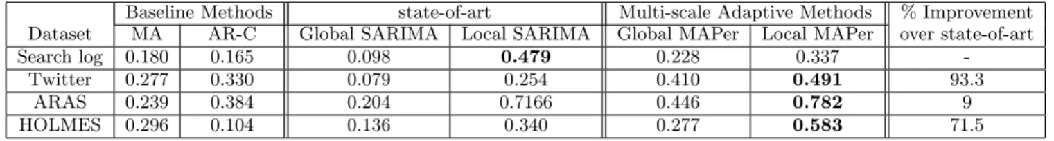
Baseline Methods state-of-art Multi-scale Adaptive Methods % Improvement Dataset MA AR-C Global SARIMA Local SARIMA Global MAPer Local MAPer over state-of-art
Search log 0.180 0.165 0.098 0.479 0.228 0.337
-Twitter 0.277 0.330 0.079 0.254 0.410 0.491 93.3
ARAS 0.239 0.384 0.204 0.7166 0.446 0.782 9
HOLMES 0.296 0.104 0.136 0.340 0.277 0.583 71.5
Table 3: Comparing different methods in terms of meanPearson Correlation. MAPer outperforms the SARIMA model for all datasets except the search log data.
6.1.2
Comparing with SARIMATables 2 and 3demonstrate that the local model out-performs the global model for all four datasets in case of both the SARIMA model and MAPer. This highlights the dynamic pattern of human behavior. In subsequent sections we use only the local estimation approach, i.e., MAPer refers to local MAPer.
In terms of MSE, MAPer with local parameter estimation outperforms SARIMA for both online behavior dataset and for HOLMES dataset. Specifically, it reduces MSE from the SARIMA model by 14.6%, 30.7%, and 10% for search log, Twitter, and HOLMES dataset, respectively. This perfor-mance improvement is statistically significant at 95% confi-dence interval as found in a pair wise t-test. In terms of Pear-son correlation, MAPer increases the performance by about 93.3%, 9%, and 71.5% for Twitter, ARAS, and HOLMES data, respectively. The local SARIMA model performs bet-ter than MAPer in bet-terms of Pearson correlation for search log data. Because, issuing search query is a need based behavior and MAPer performs better in case of predicting habitual behavior.
Overall, MAPer demonstrates better or at least equal pre-dictive power to SARIMA model for all four datsets. In case of Twitter, MAPer significantly outperforms the SARIMA model as Twitter behavior is habitual and MAPer is de-signed to capture the dynamics of habitual behavior over multi-scale temporal contexts. Among the ADL datasets, MAPer performs at least as good as the SARIMA model. The ground truth suggests more regular activity pattern for the HOLMES dataset rather than the ARAS data. So MAPer outperforms the SARIMA in terms of both perfor-mance metrics for HOLMES dataset.
6.1.3
Effect of Multi-scale Temporal Adaptive Fea-turesWe measure the effectiveness of using multi-scale adap-tive features. Specifically, we compare performances of daily scale adaptive (DAPer), weekly scale adaptive (WAPer), and multi-scale adptive (MAPer) models (Table 4). For search log and Twitter, MAPer shows better prediction perfor-mance as it has lower MSE and higher Pearson correlation. For the two activities of daily living (ADL) datasets, DAPer results in better performance. These results suggest for
on-Pearson Correlation Mean Square Error
Dataset DAPer WAPer MAPer DAPer WAPer MAPer
Search log 0.33 0.21 0.34 0.041 0.044 0.041
Twitter 0.49 0.40 0.49 0.045 0.048 0.045
ARAS 0.78 0.68 0.78 0.016 0.019 0.016
HOLMES 0.58 0.33 0.58 0.0009 0.0009 0.0009
Table 4: Analyzing the effect of using multi-scale adaptive features: the best performing statistically significant results are shown in bold. For online behavior, considering both daily and weekly contexts results in better prediction re-sult while for activities of daily living considering only daily context yields better results.
line behavior considering both hour of the day and day of the week as potential temporal contexts results in better perfor-mance and for ADL behavior considering only the hour of the day results in better performance in this case. It should be noted that for both of the ADL datasets, most of the ac-tivities have very low number of samples when compared to the number of samples of online behavior datasets. Hence it is more difficult to capture behavior variation across weekly scale for the ADL datasets.
6.1.4
Effect of PersonalizationSo far we have assumed to predict individual level behav-ior we need to estimate the model parameters from corre-sponding individual user’s data. In this section we compare personalized modeling approach with aggregated modeling approach. In case of aggregated approach we estimate model parameters using aggregated behavior data and then use those parameters for individual level prediction. Following Table 5, personalization drastically increases performance of prediction for both search log and Twitter behavior: Pearson correlation increases more than 2.5 times for both datasets and MSE decreases by as much as 64%. Improvement of search log data is higher than the improvement of Twitter data. We perform this experiment only for online behavior data as for the ADL datasets we have no more than two individuals.
6.1.5
Effect of InteractionIn this section we present the results of analysing inter-action among activities and the effect of interinter-action on pre-diction. Table 6 presents the set of interactive activities for each activity that we want to model in case of the ARAS
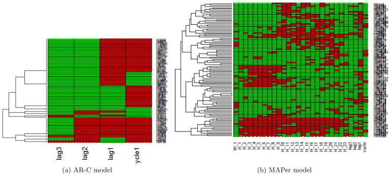
(a) AR-C model (b) MAPer model
Figure 3: Demonstrating how our modeling approach explains effect of different parameters using heatmap for randomly chosen 100 search log users. Each row represents a user and each column of a row represents the significance of a parameter for modeling the users behavior. Red (the darker shade) and green indicate significance and insignificance of corresponding parameters, respectively. Users who are similar in terms of their behavior model (i.e., set of learned parameters from training model), are clustered together.
Pearson Correlation Mean Square Error
Search log Twitter Search log Twitter
Personalized 0.337 0.491 0.041 0.045
Aggregated 0.127 0.192 0.114 0.064
Improvement 2.65 times 2.56 times 64% 30%
Table 5: Personalized models for each user significantly improve the prediction performance for both Twitter and search log datasets.
dataset. We found these interactive activities by adopting a frequent itemset mining approach (as described in Section 3.2). It indicates both residents 1 and 2 watch TV before going to sleep. Both of the residents are found to watch TV while having snacks. Resident 1 is found to talk on the phone before having lunch or dinner. These are also con-firmed in the actual dataset. Although resident 1 washes dishes often before / after breakfast and lunch, resident 2 washes dishes frequently after dinner and before going to bed. Hence, for resident 2 washing dishes influences sleep time. Due to space limitation, we are not showing the inter-active activities found in HOLMES dataset.
When we consider interaction among activities as features of prediction we find an increase in prediction performance of MAPer. The percent improvement of performance due to adding interaction is presented in Table 7. For exam-ple, in case of HOLMES dataset, the Pearson correlation of MAPer without interaction (Equation 5) and MAPer with interaction (Equation 4) are 0.385 and 0.583, respectively. So adding interaction features increases Pearson Correlation by 51% for HOLMES dataset.
6.2
Explanatory Power of MAPer
MAPer is an explanatory model as it uses the features that are relevant and specific to desirable human behavior.
Activity Influential Activities
R1:sleep brushing teeth, using internet, watching TV
R2:sleep brushing teeth, watching TV, washing dishes
R1:snack watching TV, using internet, talking on the phone R2:snack watching TV, having shower,
using internet
R1:breakfast preparing breakfast, using internet, watching TV
R1:lunch preparing lunch, talking on the phone, watching TV
R1:dinner talking on the phone, watching TV, preparing dinner
Table 6: Interaction among different activities of ARAS dataset: the left column contains the activities we want to predict and the right column contains the activities that in-teract with them.
Therefore each of the model parameters quantifies the effect of corresponding feature on the behavior. This is demon-strated in Figure 3 (a-b) using heatmap representation. Here we present two heatmaps of model parameters corre-sponding to the AR-C model and MAPer model for a set of randomly chosen 100 search log users. Figure 3 (a) demon-strates the lag and cycle features that are significant in the AR-C model for the 100 users. Figure 3 (b) demonstrates the lag, cycle, and multi-scale adaptive features that are sig-nificant in the MAPer model for the same set of users. Each row of a heatmap represents a user and each column of a row represent significance of a parameter (in terms of p-value) in the behavior model of that user. Here the red cells corre-spond to the significant parameters. Users who are similar in terms of their behavior model (i.e., set of learned parameters
Pearson Correlation Mean Square Error
ARAS HOLMES ARAS HOLMES
MAPer
w/o Interaction 0.7169 0.385 0.0184 0.0009
MAPer 0.782 0.583 0.016 0.0009
%Improvement 9 51 15
-Table 7: Increase in performance due to adding interaction features.
Parameter Range
Online Behavior Offline Behavior
Scale (hours) 1,2,4,6 1/2,1,2,4
Training set size (weeks) 2,4,6,8 NA6
Lag (hours) 2,3,4,6,8 1/2,1,2,3,4
Table 8: The range of different parameters used in experi-ments. The default values of parameters are shown in bold. from training model), are clustered together using hierar-chical agglomerative clustering algorithm. The explanatory power of MAPer is multi-fold.
Firstly, when comparing the two figures, we see that MAPer does not only capture the significance of lag and cycle, but also the significance of hour of the day and day of the week. This can serve as a useful behavior model for the end users. As MAPer not only predicts future behavior but also pro-vide a set of temporal contexts when the prediction accuracy of behavior is higher.
Secondly, from Figures 3a and 3b, MAPer has much higher number of clusters. Here a cluster represents a set of users who have similar model parameter and thus pre-sumably similar temporal behavior. So, MAPer essentially detects similar users in a more granular scale than the AR-C model. This is useful for detecting user community based on temporal behavior and finding an equivalent class of users.
Thirdly, unlike several existing methods MAPer directly quantifies the effect of a feature in behavior modeling. For instance, from Figure 3b, the feature corresponding to lag of order 3 is significant for only a handful of users. Thus we can infer which parameter is more important under dif-ferent temporal contexts for the behavior modeling of an individual.
6.3
Sensitivity Analysis
Here we evaluate our model by varying its hyper-parameters: temporal scale, training set size, and lag length (l). The de-fault value and range of each parameter are presented in Table 8.
6.3.1
Varying Training Set SizePearson Correlation Mean Square Error
Methods Search log Twitter Search log Twitter
2 weeks 0.4 0.52 0.039 0.044
4 weeks 0.34 0.49 0.041 0.045
6 weeks 0.31 0.45 0.042 0.048
8 weeks - 0.44 - 0.048
% Improvement 31 18 7 8
Table 9: Training set with more recent data results into better prediction.
In the previous sections we have used a dynamic training approach where for each data point in test set, we consider
6
As the sample size for most of the activities of both ADL dataset is too small to vary training period, this experiment was performed only on online behavior data
behavior data from the immediate previous 4 weeks as the training set. In this section we vary the training set size according to Table 9 and analyze its effect on prediction performance.
For search log data we vary training set size as 2, 4, and 6 weeks. For Twitter data, we vary training set size as 2, 4, 6, and 8 weeks. In both cases, smaller training set size results into smaller MSE and higher Pearson correlation. This indicates that human behavior changes over time and recent behavior is a better predictor of future behavior.
6.3.2
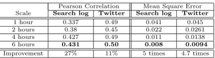
Varying Temporal ScalePearson Correlation Mean Square Error
Scale Search log Twitter Search log Twitter
1 hour 0.337 0.49 0.041 0.045
2 hours 0.38 0.45 0.022 0.0261
4 hours 0.427 0.49 0.011 0.0138
6 hours 0.431 0.50 0.008 0.0094
Improvement 27% 11% 5 times 4.7 times
Table 10: Varying temporal scale: larger scale results into better prediction performance for online behavior data.
So far, we have analyzed performance of different baseline methods and MAPer by keeping the temporal scale 1 hour for search log and Twitter data and half hour for ADL data. In this experiment we vary the temporal scale according to Table 8 and investigate its effect on prediction performance. We fix the other parameters in their default values.
For search log and Twitter data, higher temporal scale results into lower MSE and higher Pearson correlation (PC) (Table 10). Specifically, as we move from 1 hour to 6 hours’ scale, MSE decreases by about 5 times for both datasets. In terms of PC, with an increase in temporal scale there is 27% and 11% improvement in case of search log and Twitter data, respectively. This is because as we move to larger temporal scale the sparsity of data reduces and the task of parameter estimation gets less difficult.
On the other hand, in case of both of the ADL datasets the results vary with different scales without conforming to any particular trend. Because different temporal scales are suitable for modeling different activities. For example, while predicting sleep, half hourly scale results in better perfor-mance. But for predicting dinner, breakfast, and lunch, 2 hourly scale is more effective as the start time of these activ-ities slightly vary across different days. On average, there is 45% and 42% performance improvement due to scale varia-tion in terms of Pearson correlavaria-tion and mean square error, respectively. Due to space limit we are not tabulating the results from the two ADL datasets.
6.3.3
Varying Order of LagIn this experiment we vary the lag length as described in Table 8 while keeping the other parameters in their default values. The MSE values decrease very slightly with increase of lag for all four datasets. The Pearson correlation increases by 6.5%, 8.4%, 2% and 3% with increase of lag for search log, Twitter, ARAS, and HOLMES dataset, respectively. Over all the effect of changing lag is limited for all datasets. Due to space limitation, we are skipping the detailed results here.
7.
DISCUSSION
Our extensive experiments with four real world behav-ior data suggest that by using a combination of lag,
cy-cle, and interaction of activities, MAPer improves prediction performance significantly. They also demonstrate the effec-tiveness of using an adaptive learning approach that adapts with multi-scale temporal contexts. These features enable MAPer to perform equally or better than the parametric state-of-art SARIMA model. From an extensive sensitivity analysis, we discover that (i) using only 2 weeks data can result in higher accuracy for most of the online users, (ii) using recent training data is more useful as human behav-ior changes over time, and (iii) the suitable temporal scale vary over activities. In addition, MAPer yields explanatory results which can be useful for several interesting applica-tions. Such as, detecting user community or recommending friends based on similarity of temporal behavior as explained in Section 6.2. MAPer can be paired with text mining ap-proaches to provide personalized information retrieval, i.e., retrieving entertainment related queries during weekends. Other potential application domains where our model is ap-plicable include personalized human activity understanding, temporal user profiling, or social recommendations from an individual user’s online behavior.
We also find that MAPer is not generalizable to all human behavior as it assumes regularity in behavior. Hence, it’s performance is limited in case of predicting the need based behavior (e.g., issuing search query) or random behavior. In addition, using more granular temporal scales like minutes instead of hours can incur significant computational cost. Finally, evaluation using longer ADL datasets can yield more comprehensive results.
8.
CONCLUSION
With the surge of easy online access and ubiquitous sens-ing, abundant data contents have been generated that cap-ture the individual human behavior over time. In spite of having great potentials to provide real-time insights, per-sonalized temporal modeling of human behavior patterns remains largely unexplored. In this work, we introduce a multi-scale adaptive personalizedMAPermodel, an easy-to-interpret and simple-to-build predictive method for mod-eling the temporal dynamics of human behavior. Through results obtained from four real datasets of multiple individ-uals’ behavior records over time, our model yields statisti-cally significantly better predictions than a parametric state-of-art method (SARIMA model). Specifically, MAPer re-duces the mean square error of the SARIMA model by about 15%, 31%, and 10% for the Twitter, ARAS, and HOLMES datasets, respectively.
Currently we are using only temporal footprint of activi-ties. In the future, we want to model behavior by extracting textual features from user generated contents. We also want to combine virtual and physical world behaviors of an indi-vidual using smart devices.
9.
ACKNOWLEDGMENTS
This paper was supported, in part, by NSF grant CNS-1319302.
10.
REFERENCES
[1] F. Abel, Q. Gao, G.-J. Houben, and K. Tao. Analyzing user modeling on twitter for personalized news recommendations. In User Modeling, Adaption and Personalization, pages 1–12. Springer, 2011.
[2] E. Adar, D. S. Weld, B. N. Bershad, and S. S. Gribble. Why we
search: visualizing and predicting user behavior. InProceedings
of the 16th international conference on World Wide Web (WWW), pages 161–170. ACM, 2007.
[3] H. Alerndar, H. Ertan, O. D. Incel, and C. Ersoy. Aras human activity datasets in multiple homes with multiple residents. In IEEE PervasiveHealth, 2013.
[4] F. Baskaya, H. Keskustalo, and K. J¨arvelin. Modeling
behavioral factors ininteractive information retrieval. In Proceedings of the 22nd ACM international conference on information & knowledge management (CIKM), pages 2297–2302. ACM, 2013.
[5] C. Borgelt. Frequent item set mining.Wiley Interdisciplinary
Reviews: Data Mining and Knowledge Discovery, 2(6):437–456, 2012.
[6] Y. Chen, D. Pavlov, and J. F. Canny. Large-scale behavioral
targeting. InACM SIGKDD, 2009.
[7] Z. Cheng, J. Caverlee, and K. Lee. You are where you tweet: a
content-based approach to geo-locating twitter users. InACM
SIGKDD, 2010.
[8] M. Clements and D. Hendry.Forecasting economic time series.
Cambridge University Press, 1998.
[9] J. F. Desforges, W. B. Applegate, J. P. Blass, and T. F. Williams. Instruments for the functional assessment of older
patients.New England Journal of Medicine,
322(17):1207–1214, 1990.
[10] H. Gao, J. Tang, X. Hu, and H. Liu. Modeling temporal effects of human mobile behavior on location-based social networks. In ACM CIKM, 2013.
[11] S. A. Golder, D. M. Wilkinson, and B. A. Huberman. Rhythms of social interaction: Messaging within a massive online
network. InCommunities and Technologies 2007, pages 41–66.
Springer, 2007.
[12] J. D. Hamilton.Time series analysis, volume 2. Princeton
university press Princeton, 1994.
[13] E. Hoque, R. F. Dickerson, S. M. Preum, M. Hanson, A. Barth, and J. A. Stankovic. Holmes: A comprehensive anomaly
detection system for daily in-home activities. InProceedings of
the 11th IEEE international conference on distributed computing in sensor systems, 2015.
[14] R. J. Hyndman, Y. Khandakar, et al. Automatic time series for forecasting: the forecast package for r. Technical report, Monash University, Department of Econometrics and Business Statistics, 2007.
[15] M. G. Kendall and J. K. Ord.Time-series, volume 296.
Edward Arnold London, 1990.
[16] J. R. Kwapisz, G. M. Weiss, and S. A. Moore. Activity
recognition using cell phone accelerometers.ACM SigKDD
Explorations Newsletter, 12(2):74–82, 2011.
[17] J. Liu, Y. Liu, M. Zhang, and S. Ma. How do users grow up along with search engines?: a study of long-term users’
behavior. InACM CIKM, 2013.
[18] H. L¨utkepohl.Vector autoregressive models. Springer, 2011.
[19] M. Naaman, A. X. Zhang, S. Brody, and G. Lotan. On the
study of diurnal urban routines on twitter. InICWSM, 2012.
[20] E. Nazerfard and D. J. Cook. Using bayesian networks for daily
activity prediction. InAAAI Workshop: Plan, Activity, and
Intent Recognition, 2013.
[21] G. Pass, A. Chowdhury, and C. Torgeson. A picture of search. InInfoScale, volume 152, page 1. Citeseer, 2006.
[22] K. Radinsky, K. Svore, S. Dumais, J. Teevan, A. Bocharov, and E. Horvitz. Modeling and predicting behavioral dynamics on
the web. InACM WWW, 2012.
[23] J. Scott, A. Bernheim Brush, J. Krumm, B. Meyers, M. Hazas, S. Hodges, and N. Villar. Preheat: controlling home heating
using occupancy prediction. InProceedings of the 13th
international conference on Ubiquitous computing, pages 281–290. ACM, 2011.
[24] P. V. Senin. Literature review on time series indexing. 2009. [25] W. Weerkamp and M. De Rijke. Activity prediction: A
twitter-based exploration. InSIGIR Workshop on Time-aware
Information Access, 2012.
[26] M. Ylvisaker and T. J. Feeney.Collaborative brain injury
intervention: Positive everyday routines.Singular Publishing Group, 1998.
[27] Y. Zhu, E. Zhong, S. J. Pan, X. Wang, M. Zhou, and Q. Yang.
Predicting user activity level in social networks. InACM