A persistent incremental learning approach for object classification of unseen categories using convolutional neural networks on mobile robots

Freigabe: Der Bearbeiter: Unterschriften Markus Knauer

Betreuer:

Maximillian Denninger Der Institutsdirektor Prof. Alin Albu-Schäffer

Dieser Bericht enthält 120 Seiten, 50 Abbildungen und 33 Tabellen

Institut für Robotik und Mechatronik

BJ.: 2020

IB.Nr.: DLR-IB-RM-OP-2020-115

MASTERARBEIT

A PERSISTENT INCREMENTAL

LEARNING APPROACH FOR OBJECT

CLASSIFICATION OF UNSEEN

CATEGORIES USING CONVOLUTIONAL

NEURAL NETWORKS ON MOBILE

ROBOTS

Studiengang Informatik Master of Science

A Persistent Incremental Learning Approach for

Object Classification of Unseen Categories using

Convolutional Neural Networks on Mobile Robots

Markus Knauer Matrikelnummer

305721

Aufgabensteller/Pr¨ufer Prof. Dr. J¨urgen Brauer Zweitkorrektor Prof. Dr. Jochen Staudacher Arbeit vorgelegt am 28.08.2020

durchgef¨uhrt in der Fakult¨at Informatik

durchgef¨uhrt bei Deutsches Zentrum f¨ur Luft- und

Raumfahrt e. V. (DLR), Oberfaffenhofen, Institut f¨ur Robotik und Mechatronik, Perzeption und Kognition (RM/PEK-OP)

Betreuer Maximilian Denninger, RM/PEK-OP

PD Dr. Rudolph Triebel, RM/PEK-OP Leitung Anschrift des Verfassers Romatsrieder Straße 27, 87654 Friesenried

I

Abstract - German

Die Verwendung von neuronalen Netzen, insbesondere von Convolutional Neural Networks (CNN), hat in vielen Bereichen, wie etwa der Objekt-Klassifikation, zu guten Ergebnissen gef¨uhrt. Diese Netze sind jedoch dadurch limitiert, dass sie nur einmal trainiert und an-schließend f¨ur die Auswertung von ¨ahnlichen Daten eingesetzt werden. Es k¨onnen also nur diejenigen Aufgaben durchgef¨uhrt werden, welche zu Beginn gelernt wurden. Kommen nun neue Aufgaben hinzu, muss das Netzwerk nochmals mit allen Daten neu trainiert werden. Diese Netze sind daher normalerweise nicht in der Lage, kontinuierlich hinzuler-nen zu k¨onnen. In dieser Arbeit wird ein neuer Ansatz vorgestellt, welcher in der Lage ist fortlaufend neue, bisher unbekannte Objekt-Kategorien auf Bildern hinzulernen zu k¨onnen. Das Ziel hierbei ist eine Anwendung im Bereich der mobilen Robotik. Zun¨achst werden hierzu verschiedene Strategien vorgestellt, welche die Architektur des Netzwerks dynamisch erweitern, sobald neue Kategorien hinzugelernt werden sollen. Im ersten Ansatz wird die letzte Neuronenschicht des Netzwerkes dynamisch an die Anzahl der Kategorien angepasst. Der zweite Ansatz erweitert diese Technik, indem f¨ur jede Sequenz von neuen Kategorien zus¨atzliche Neuronenschichten angelegt werden. Um zu verhindern, dass das Netzwerk bisher Erlerntes wieder vergisst, werden zus¨atzlich verschiedene Reg-ularisierungsstrategien vorgestellt. Unter anderem auch eine neue Methode, bei welchem der Classification-Loss durch einen Regression-Loss ersetzt wird. F¨ur das Problem einer Ungleichverteilung der Output-Werte, wird ein neuartiger Ansatz vorgestellt, bei dem die Output-Werte durch die Varianz der jeweiligen Kategorie geteilt, und somit ausgeglichen werden. Zu dieser Arbeit geh¨ort auch ein neuer Datensatz f¨ur Continual Learning, welcher speziell f¨ur die Service-Robotik entwickelt wurde (HOWS-CL-25). Dieser besteht aus 150.795 synthetischen Farbbildern von 25 verschiedenen Haushaltsobjektkategorien. Der hier vorgestellte Ansatz wird in den Bereich des Online Learnings eingeordnet. Dies ist eine spezielle Art des Incremental Learnings, bei welchem das Netzwerk lediglich Zugriff auf die Trainingsbilder der aktuellen Sequenz hat und vorherige Trainingsbilder nicht gespeichert werden d¨urfen. Diese Methode wird auch als Rehearsal-free bezeichnet. On-line Learning ist ein noch ungel¨ostes Problem und komplexer, als andere inkrementelle Ans¨atze, welche Zugriff auf alte Trainingsbilder haben. Der Ansatz dieser Arbeit wurde auf verschiedenen Datens¨atzen evaluiert und mit anderen Ans¨atzen aus der Literatur ver-glichen. Dies beinhaltet auch eine Evaluation auf dem CLVISION Workshop der CVPR 2020.

Abstract

Neural Networks and especially Convolutional Neural Networks (CNN) show remarkable results in many fields, among others in object classification and recognition. But these networks are limited by the tasks they are trained on, as they are designed to learn all tasks they will need during their lifetime in the beginning and hence are frozen. If now new tasks arrive, the network has to be trained completely new. These networks are therefore usually not able to learn in a continual manner, like humans are capable of. In this work, a novel approach is presented, where a deep neural network is used to contin-ually learn new unseen object categories on images, which can be used in different fields, like mobile robots. First, different architectural strategies are proposed to dynamically adapt the network according to the categories it learns over time. This includes one strategy, where the last layer of our network is adapted and another one where multiple fully-connected layers are created for each new sequence. In order to prevent forgetting, different regularization strategies are shown, including a novel loss function where the classification is replaced by a regression. So, it is ensured that already learned categories are not forgotten by simultaneously enabling the network to learn new categories. Fur-thermore, the emerging problem of a discrepancy in the output distribution is recognized and different solutions are proposed. This includes a novel regularization strategy, where the outputs are divided by the variance per category. Finally, a novel dataset for contin-ual learning is presented, which is especially suited for object recognition in our mobile robot environment (HOWS-CL-25). It consists of 150,795 synthetic images of 25 different household object categories in a randomly changing environment. Our approach can be classified as online learning, a special variant of incremental learning, where one is lim-ited by the data the network can observe in a specific time step, without the access to previous training examples - also called rehearsal-free. This is a challenging and unsolved problem in comparison to other incremental learning approaches, which also use previous training examples, but as this thesis is focusing on an approach for mobile robots, online learning is more relevant. Our approach is tested on different datasets and compared with other solutions from literature. Additionally, our method was evaluated in the CLVISION workshop at CVPR 2020.

III

Acknowledgements

I would like to thank my supervisor Maximilian Denninger, as well as the rest of my team at DLR, who helped me through my whole master thesis. Additionally, I would like to thank Dr. Rudolph Triebel, who made it possible for me to research in such an exciting field at an outstanding research institute. I had the chance to deepen my knowledge within a high class research environment, at workhops and hackatons, especially in the field of Computer Vision, Deep Learning and Continual Learning, which I will benefit greatly from. I would also like to thank my professor Prof. Dr. J¨urgen Brauer and his PhD. Student Bonifaz Stuhr for all the good advises in an open and friendly environment. Thanks to all of them, I had a great environment to write my masters thesis, where I also had a lot of fun, researching on Continual Learning.

Contents

Abstract German I

Abstract English II

Acknowledgements III

List of figures VII

List of tables IX

Table of abbreviations XII

1 Motivation 1

2 Introduction 3

2.1 Problem description . . . 4

2.1.1 Catastrophic forgetting . . . 4

2.1.2 Aim of this thesis . . . 6

2.2 Incremental Learning procedure . . . 6

2.3 Thesis structure . . . 7

3 Related work 8 3.1 Definition and differentiation . . . 8

3.2 Continual Learning strategies . . . 10

3.3 Progressive Neural Networks (PNN) . . . 11

3.4 Copy Weight with Reinit (CWR) . . . 12

3.5 Learning without forgetting (LWF) . . . 13

3.6 Elastic Weight Consolidation (EWC) . . . 14

3.7 Synaptic Intelligence (SI) . . . 15

3.8 Incremental Classifier and Representation Learning (iCaRL) . . . 15

3.9 Gradient Episodic Memory (GEM) . . . 16

3.10 Continuous Learning in Single-Incremental-Task Scenarios (AR1) . . . 18

3.11 Persistent Anytime Learning of Objects from Unseen Classes (PAL) . . . . 19

4 General 21 4.1 Activation functions . . . 21

4.2 Convolutional Neural Networks . . . 23

Contents V

4.2.2 Inception-v3 . . . 28

4.2.3 InceptionResNet . . . 30

4.3 Our baseline approach . . . 30

5 Our Approach 32 5.1 Architectural strategies . . . 32 5.1.1 Expanding Network . . . 32 5.1.2 Different Heads . . . 33 5.2 Regularization Strategies . . . 37 5.2.1 Reconstruction label . . . 37 5.2.2 Loss function . . . 41

5.2.3 Discrepancy in output distribution . . . 44

5.2.4 Reconstruction loss . . . 47 5.2.5 Further techniques . . . 49 6 Experimental setup 51 6.1 Environment . . . 51 6.2 Datasets . . . 51 6.2.1 COIL-100 . . . 53 6.2.2 CORe50 . . . 54

6.2.3 Creation of a new dataset . . . 57

6.3 Training- and validation procedure . . . 62

6.3.1 Training procedure . . . 62

6.3.2 Validation and testing procedure . . . 62

6.4 Implementation details . . . 63

6.4.1 Feature extraction networks . . . 67

7 Results 68 7.1 CORe50 . . . 68

7.1.1 Confusion matrix on CORe50 . . . 71

7.1.2 CLVISION Challenge at CVPR2020 . . . 71 7.1.3 CORe50 leader-board . . . 73 7.2 Our Dataset . . . 74 8 Ablation studies 79 8.1 Batch normalization . . . 79 8.2 Activation Function . . . 81 8.3 Initialization . . . 82

8.4 Feature extraction networks . . . 82

8.5 Freezing or fine tuning . . . 82

8.6 Number of layers . . . 83 8.7 K-nearest neighbor . . . 84 9 Future steps 85 9.1 Rehearsal Strategy . . . 85 9.2 Dreaming . . . 85 9.3 Uncertainty Estimation . . . 87 9.4 Active Learning . . . 88 9.5 Inverted GLOs . . . 88 10 Conclusion 91 References 93 11 Appendix 102 11.1 Appendix A: Parameter of the best result on the CORe50 dataset . . . 102

11.2 Appendix B: Parameter of the best result on the HOWS-CL-25 dataset . . 103

List of figures VII

List of figures

1.1 Continual learning example on our robot Justin . . . 1

2.1 Example for comparable features . . . 5

2.2 The incremental learning procedure . . . 7

3.1 Definition of online-, incremental- and continual learning . . . 8

3.2 Venn diagramm of incremental learning strategies . . . 11

3.3 Comparison of EWC, iCaRL and GEM . . . 17

3.4 Persistent anytime learning . . . 20

4.1 Identity activation function . . . 21

4.2 RELU activation function . . . 21

4.3 ELU activation function . . . 22

4.4 SELU activation function . . . 22

4.5 CRELU activation function . . . 22

4.6 SIREN activation function . . . 23

4.7 Visualization of the ResNet50 architecture . . . 25

4.8 Comparison of the two types of ResNet blocks . . . 26

4.9 Comparison of skip connections in deep neural networks . . . 26

4.10 Architecture of the different ResNet versions . . . 27

4.11 Inception module . . . 28

4.12 Inception module with dimensional reduction . . . 29

4.13 Inception-v3 architecture . . . 29

4.14 An example part of the InceptionResNet . . . 30

4.15 Our baseline-network architecture . . . 31

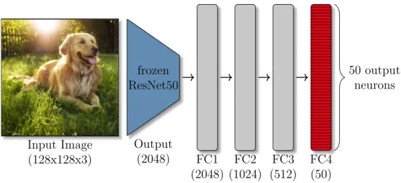
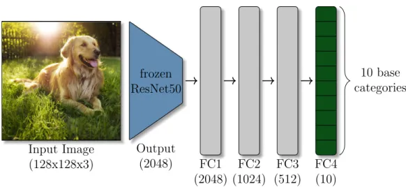
5.1 Base Training . . . 33

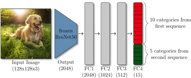
5.2 Expanding network at the second sequence . . . 34

5.3 Expanding network in sequence eight . . . 34

5.4 The network expanding its heads . . . 36

5.5 Calculation of the reconstruction label . . . 40

5.6 Three-part loss function . . . 43

5.7 Distribution discrepancy at learned neurons . . . 44

5.8 Variance per category . . . 45

5.9 Distribution discrepancy at the new neurons . . . 46

5.10 Normalization solution for distribution discrepancy . . . 47

6.1 Example pictures of the COIL-100 dataset . . . 53

6.2 Example pictures of the CORe50 dataset . . . 54

6.4 Overview of the HOWS-CL-25 dataset . . . 59

6.5 Example for the different image types of the HOWS-CL-25 dataset . . . . 60

6.6 An example of our scatter plot evaluation . . . 65

6.7 A TensorBoard example run . . . 66

7.1 Accuracy on the CORe50 dataset . . . 70

7.2 The performance of our approach over the sequences on CORe50 . . . 71

7.3 Confusion matrix on the CORe50 dataset . . . 72

7.4 Image examples of the fourth sequence of the HOWS-CL-25 dataset . . . . 76

7.5 Accuracy on HOWS-CL-25 . . . 76

7.6 The performance of our approach over the sequences of HOWS-CL-25 . . . 77

8.1 Batch Normalization . . . 80

9.1 Incremental learning via memory replay . . . 86

9.2 Uncertainty estimation network . . . 87

9.3 Active learning network . . . 88

List of tables IX

List of tables

3.1 Online and incremental learning . . . 9

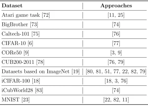
6.1 Variety of datasets used for continual learning . . . 51

6.2 Categories of sequence 0 . . . 59

6.3 Categories of sequence 1 . . . 59

6.4 Categories of sequence 2 . . . 60

6.5 Categories of sequence 3 . . . 60

6.6 Categories of sequence 4 . . . 60

6.7 Online and incremental learning . . . 61

6.8 Requirements fulfillment of HOWS-CL-25 . . . 61

6.9 Our shuffle- and batch-size settings . . . 64

6.10 Implementation characteristics of the different feature extraction networks 67 7.1 Offline results of the different sequences of CORe50 . . . 68

7.2 Baseline approach on CORe50 . . . 69

7.3 Modified baseline approach on CORe50 . . . 69

7.4 Results of our approach on CORe50 . . . 70

7.5 Extraction of CLVISION challenge results for scenario NC . . . 73

7.6 Extraction of CLVISION challenge results for scenario NI . . . 73

7.7 CORe50 leader-board . . . 74

7.8 Offline results of the different sequences of the HOWS-CL-25 . . . 74

7.9 Results of our baseline approach on HOWS-CL-25 . . . 75

7.10 Results of our modified baseline approach on HOWS-CL-25 . . . 75

7.11 Results of our approach on HOWS-CL-25 . . . 75

7.12 Impact of our proposed techniques . . . 78

8.1 Results on CORe50 and HOWS-CL-25 for different placed batch norms . . 80

8.2 Results on CORe50 and HOWS-CL-25 for different activation functions . . 81

8.3 Results on CORe50 and HOWS-CL-25 for different initialization strategies 82 8.4 Results of different feature extraction networks . . . 83

8.5 Results of different freezing strategies on CORe50 . . . 83

8.6 Results of different amounts of fully-connected layers . . . 84

11.1 Parameter of the best CORe50 result of our approach . . . 102

11.2 Parameter of the best HOWS-CL-25 result of our approach . . . 103

11.3 Hyperparameter part 1 . . . 104

Table of Abbreviations

ADAM Adaptive moment estimation - optimizer [1]

AlexNet CNN architecture [2]

AR1 Continal learning strategy, which combines architectural and regularization techniques [3]

BlenderProc A procedural Blender pipeline for photorealistic training image generation [4, 5]

CIFAR-100 Canadian Institute For Advanced Research dataset [6]

CL Continual Learning

CLVISION Continual Learning on computer vision, workshop at CVPR 2020 [7]

CNN Convolutional Neural Network

COIL-100 Columbia Object Image Library [8]

CORe50 A dataset and benchmark for Continual Learning, Object Recognition, Detection and Segmentation [9]

CRELU Concatenated Rectified Linear Unit - activation function [10] CVPR IEEE Conference on Computer Vision and Pattern Recognition CWR Copy weights with re-init [9]

CWR+ extended, improved CWR [3]

DLR Deutsches Zentrum f¨ur Luft- und Raumfahrt e.V. EWC Elastic Weight Consolidation [11]

ELU Exponential Linear Unit - activation function [12] GAN Generative Adversarial Network [13]

GEM Gradient Episodic Memory [14] GLO Generative Latent Optimization [15]

Abk¨urzungsverzeichnis XI

GoogLeNet CNN architecture [17]

HOWS-CL-25 Household Objects Within Simulation dataset for Continual Learning (ours)

iCaRL Incremental Classifier and Representation Learning [18] iCIFAR-100 Modified CIFAR-100 dataset to be incremental [18] ImageNet One of the biggest public image databases [19] Inception-v3 CNN architecture [20]

InceptionResNet CNN architecture [21]

KNN K-nearest neighbor

LWF Learning Without Forgetting [22] MNIST database of handwritten digits [23]

NC Multi-task new classes scenario of CORe50 dataset NI New Instances scenario of CORe50 dataset

OP Company location Oberpfaffenhofen PAL Persistent Anytime Learning [24]

PEK Department for Perception und Cognition PNN Progressive Neural Network [25]

RELU Rectified Linear Unit - activation function [26] ResNet50 CNN architecture [27]

ResNet50V2 Second version of ResNet50 - CNN architecture [28] RM Institut of Robotics und Mechatronics

SELU Scaled Exponential Linear Units - activation function [29] SGD Stochastic gradient descent - optimizer [30]

SIREN Implicit Neural Representations with Periodic - activation functions [32]

TFRecord Data-format from tensorflow, which is optimized for streaming data over a network

1 Motivation 1

1 Motivation

In the past decade, the demand for social caregivers has risen drastically, especially in countries like Germany or Japan, where an ageing society is already at an advanced stage. This has lead to a reinforced research pull in the field of service robotics. Robots are already in use to assist the human work in industry or in places where it is too dangerous for humans, like in outer space. Therefore, robots showed to be predestined for assisting humans. In social care, they could help elderly care takers to grasp objects, open doors, getting out of bed, alarm others in a case of danger or accident and much more. These robots need an elaborate understanding of their environment including the capabilities to learn new things on the fly. As humans have this skill since birth, it is hard for them to comprehend the limitations of robots, which usually can only learn once and are henceforth unable to learn new things.

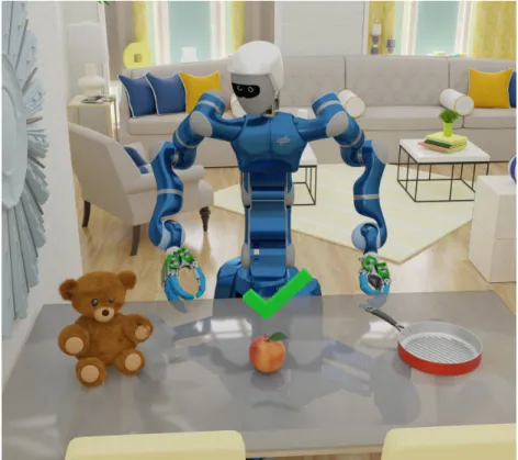
For a better understanding figure (1.1) is provided, where Justin, a service robot from the DLR is shown. There he finds three new objects, he has never seen before. As a service robot, he is operating in a constantly changing environment. So Justin should be

Figure 1.1: Continual learning example on our robot Justin: As a service robot, Justin is working in a constantly changing environment. On this picture he found three new objects he has never seen before. This thesis is motivated to solve the problem allowing Justin to learn new object categories on the fly without forgetting already learned ones.

able to learn these objects, even if he was not trained on them before. This thesis tries to tackle this problem of continual learning, where new things are introduced during the lifetime of our robotic system.

In the field of incremental learning, the thesis introduces a novel online learning ap-proach, to be able to learn new object categories, when the need arises. In order to get closer to a future, where mobile robots can be deployed in everyday homes help and serve our caregivers.

The ability to continually learn new tasks, in our case object categories, therefore is highly rewarding. Incremental learning can be used in other fields, too. Robots in industrial production are used for welding, grapping, lifting, etc. Those robots are able to only fulfill one task, they are programmed for. As soon as one of the component characteristics, like the material or the size changes, the robot is not able to carry out the work step anymore, without being completely reprogrammed. Our approach could be used there to learn those new categories, so that the robot knows what it’s dealing with. A robot which is able to dynamically adapt to new conditions, by only learning new tasks while still be able to conduct the old tasks, would save a lot of money by reducing machine downtime.

Our approach can be used outside of the field of robotic as well. For example, at online retailers like Amazon, for continually identification and classification of uploaded product pictures.

2 Introduction 3

2 Introduction

”The transfer of knowledge within the lifetime of an individual has been found to be one of the dominating factors of natural learning and intelligence. If computers ever are to exhibit rapid learning capabilities similar to that of humans, they will most likely have to follow the same

principles.” Sebastian Thrun (1996 [34] page 193).

Humans are remarkably good in absorbing new knowledge about unknown things very fast from only a few single examples, continually throughout their lifetime. Thus, life-long learning presents a crucial capability in our daily life. Deep neural networks have shown excelled results on a wide range of problems, from recognition, reconstruction and localization tasks in computer vision, language processing, etc. [27, 35, 36, 37]. Typically, these algorithms apply batch-wise training to large datasets e.g. ImageNet [19] and need many iterations of the whole dataset to obtain satisfactory performance. In contrast to humans, neural networks rely on a training with the whole, static dataset, containing everything they have to know. This dataset is then repetitively presented to the network to obtain a good generalization and accuracy. Usually, this presenting has to be done several thousand times. That means, everything the network should learn has to be avail-able before the training starts. Continually learning new tasks through the lifetime of a neural network is therefore not possible. If new things arrive, which the network is not able to compensate by generalization, the network has to be trained completely again, as generalization is limited to known categories. In this thesis a novel algorithm, to solve this problem, is presented and different solution strategies are evaluated. With our approach, the robot is enabled to learn new things on the fly, without the need of retraining the whole network. In contrast to most of other solutions in literature, this approach does not use additional memory to store previous training data.

Our aim is to solve the problem of continually learning new object categories, in a setting with a limited memory capacity, where it is not possible to save data from previously learned categories, like images. This so called online learning strategy is more difficult, but also more practically relevant for service robots, as those are limited on disc space and sometimes, it is not possible to save images of each category, the robot knows so far. Thus solving this problem without the need of previous training data would be the faster, saver and less storage intensive solution. Therefore, the focus of this thesis is on online learning. Additionally, a possible integration of the so called rehearsal strategy is shown at the end of the work, where it is allowed to reuse previous training data.

continual manner. Those problems are described in the next section.

2.1 Problem description

Taken an theoretically infinite stream of data, a continual learning algorithm has to learn from a sequence of data or data-batches, without access to the whole dataset. Commonly used neural networks for object classification, like ResNet50 or Inception-v3, are not designed to be used in a continual learning process, as their main focus is on learning only once. This is due to the fact that these more researched, non-continual learning algorithms have access to all the data in the beginning. If those are used to train in a continual manner, the network suffers from forgetting [38]. In the following, this problem is described in more detail and the aim of this thesis is defined.

2.1.1 Catastrophic forgetting

Forgetting is one of the biggest problems continual learning algorithms face nowadays. It describes the problem, when a network forgets previously gathered knowledge by learning new tasks. In literature, this is known as catastrophic forgetting or catastrophic inference [38, 39]. This problem applies in particular for networks, which use a softmax and cross-entropy as classification loss. There, the network experiences a rapid overwriting of the model parameters, when learning in a continual manner [40]. These methods are state-of-the-art in the field of classification in computer vision, but are not suited for continual learning.

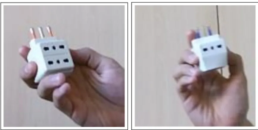
The reason of catastrophic forgetting, in the context of continual learning, is the lack of comparable features between the categories of the different sequences. A good example is the way a human would learn different categories. For example: Assuming, there is a human subject, who doesn’t know the categories ”dog” and ”cat” (see figure 2.1). There are now two possible ways to teach this. First, by showing a lot of different dog pictures. Thereby, our subject might discover that a dog has four paws, two eyes and a snout. But after the person also observes some cat pictures, the emerging problem of this procedure is shown, as the subject will not be able to see a difference between dogs and cats, as they are having a lot of features in common. Another, more effective way, is by showing the person pictures of dogs and cats simultaneously. By finding the difference between both categories, our subject will be able to recognize dogs and cats after the training. The same problem occurs for neural networks. As the training examples of previous categories are not longer available, the network can not find the differences to the current shown categories. Therefore, it is not able to learn new categories, without forgetting the old ones.

2 Introduction 5

Figure 2.1: Example for comparable features: A dog and cat are shown to a human, who does not know either. If the subject first observes the dog- and later the cat images it is much more difficult to learn how to distinguish between those two categories, then by showing images of dogs and cats simultaneously. The pictures are from [41] and [42].

An example of catastrophic forgetting is shown in table 7.2 of our result section. The challenge now is to find a way to prevent this catastrophic forgetting.

Data distribution shift Another reason for forgetting can be found in literature, which is named data distribution shift [43, 44]. Gepperth et al. and Lesort et al. found, that taking temporal structure of data samples into account, one can observe changes in the data distribution that occur over time. This also applies to continual learning, as there a form of temporal structure is used. This refers to the fact, that the different tasks are split into several sequences, which are learned chronologically by the network (see 2.2). Those changes in data statistics are referred to as concept drift orconcept shift [43]. Especially online learning suffers from this problem, as it does not keep data of previous examples, to compare the new data with. If there is no external information about a data distribution shift, the continual learning algorithm has to detect it. Otherwise an undetected shift would lead to forgetting [44].

According to Gepperth et al. [43], concept drifts can be distinguished in two different types:

• Virtual concept driftorcovariate shiftoccur by changes in the input distribu-tion, which can easily appear, e.g., due to adding of dissimilar object categories to a classification problem causing an imbalance distribution.

• Real concept driftis caused by novelty on data or new categories, e.g., when the model has to be re-adapted on visually similar, but new categories, which is at the core of continual learning.

These concept drifts can happen gradually or abruptly and may also appear when changing the task of the network.

Knowledge transfer In order to deal with catastrophic forgetting, one has to find a strategy to handle the knowledge within the network. In continual learning, there are a lot of different ways to store information about already learned tasks:

• Raw data from image examples

• Any kind of representation of the training examples, e. g. latent space • Model weights

• Regularization matrices, e.g. importance matrix • Reconstruction values, etc.

An efficient strategy should be able to only save important data and transfer this knowl-edge through all sequences, to mitigate forgetting. A combination of these strategies is common as described in chapter 3.2. Further information of the different techniques are described in our related work section 3.

2.1.2 Aim of this thesis

The aim of this thesis is to develop an approach, which is able to learn unkown object categories on continually appearing images, in a robotic environment, considering the problems, described before. The solution should be applied in the field of computer vision, by using a convolutional neural network. Furthermore, approaches are preferred, where additional memory for old training examples is not necessary (online learning).

2.2 Incremental Learning procedure

In order to simulate a continuous learning process, the training and validation procedure has to be adapted accordingly. Usually, a neural network learns all training examples at once. But in the case of incremental learning, the network starts with a basic knowledge and then continually learns new tasks over time. As shown in figure 2.2 the incremental learning procedure is conducted differently to the standard way, a neural network is trained. Here, the training images arrive in batches, distributed over sequences and each category is only available in one sequence. For example, the first sequence contains categories [0−9], the second sequence categories [10−14], etc. Thus, category ”apple” is only available in sequence zero and nowhere else. This comes close to a practical situation,

2 Introduction 7 t Sequence 0 (base) category 0 - 9 Sequence 1 category 10 - 14 . . . Sequence n

Figure 2.2: The incremental learning procedure: The different object categories are di-vided into sequences, which are shown to the network over time. Each cate-gory is only available in one of those sequences and the network therefore only has access to the images of the certain categories during this sequence. In the next sequences, the task is to learn new categories, while not forgetting the old ones. This graphic uses pictures from the HOWS-CL-25 dataset.

when a robot observes new, unseen objects, as shown in figure 1.1. Continually learning new objects it observes over time, is much more challenging, than training with the images of all categories at once, since the network must always keep the knowledge from previous sequences.

2.3 Thesis structure

After the introduction into the topic of this thesis and a problem description, an evaluation of solutions from literature and their difference to our approach are discussed in the related work chapter. After that, important methods of our work are described more detail in the chapter ”General”. Then, our approach is presented in the following chapter. The used datasets, as well as details to the learning procedure and implementation are shown in an experimental setup, followed by the achieved results. In our ablation studies, the impact of different hyperparameter choices are presented. In the end of this thesis, future steps are discussed, followed by a conclusion. Additional information on the used hyperparameters are attached in the appendix.

3 Related work

In this section, the definition of continual learning and its solutions from literature are discussed. This includes their advantages and disadvantages and a highlighting of their differences to our approach. After an overview, where the different methods are subdivide into three strategies, the approaches are discussed in more detail.

3.1 Definition and differentiation

In literature, there are several definitions of the process, of continually learning new things, like categories, instances or tasks. Gepperth and Hammer [43] or Rebuffi et al. [18] call itIncremental Learning, Chen and Liu [45] or Thrun and Mitchell [46] Lifelong Learning

and Carlson et al. [47] and Mitchell et al. [48] call it Never Ending Learning. Like Lesort et al. [44], this thesis refers to all continuous, incremental and lifelong learning synonyms as continual learning (CL). In our definition, incremental learning is a sub-area of continual learning, where new tasks are learned chronological over time. And online learning, on the other hand, is defined as a sub-area of incremental learning, where the network only has access to the current task and explicitly not to previous tasks (see figure 3.1). The difference between those three areas is shown in table 3.1. Online learning is the most challenging part of incremental learning and the major focus of this thesis.

Continual Learning

Incremental Learning

Online Learning

Figure 3.1: Definition of online-, incremental- and continual learning: In general, the pro-cedure of continually learning new tasks is known in literature as continual learning. Incremental learning is defined as a part of continual learning, which deals with sequentially appearing data, thus new tasks are learned chronolog-ical over time. Online learning is a special kind of incremental learning, where the network only has access to the current task.

3 Related work 9

Table 3.1: Online and incremental learning

Research area Description

Continual Learning All different techniques to continually learn new tasks.

Incremental Learning Sequential continual learning, where data arrives in chronological batches.

Online Learning Special case of incremental learning, where data of previous sequences are not avail-able. Also called rehearsal-free incremen-tal learning.

The research field of continual learning is interlocked with many other areas and works, which are often used in combination, in order to improve or to build a base for another technique.

A lot of continual learning algorithms are based ontransfer learning [49, 50, 51, 52], where knowledge is gathered from previously learned tasks. A common way is e.g. to pretrain the network on ImageNet [19] and then fine tune it on example images of the categories, the network actually should learn. Compared to continual learning, the net-work does not have to be able to solve previously learned tasks. Therefore, this approach cannot be adapted on a one-to-one basis. In computer vision, this is also referred as

domain adaption [53].

A similar approach is meta learning [54, 55], a sub-field of machine learning, where metadata about previously gathered knowledge is used as a hyper parameter. The goal is, to use this metadata to understand how different algorithms perform on a given tasks and therefore improve the performance of an existing learning algorithm, or to learn the algorithm itself. It is also known as ”learning to learn”. As well as transfer learning, also a modified meta learning approach could be used for continual learning.

Especially in the field of robotics few-shot learning [56] becomes interesting. It describes the ability to learn tasks from only a few examples, as taking training examples is very time-consuming. If the robot only needs to take a few images, the whole process would greatly benefit. This method has nothing to do with continual learning directly, but could be used as a further improvement step for an already created approach.

As neural networks tend to be overconfident, the research field of uncertainty esti-mation becomes important for continual learning [57]. It contains methods to measure the certainty of the network about its own prediction, which becomes crucial, especially for service robots, as wrong classifications would hurt the trust of the user.

where, for example, the system interactively asks the user for the label of a new, unknown object category, which it detects itself. Here, it is important to know, what the robot does not know, to trigger a further handling on those examples.

3.2 Continual Learning strategies

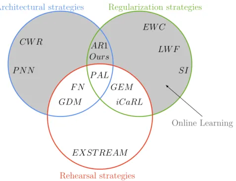
The field of continual learning (CL) can be divided into three strategies, as shown in figure 3.2 [3]. After this short overview, each method will be described more deeply.

• Architectural strategies: These are strategies, which try to moderate forgetting by changing the architecture of the neural network. For instance, by using special architectures, layer changing or different freezing strategies. Here, these changes are often done dynamically, for example at every sequence. This also includes techniques, which try to imitate the hippocampus-cortex duality, for example by dual-memory-models. A dynamically growing network makes it possible to learn in a continual manner but also carries the risk of memory overflow as also the stor-age is dynamically growing. Rusu et al. introduced PNN [25] (Progressive Neural Network), where they combined parameter freezing and network expansion for rein-forcement learning on Atari Games, where they showed effectiveness on short series of simple tasks. Lomonaco et al. presented CWR [9] (Copy weights with re-init), which is an easier version of PNN, but with a fixed number of shared parameters, resulting in better performance on longer task sequences and less flexibility.

• Regularization strategies: Regularization strategies mitigate forgetting by tech-niques, like changing the loss function, selective consolidation of important weights, dropout or early stopping. This field is influenced by neural studies on how the brain is solving this problem. For instance, the approach SI [31] (Synaptic Intelligence) by Zenke et al., where they tackle the problem of forgetting by using an importance matrix on the weights of the network. Or, EWC [11] (Elastic Weights Consolida-tion), proposed by Kirkpatrick et al., where they use a loss to prevent a change of important weights. Another approach in this field is LWF (Learning Without Forgetting) [22] from Li et al., where they reduce forgetting by using knowledge distillation on old tasks, which is proposed by Hinton et al. [59].

• Rehearsal strategies: Rehearsal strategies prevent forgetting by saving past infor-mation and replay them to the model, in order to strengthen memories of categories, it has already learned. A simple approach is the storing of previous seen training im-ages of each categories and interleaving them with pictures of the current sequence,

3 Related work 11 A B C P N N CW R Ours AR1 P AL SI LW F EW C EXST REAM F N GDM GEM iCaRL

Architectural strategies Regularization strategies

Rehearsal strategies

Online Learning

Figure 3.2: Venn diagramm of incremental learning strategies, where online learning is represented in gray. Our approach, as well as AR1, are using architectural and regularization strategies.

during training. The EXSTREAM [60] approach from Hayes et al., for example, stores all past data for a stream clustering.

As shown in (3.2), there are also approaches, which use more than one strategy. iCaRL [18] (Incremental Classifier and Representation Learning), by Rebuffi et al., stores a subset of old task data and additionally uses distillation. GEM [14], by Lopez-Paz et al., uses a fixed memory for old patterns in addition to a loss regularization. FN [61] (FearNet), by Kemker et al. and GDM [62] (Growing Dual-Memory), by Parisi et al., on the other hand, combine architectural and rehearsal strategies in their double-memory system for short-and long-term memory. AR1 [3], proposed by Maltoni et al., as well as our approach are a combination between regularization and architectural strategies. AR1 uses an extended CWR from [9], called CWR+ in combination with the regularization approach SI from [31]. Last, but not least, there is also an approach, which uses all tree strategies, proposed by Denninger and Triebel, called PAL [24] (Persistent Anytime Learning of Objects from Unseen Classes), which is based on random forests. After this quick overview, next the different approaches are analysed more precisely.

3.3 Progressive Neural Networks (PNN)

Progressive Neural Networks (PNN), by Rusu et al. [25], is an early published method in the field of continual learning, where they solve the problem by an architectural strategy.

In their reinforcement learning approach, they propose an efficient way to learn short series of simple tasks, shown on a classic Atari 2600 task set.

They propose to dynamically expand the model’s architecture, by allocating novel sub-networks with a fixed capacity. When a new sequence arrives, one of those sub-sub-networks is initialized. Next, it is trained on the data of the novel sequence, where it also learns the lateral connections to the existing network. After training, this network-branch gets frozen to not change anymore.

In comparison to our work, they also let their network dynamically grow, according to the number of sequences. However, in our experiments, a complete freezing of the sub-networks resulted in a catastrophic forgetting scenario, as those network parts still have to learn how to distinguish between the different categories across the sequences. Thus, in our work, all sub-network parts are trained together, to enable the network to learn those differences.

3.4 Copy Weight with Reinit (CWR)

Copy Weight with Reinit is proposed by Lomonaco et al. [9], as a baseline for continual learning, using architectural strategies. This approach is similar to PNN and our architec-tural step. They also freeze the feature extraction network (using Mid-CaffeNet and VGG) and only train the last fully connected layer of the network. The only exception is the first sequence, where the whole network is trained. For each sequence of data, they randomly initialize the last layer of the network and train it on the current images. After training, the weights of the last layer are copied into a separate head for validation and test. When a new task arrives, they reinitialize the last layer again, learn it on the image examples and then concatenate it with the saved weights from previous sequences. As the network doesn’t take previously learned weights into account, and only trains the newly initialized last layer, the comparison between the previous and current categories is missing in the training process. The lack of features, which are used to distinguish between different categories, leads to catastrophic forgetting (described in chapter 2.1.1). Furthermore, the concatenation of weights, which are trained in different sequences, is problematic. As they use a classification loss with softmax, they concatenate different probability distributions. The integral over the resulting distribution is not longer a probability distribution, since the integral over all categories is not one. A probability distribution over all categories is therefore only possible, if they are trained together.

This approach is similar to PNN, which also freezes old neurons, but also takes the old weights into account, while training the new ones. Furthermore, their proposal, to train the whole network in the first sequence, performs worse in our experiments. This

3 Related work 13

algorithm was further improved in the AR1 approach, described in section 3.10.

3.5 Learning without forgetting (LWF)

In literature, learning without forgetting (LWF) is often used for comparison [3, 18, 31, 14]. They propose a regularization strategy to stabilize the model accuracy on old tasks by using knowledge distillation, proposed by Hinton et al. [59]. Similar to our approach, the logits of the previous sequence network and the current network are encouraged to be similar, when applied to data from the new sequence. Therefore, they also compute the prediction of the network for each new image of the current sequence, using network weights from the previous sequence. These network predictions are saved in order to pre-vent forgetting, when training the new categories. The difference to our approach is, that they propose a form of knowledge distillation, where they record a set of label probabil-ities for each training image on the previous network weights. Whereas in our work the exact network outputs without softmax are recorded. On top of that, a regression loss is used instead of their used classification loss, as the probability distribution changes, when new categories are added to the last layer and therefore the recorded label probabilities suffer under a distribution shift. In LWF, they try to compensate that problem by first freezing the old neurons and only train the new neurons in a ”warm-up step”.

(1−λ)·Eold(ˆy, p) +λ∗Enew(y, out) (3.1) In equation 3.1 the loss function of LWF is shown. This two-part-loss combines the loss on old neurons Eold, using a modified cross entropy loss on the recorded ˆy and current probabilitiesp, and a multinomial logistic loss on the new weightsEnew, which the one-hot ground truth labels y and the softmax network outputout. The value λis a loss balance weight. Experiments showed, that it is also possible to use a cross-entropy loss for both loss parts, resulting in similar results [3].

In our approach another loss function is used, as our experiments showed the problem of forgetting due to a discrepancy in logits distribution, triggered by the usage of a cross-entropy loss with softmax. Furthermore, they use Stochastic Gradient Descent instead of the Adam optimizer. Another difference is the used feature extraction network, where they use a freezed AlexNet and VGG-16. A direct comparison to our approach is not possible, as they use datasets, which do not meet the requirements for this thesis approach. The reason for this is that some of their used datasets are based on ImageNet [19], which is the dataset our feature extraction network is pre-trained on. Or, their datasets contain images of buildings and places, which are not considered in our approach.

3.6 Elastic Weight Consolidation (EWC)

Elastic Weight Consolidation [11] allows continual learning in a reinforcement learning context, by using a regularization method, which is based on neural science. There they mitigate forgetting by selectively slowing down the learning of some parts of the network weights, which are important for the previous learned tasks. They propose to use a fisher information matrix to find those important weights and use a quadratic penalty on the difference between the weights of the new and the old sequences, in order to prevent them from changing. When a model trains on a task and reaches a minimum loss value, it is possible to estimate the sensitivity of each of the models weights θk by observing the curvature of the loss surface along the direction, determined by a change of the specific weightθk. A high curvature can be interpreted as a slight change of a specific weight θk, leading to a sharp increase of the loss. The diagonal of the fisher information matrixF is equivalent to the second derivative (curvature) of the loss near a minimum. Furthermore, it can be computed from first-order derivatives, which makes it easy to calculate even for large models and additionally, it is guaranteed to be positive semi-definite.

Therefore, the kth _{diagonal element of the fisher matrix indicate the importance of the} specific weightθk. Those important weights are prevented from changing, while the model is trained on a new task. After each sequence training, the fisher information matrix must be computed and the set of optimal weights ˆθk has to be stored for the next sequences. The loss function of EWC takes the fisher importance matrix as a regularization term:

L=E(y, out) + λ 2 ·

X

k

F(θk−θˆk)2 (3.2) Equation 3.2 shows the loss function used in EWC. The cross-entropy loss E with label y and network output out is supplemented by the sum of the squared error between the current network weight θk and the optimal network weight from the previous sequence ˆ

θk. Value λ indicates the importance of the old tasks in comparison to the new one. Therefore, the model is able to take the change of important weights into account, while learning new categories.

They test their approach on Atari 2600 tasks and MNIST, where they show that it is possible to mitigate forgetting by using a weight importance matrix. Compared to our approach, instead of changing all weights of the last layer, they propose to only avoid a changing of important weights. But, as the computation of the diagonal of the fisher matrix requires summing over all possible output labels, the complexity is linear to the number of outputs and limits the network to low-dimensional output spaces.

simi-3 Related work 15

lar, but presents a more advanced technique, by preventing the network from changing important weights, called synaptic intelligence.

3.7 Synaptic Intelligence (SI)

Synaptic Intelligence [31], by Zenke et al. is a variant of EWC, where they, instead of using a fisher important matrix, propose to calculate the weight importance on the fly, using Stochastic Gradient Decent, as it is less computational intensive. This approach is also rooted in neural science, as they argue that a biological synapse accumulates task relevant information over time and stores new memories without forgetting old ones. A behavior they try to simulate.

∆Ek= ∆θk· ∂E

∂θk (3.3)

In equation 3.3 the loss change ∆Ek by a single weight update step is given, using SGD, where ∆θk indicates the weight update amount ˆθk −θk, of the optimal weight ˆθk and the current weight distributionθk, and _∂θ∂E

k indicates the gradient. The total loss change,

triggered by changing a specific weight θk can be calculated by the running sum of the product of the gradient with the parameter update (sum over the weight trajectory). The importance matrix of a specific parameterIs

k at the current sequence s can therefore be calculated as shown in equation 3.4, where ∆k indicates the total weight change of parameterθk from initialization ∆sk ≡θks−θs=0k . ξ is a small value to prevent dividing by zero. I_ks=X ˆ s<s ∆E_ksˆ (∆ˆs k)2 +ξ (3.4) The difference to a fisher matrix is, that the whole data, which is needed to calculate the importance matrix, is available during SGD. So, it is less computational intensive.

3.8 Incremental Classifier and Representation Learning (iCaRL)

Incremental Classifier and Representation Learning, by Rebuffi et al. [18] proposes a class-incremental algorithm, which uses a regularization strategy in form of a nearest-mean-of-exemplar classification and a rehearsal strategy by saving feature representations over time. The training of a classifier and representation is decoupled. In order, to create an exemplar set for each learned categories, iCaRL uses representation learning. Therefore, a set of feature representations is updated for each new category. First, the training images of the current sequence and all so far saved feature representations are

combined for training. Thereby, each network ouput for all training examples are saved (similar to LWF). Like LWF, iCaRL uses a combination of knowledge distillation and classification loss to train the network. After that, a reduction of the exemplar set is performed to improve storage usage. Simultaneously, the new categories are predicted by learning a classifier. This classifier is customized to predict a label y by computing a prototype vector for each category observed so far.

y∗ = argmin y=1,...,d

||out−η|| (3.5)

Equation 3.5 shows the nearest-mean-of-exemplar classifier, whereηis the average feature vector over all exemplarsdof a certain category andoutindicates the feature vector of the current example image. The label y∗ with the most similar prototype will be assigned. This classifier is designed to be robust against changes of the feature representation. Furthermore, they introduced a new continual learning dataset, called incremental CI-FAR100. A variation of the CIFAR object recognition dataset with 100 categories. This dataset splits the categories equally into different task sets (sequences).

Compared to our approach, iCaRL uses a rehearsal strategy, and is therefore not clas-sified as online learning, as they rely on a subset of the original training data to keep the performance on old categories. Saving previous training examples leads to an increase of the networks accuracy in cost of all the challenges coming along with rehearsal strate-gies, described in section 3.1. Although, iCaRL has access to previous training data, it is outperformed by our approach on CORe50 dataset, shown in section 7.1.3.

3.9 Gradient Episodic Memory (GEM)

Gradient Episodic Memory (GEM) from Lopez-Patz and Ranzato [14], uses, as well as iCaRL, a combination of rehearsal and regularization strategies. The differences to iCaRL are:

• While iCaRL is designed to fill the total memory after every batch, GEM uses a fixed storage amount for each batch. The memory limit is only reached at the end of the last batch.

• Instead of keeping the predictions of past sequences invariant, by using distillation, GEM uses the losses as inequality constraint. This avoids their increase, but allows their decrease, in order to make positive backward transfer possible.

Their main feature is an episodic memory, which stores a subset of trained examples for each category, similar to iCaRL. Besides accuracy, they propose to take backward- and

3 Related work 17

forward transfer into account, while training the network. In general, a backward transfer (BWT) indicates the influence, that learning a new task has on the performance of a previous tasks. A positive backward transfer is defined by an increase of the performance of previously learned tasks, while learning a new tasks. Therefore, negative backward transfer is known as catastrophic forgetting. Forward transfer (FWT) indicates the influ-ence, that learning a new task has on the performance of a future task. GEM focus on minimizing negative backward transfer by using episodic memory and allowing positive backward transfer. On the right hand side of figure 3.3, GEM outperforms iCaRL and EWC in test accuracy over 20 sequences. On the left, it can be found that GEMs strat-egy, taking backward transfer into account, seems to work, as it always has the lowest negative, and on one test, even a positive backward transfer, while the other methods perform worse. They show in their paper, that GEM outperforms EWC on MNIST and CIFAR-100 and iCaRL on the CIFAR-100 dataset, as well in accuracy and computational costs (shown in figure 3.3).

Like Rebuffi et al. [18], our approach focuses on keeping the predictions of past se-quences invariant and does not consider the possibility of a positive backward transfer, proposed in GEM. Additionally, GEM main focus is on using an episodic memory and is therefore not classified as online learning.

Figure 3.3: Comparison of EWC, iCaRL and GEM from [14]: The different approaches are compared on MNIST and CIFAR-100 datasets, whereas ACC indicates the accuracy, BWT the backward transfer and FWT the forward transfer.

3.10 Continuous Learning in Single-Incremental-Task Scenarios

(AR1)

AR1, proposed by Maltoni and Lomonaco, [3] is a combination of an improved CWR (see section 3.4), called CWR+ and Synaptic Intelligence (see section 3.7) approach. Compared to the previous described CWR approach, CWR+ has two modifications:

• Mean-shift: They propose to divide the network weights by their own mean. This normalization step might also solve the problem of data distribution shifts, described in section 2.1.1. In our approach a division with the variance per category is pro-posed, to solve this problem. A comparison of both strategies is out of scope of this thesis.

• Zero-init: They propose to initialize the weights of the last fully-connected layer, by zero, instead of using a typical Gaussian or Xavier random initialization. In our experiments, it was also found that the network performance strongly depends on the initialization. By initializing all neurons with the same value, they are fixing this problem. They also highlight that, using zero as a start value, is not nullifying the back-propagation effects, as they prove that back-propagation still works in the last layer.

AR1 also uses architectural and regularization strategies, like our approach. Compared to them our approach is able to learn in a continuous manner, as their approach only supports a maximum of 50 different categories. In this way, their approach is optimized for CORe50 dataset, whereas our approach is more general usable. Furthermore, they propose to use an important matrix from the SI approach, which was beyond the scope of this work. This idea, of only protecting important weights from changing, instead of all parameters, seems intuitive, but as they use this importance matrix in combination with Stochastic Gradient Descent (SGD), it can be argued, that it is similar to an ADAM optimizer step. The idea of mean shifting in the modified CWR+ method, where they divide the weights of a layer by the average over all weights, could be useful to prevent output discrepancy in the different sequence layers (explained in section 5.2.3). This problem is also experienced in our approach, where a division of the difference of the output and label, by the variance per category, is proposed (descried in more detail in section 5.2.3).

The initialization of new layers with zero values was beyond the scope of this thesis. But, our test results also show, that a similar initialization value improves the stability of the network. Another difference is, that our approach uses several layers and heads and is therefore capable of more complex category separations, whereas AR1 uses one layer

3 Related work 19

and one head. Lastly, even though they found that ResNet50 was performing better, they used GoogLeNet as feature extraction network, as it is more light-weighted. In our experiments, also several feature extraction networks are tested, including the newest versions of GoogLeNet (Inception-v3 and Inception-ResNet). But, also ResNet50 is found to perform best on the CORe50 dataset (see 8).

3.11 Persistent Anytime Learning of Objects from Unseen

Classes (PAL)

Up to now, only approaches are evaluated, which use convolutional neural networks and fully-connected layers for continual learning. But there are also papers, which propose different machine learning techniques. For example ”Persistent Anytime Learning of Ob-jects from Unseen Classes”(PAL) [24] by Denninger and Triebel. They also use CNNs for feature extraction, but instead of fully connected layers, they use a random forest classifier. When a new batch of data arrives, they first evaluate how their current random forest performs on the new observations. After that, they create a training subset by randomly sub-sampling from the new training set (bagging) and train a new random tree based on this subset. The new resulting tree is then evaluated on a validation set and if it performs better than the worst performing tree, it gets accepted and the worst performing tree gets replaced.

Like our approach, their work focuses on an object classification task, which is partic-ularly suited for robotic applications. Furthermore, they do not assume that the number of categories have to be given beforehand, thus their model also dynamically changes over time, like our approach. The difference is, that they, instead of increasing the number of neurons in the fully-connected layer, start with a fixed amount of binary decision trees, which they dynamically replace in their random forest. Furthermore, they propose to limit the number of trees in the forest to not increase the prediction time, whereas our approach has no limitation so far, which might become a problem for a high amount of categories. But, for only a few thousands of different categories, this problem can be neglected, as these are more than enough for a service robot. Since our approach uses a classification layer, each neuron in the last layer can be assumed to be responsible for one category, whereas it can not be assumed that each tree only is responsible for one category, as they use more trees, than categories in their forest.

The key difference is, that PAL, in addition to the architectural and regularization strategy, also uses a rehearsal strategy, where they save a subset of the training data for all learned categories so far. Therefore, a comparison to our approach is not possible. As shown in figure 3.4, their method (left) is able to efficiently learn new categories, without

the problem of forgetting, as they use containers to store feature vectors from previous sequences. They also show the difficulty of an online learning scenario (right), where they found that the removal of trees leads to catastrophic forgetting and furthermore the performance on learning new categories is decreasing over time.

Even if the aim of their and our work is similar, and both focus on incremental learning in robotics, the strategies and focuses are different. They showed a robust incremental learning approach, which almost performs like offline training, whereas the strength of our work is in online learning, where a dedicated memory for storing previous training examples is not needed at all, which makes it easier to use for life long learning scenarios. Their idea of using static containers for efficiently saving features of previous categories, is used by our additionally proposed rehearsal strategy, described in section 9.1.

Figure 3.4: Results of the persistent anytime learning approach from [24]: On the left hand side, the result of their incremental learning approach is shown and on the right hand side the result of an online learning scenario. Each color indicates a set of new instances. Therefore, five different sets of instance categories are learned over time. It can be observed that their approach is able to not forget anything at all. Furthermore, they show how hard it is to solve an online learning scenario in comparison, where the first set of instances (green) is learned. However, after that, new instances are not learned and on top of that are quickly forgotten.

4 General 21

4 General

In order to support a better understanding of our approach, first some general topics are discussed. This includes activation functions, different feature extraction networks in form of convolutional neural networks, and the baseline approach of this thesis.

4.1 Activation functions

Activation functions can be divided into linear and non-linear functions, which define the behavior of the used neurons. Non-linear activation functions, like RELU [26] enable a neural networks to become deep and be able to solve non-linear tasks, as several fully-connected layers with a linear activation function would work like only one layer. In our approach, several activation functions are used for test purposes, which are described more detailed next.

• Identity function (linear): The output of this function is equivalent to its input (see figure 4.1).

x y

y=x

Figure 4.1: Identity activation function

• RELU[26]: Rectified Linear Unit is a popular, non-linear, activation function, which leads to comparable good results in many works [63, 2, 27, 35] (see figure 4.2).

x y y = ( 0 if x <0 x else

Figure 4.2: RELU activation function

• ELU[12]: Exponential Linear Unit is similar to RELU, except of the handling with negative inputs. There, in contrast, it also gives a negative output. Furthermore, ELU becomes slowly smooth, whereas RELU smooths sharply (see figure 4.3).

x y y= ( 0.2(ex_{−1) if x <0} x else

Figure 4.3: ELU activation function

• SELU[29]: Scaled Exponential Linear Unit is a modified RELU function, where it additionally uses a self-normalization and fixes the problem of vanishing gradients (see figure 4.4). x y y= 1.05    1.67ex−1.67 if x <0 x else

Figure 4.4: SELU activation function

• CRELU[10]: Using a Concatenated Rectified Linear Unit, each value is calculated by two RELU functions, preserves both positive and negative phase information, which doubles the depth of activations and leads to better recognition performance in some tests. It is computed by concatenating the layer outputoutas [RELU(out), RELU(−out)] (see figure 4.5).

x y

x y

y= [RELU(x), RELU(−x)] Figure 4.5: CRELU activation function

• SIREN[32]: SIREN is a new approach, where a sinus function is used for activation. This also comes with a different initialization strategy, where the weights are initial-ized in an uniform distribution between−p6/ nr of neurons andp6/ nr of neurons . There are two new variables introduced for initialization, called ”first-omega” and ”hidden-omega” in their open-source code. Those variables are responsible for the number of periods, the sine function spans over [−1,1]. Variable ”first-omega” is used to control this behavior in the first fully-connected layer. The other variable on the other hand, is used to control the sine-like initialization in the other fully-connected layers. They propose to choose 30 as value for both variables. SIREN

4 General 23

is optimized for reconstruction tasks, where it reached state-of-the-art results in several tasks, like image-, shape- and audio reconstruction (see figure 4.6).

x y

y= sin(x)

Figure 4.6: SIREN activation function

4.2 Convolutional Neural Networks

In this thesis, the focus is on convolutional neural networks for feature extraction, as they reached state of the art performance in the field of image classification and recognition [27, 64, 2, 33]. Convolutional neural networks were first introduced in the 1980s by Yann LeCun [65] based on the work of Kunihiko Fukushima named neocognitron [66], a basic image recognition neural network. The first CNN, called LeNet, was able to recognize handwritten digits. At that time, CNNs had the problem to not scale, as they needed a lot of data and computing resources to work efficiently. Also, these networks were only usable to images with low resolution, due to the limited computational power. Futhermore, there was not enough labeled data available. Due to the technical progress in 2012 these problems had been fixed and AlexNet [2] showed the enormous potential of neural networks.

According to the universal approximation theorem [67], a feedforward network with a single hidden layer is sufficient to represent any function if it has infinite capacity. The common trend in research is instead to go deeper. After AlexNet, the next state of the art network for image classification was VGG-16 [33] and GoogleNet [17] (ILSVRC-2014) followed by different ResNet architectures [27]. In addition to the increasing of depth, the success of CNNs can be attributed to several important discoveries like convolutions, pooling, dropout, RELU, etc. Typical architectures in the field of continual learning are VGG [22], ResNet or GoogLeNet [3].

A smart combination of the different techniques is crucial for the network to perform well, without the problems of vanishing gradiens or overfitting. In this chapter, some of the most successful architectures are evaluated, which are relevant to our approach.

4.2.1 ResNet

Residual Network (ResNet) [27] was published 2016 by He et al. and is still one of the most used CNNs in the field of image recognition, especially in combination with ImageNet [19], proposed by Deng et al. [63, 64, 68, 69]. There are several different versions of ResNet, like ResNet34, ResNet50, ResNet101, etc. Here, the number indicates the amount of layers of the network. In the following, the ResNet50 architecture is explained, which is also used as a feature extractor in this work.

Each ResNet architecture consists of several stages of ResNet blocks. As shown in figure 4.7, each block inside of one stage has the same output size. In ResNet50 there are four stages in total. Instead of using pooling, the first block in every stage uses a stride of 2×2 to halve the size of the output of the previous stage. Furthermore, the number of filters are doubled from the first to the last stage of ResNet blocks. In our approach, the the last fully connected layer is replaced with several dense layers.

ResNet block As shown in figure 4.8 the ResNet blocks inside of a stage consist of two convolutional layers with filter size 3×3, for ResNet18 and ResNet34 (left side) and three convolutional layers with different configurations for ResNet50 and ongoing. Those are called ResNet bottleneck blocks (right side). There, the second layer again has a filter size of 3×3, but the first and the last layer only have a filter size of 1×1. They decrease the number of channels before applying the 3×3 filter and increase it afterwards. In this way, the filter amount can be increased while keeping the number of parameters almost the same. The difference between ResNet and other architectures is the usage of shortcut connections between different ResNet-blocks. This shortcut enables the network to skip certain blocks, if these are not necessary for special features. This solves the problem of vanishing gradients and additionally the network learns the optimal path for certain features through the network.

He et al. [27] proposed those skip connections, or shortcuts, to also solve the problem, that each network reaches a limit of layers, after adding further ones, its performance gets worse. This is due to the fact, that the training gets more complicated, when the network’s capacity is increased. By using skip connections, the network reaches lower error rates and it is therefore possible to add more layers, which is important as it increases the network capacity and therefore enables it to distinguish between more features. Li et al. [70] also showed how drastically skip connections improve the loss landscape (figure 4.9) and therefore leads to improved results. While, the optimizer in deeper networks without skip connection is more likely to get stuck in a local optima, good global minima can be found much easier using skip connections.

4 General 25 224 × 224 × 3 1000 Conv2D layer

ResNet bottleneck block Global average pooling layer FC-layer

Figure 4.7: Visualization of the ResNet50 architecture: First features from 224×224×3 images are extracted in a 2D convolution layer, reducing size with stride 2×2 and filter size of 64, followed by a max-pooling layer, the output size now is 56 ×56. After that, the data goes through 16 ResNet bottleneck blocks, organized in four stages, which each increase the filter amount and halves the input value. Thus, the number of input channels are doubled from 64, in the first, to 512 in the last stage. The number of output channels are doubled from 256, in the first, to 2048 in the last stage and the output value drops from 56×56, in the first, to 7×7 in the last stage. So, the input value develops from 56×56×64 to 14×14×512 and the output values from 56×56×256 to 7×7×2048 over the different stages. Each ResNet block consists of three convolutional layers, shown in figure 4.9. These ResNet blocks are followed by a global average pooling layer, calculating a feature output of 2048×1 and one fully connected layer with 1000 neurons for classification of the 1000 ImageNet classes.

Figure 4.8: Comparison of the two different ResNet blocks and the shortcut connections between them. On the left hand side, the standard ResNet block with two convolutional layer is shown, as it is used in ResNet18 and ResNet34 and on the right hand side the ResNet bottleneck block with three convolutional layers and the bottleneck is shown, how it is used in ResNet50, ResNet101 etc. Each rectangle indicates one convolutional layer with the corresponding filter size and number of channels. This graphic is from the ResNet paper by He et al. [27].

Figure 4.9: Comparison of skip connections in deep neural networks. Here the different loss landscapes of a ResNet architecture with and without skip connection is shown. On this graphic the significant difference becomes clear: Using skip connection, the surface becomes smoother and finding a good minima becomes therefore more likely. This graphic is from Li et al. [70].

4 General 27

Figure 4.10 gives an overview of the architecture of different ResNet versions. Each version consists of five stages. In the first stage a convolution and max pooling layer are applied to the input image. Afterwards, in the case of ResNet18 und ResNet34 four stages with normal ResNet blocks are used (see left hand side of figure 4.9) and in the case of ResNet50, ResNet101 and ResNet152 four stages with ResNet bottleneck blocks (see right hand side of figure 4.9) are applied. Finally, each feature goes through an average pooling layer and softmax. Inside of the convolution layers of the ResNet block, a Conv2D layer is applied, then the batch normalization and after that the activation function (RELU). In the second version of ResNet, they changed the sequence in order to remove the non-linearity. This is achieved by using identity mapping on the short-cut connections of ResNet, which leads in their experiments to a