San Jose State University
SJSU ScholarWorks
Master's Projects Master's Theses and Graduate Research
Fall 2011
Graph Technique For Metamorphic Virus
Detection
Neha Runwal
San Jose State UniversityFollow this and additional works at:https://scholarworks.sjsu.edu/etd_projects
Part of theComputer Sciences Commons
This Master's Project is brought to you for free and open access by the Master's Theses and Graduate Research at SJSU ScholarWorks. It has been accepted for inclusion in Master's Projects by an authorized administrator of SJSU ScholarWorks. For more information, please contact
Recommended Citation
Runwal, Neha, "Graph Technique For Metamorphic Virus Detection" (2011).Master's Projects. 206. DOI: https://doi.org/10.31979/etd.ksd9-uzf5
Graph Technique For Metamorphic Virus Detection
A Project Report Presented to
The Faculty of the Department of Computer Science San José State University
In Partial Fulfillment
of the Requirements for the Degree Master of Computer Science
by Neha Runwal December 2011
© 2011 Neha Runwal
The Designated Project Committee Approves the Project Titled GRAPH TECHNIQUE FOR METAMORPHIC VIRUS DETECTION
by Neha Runwal
APPROVED FOR THE DEPARTMENT OF COMPUTER SCIENCE
SAN JOSÉ STATE UNIVERSITY December 2011
________________________________________________________________________
Dr. Mark Stamp, Department of Computer Science Date
________________________________________________________________________
Dr. Sami Khuri, Department of Computer Science Date
________________________________________________________________________
Dr. Richard Low, Department of Mathematics Date
APPROVED FOR THE UNIVERSITY
________________________________________________________________________
ABSTRACT
GRAPH TECHNIQUE FOR METAMORPHIC VIRUS DETECTION by Neha Runwal
Current anti-virus techniques include signature based detection, anomaly based detection, and machine learning based virus detection. Signature detection is the most widely used approach. Metamorphic malware changes its internal structure with each infection. Metamorphism provides one of the strong known methods for evading malware detection.
In this project, we consider metamorphic virus detection based on a directed graph obtained from executable files. We compare our detection results with a previously developed and highly successful technique based on hidden Markov models.
ACKNOWLEDGEMENTS
I would like to thank Dr. Mark Stamp for his wonderful support through out the project. His idea and guidance were the keys to the success of this project. A very special thanks to Dr. Richard Low for suggesting a comparison formula for the graph based detection technique.
I also want to thank Mr. Sushant Priyadarshi for providing all related information and data for this project. Finally I want to thank my family and especially my husband Mr. Mayur Runwal for his patience and emotional support through out my Masters.
Table of Contents
1.Introduction... 1
2. Malware and detection techniques ... 2
2.1 Types of malware ... 3 2.1.1 Viruses ... 3 2.1.1.1 Polymorphic viruses... 3 2.1.1.2 Metamorphic viruses... 4 2.1.2 Trojans ... 6 2.1.3 Worms... 6 2.2 Detection techniques ... 6
2.2.1 Signature based detection ... 7
2.2.2 Anomaly based detection... 7
2.2.3 HMM based detection... 7
3. Hidden Markov Models... 8
3.1 Introduction to HMM... 8
3.2 Main features of HMM... 9
3.2.1 HMM observations ... 14
3.2.2 Limitations of HMM... 15
3.3 HMM based virus detection ... 16
4. Graph technique for metamorphic virus detection ... 18
4.1 Related work ... 18
4.2 Proposed solution ... 19
4.3 Implementation details... 21
4.4 Graph technique algorithm... 26
4.5 Flow of the graph technique ... 26
5. Similarity score calculation and analysis... 27
5.1 Data collection... 27
5.2 Test cases ... 28
5.2.1 Metamorphic virus versus metamorphic virus... 29
5.2.2 Normal file versus normal file (benign files)... 29
5.2.3 Benign file versus metamorphic virus ... 30
5.2.4 Benign file versus other virus ... 32
5.2.5 Combined graph... 33
5.3.1 Average score calculation ... 35
5.4 Comparing 10 metamorphic virus files... 36
5.5 Parameter variations in the formula... 37
5.5.1 First variation ... 37 5.5.2 Second variation... 40 5.5.3 Third variation ... 42 5.5.4 Fourth variation... 43 5.5.5 Fifth variation... 44 6. Observations... 45
7. Analysis of graph technique... 47
8. Attacks on the graph technique ... 48
8.1 Removing distinct instructions... 48
8.2 Using a morphing engine... 50
8.2.1 Morphing engine based on subroutine code insertion and instruction substitution... 50
8.2.1.1 Comparing HMM and graph based detection... 52
8.2.2 Morphing engine based on block dead code insertion... 53
8.2.2.1 Comparing HMM and graph based detection for block morphing... 56
8.2.3 Morphing engine based on random dead code insertion ... 58
8.2.3.1 Comparing HMM and graph based detection for random morphing ... 59
8.3 Reason behind all morphing results for graph based detection ... 61
9. Conclusion ... 64
10. Future work ... 67
References ... 68
Appendix A: More frequent assembly instructions [21] ... 73
List of Figures
Figure 1: Metamorphic virus generations [32] ... 4
Figure 2: Anatomy of a metamorphic engine [33]... 5
Figure 3: Generic Hidden Markov Model [17]... 9
Figure 4: Similarity graphs of the NGVCK pair... 16
Figure 5: Bi-directed graph created using the matrix in Table 6 ... 25
Figure 6: Flow of the graph technique... 27
Figure 7: Similarity scores of metamorphic virus files... 29
Figure 8: Similarity scores for normal files ... 30
Figure 9: Similarity score for normal versus metamorphic virus file... 31
Figure 10: Graph for normal file versus other viruses... 32
Figure 11: Graph for all types combined ... 33
Figure 12: Showing graph for normal file versus metamorphic virus file... 34
Figure 13: Graph plotted after average score calculations... 35
Figure 14: Metamorphic virus versus metamorphic virus ... 36
Figure 15: Graph showing match and non-match case together... 37
Figure 16: Result of first variation for match case ... 38
Figure 17: Result of first variation for non-match case ... 39
Figure 18: Result of first variation... 40
Figure 19: Result of second variation ... 41
Figure 20: Result of third variation... 42
Figure 22: Result of fifth variation ... 44
Figure 23: Equation 1 results for both the cases ... 46
Figure 24: Graph for different files after instruction removal attack... 48
Figure 25: Graph to compare similar and different files after attack... 49
Figure 26: 30% subroutine code inserted in metamorphic virus files ... 51
Figure 27: 40% subroutine code inserted in metamorphic virus files ... 51
Figure 28: HMM based detection results with 30% subroutines copied [7]... 53
Figure 29: Scores for block morphed metamorphic viruses ... 54
Figure 30: Metamorphic and benign versus morphed metamorphic virus ... 55
Figure 31: Metamorphic versus other benign ... 55
Figure 32: HMM - 30% block morphed scores ... 56
Figure 33: HMM - 100% block morphed results... 57
Figure 34: Randomly morphed metamorphic viruses versus benign files... 59
Figure 35: HMM - 30% random morphed results ... 60
Figure 36: HMM - 100% random morphed results ... 61
Figure 37: Block morph example ... 62
Figure 38: Random morph example ... 63
Figure 39: Graph with all comparisons... 74
Figure 40: 30% junk code inserted ... 77
Figure 41: 30% dead code inserted ... 77
Figure 44: Consolidated block morph HMM results for metamorphic viruses ... 79
Figure 45: Consolidated block morph HMM results for benign files... 79
Figure 46: Consolidated random morph HMM results for metamorphic viruses... 80
List of Tables
Table 1: Final trained HMM for English Text... 11
Table 2: Final trained HMM for other texts... 13
Table 3: Comparison of logarithmic probabilities ... 14
Table 4: Assembly language instruction traces for graph creation... 22
Table 5: Matrix created using assembly language instruction counts ... 23
Table 6: Normalized sparse matrix to make it row stochastic ... 24
Table 7: Maximum and minimum scores ... 33
Table 8: First variation scores... 39
Table 9: First variation - false positives and negatives... 39
Table 10: Second variation scores ... 41
Table 11: Second variation - false positives and negatives ... 41
Table 12: Third variation score... 42
Table 13: Fourth variation score ... 43
Table 14: Fifth variation score ... 44
Table 15: Comparison between parameter variations... 46
Table 16: Comparison between normalized parameter variations... 46
Table 17: Different file scores ... 49
Table 18: Number of false positives / negatives after the attack ... 49
Table 19: Scores for graph based technique ... 52
Table 22: HMM - Minimum and maximum scores ... 56
Table 23: HMM - 30% false scores ... 57
Table 24: HMM - 100% false scores ... 58
Table 25: HMM - 30% false scores ... 60
List of Equations
Equation 1: Formula for calculating similarity score [11]... 25
Equation 2: Squaring the difference and take the summation ... 38
Equation 3: Removed n2 from Equation 2 ... 40
Equation 4: Removing n2 from Equation 1... 42
Equation 5: Keeping only n in Equation 1... 43
1. Introduction
Malicious softwares are concerns for many organizations [25]. Various reports were created and analyzed to find total loss occurred due to malicious softwares. According to [24] [25], overall effect of damages ranges from US$ 13.2 billion to US$ 67.2 billion for US business alone. A report [26] has a list of top ten malicious software profiles of 2006 where Mytob, Sdbot, and Netsky were ranked in first three. There are various techniques available for virus detection. But with each improvement in detection, virus writers attempt to improve their virus implementations so as to evade detection [1].
According to an analysis discussed in [25], it is revealed that on average, only 48.16% of malware was detected by popular antivirus programs. Recent common types of malware include Trojans, worms, and polymorphic viruses [2]. Although not yet common, metamorphic viruses could present the most difficult detection challenge to date. In metamorphic viruses, virus writers do not have to explicitly write different undetectable viruses. They just have to create one virus and then use morph engines [12] to create its copies which will have similar functionality but different body structures [3].
We have analyzed a graph based malware detection technique proposed in [4]. Our technique is inspired by the approach followed in [4]. As in [4], we create weighted directed graphs based on instruction counts and then directly compare the resultant graphs to compare the similarity of executable files. Our approach differs significantly from [4] in a way that we use a much simpler method for comparing the graphs.
Following sections provide detailed information about the proposed graph technique and related analysis.
• Section 2 introduces different types of malicious software and detection techniques.
• Section 3 discusses Hidden Markov Model (HMM) and virus detection based on
HMM.
• Section 4 explains the implementation details of graph based metamorphic virus detection.
• Section 5 shows various test cases and their analysis.
• Section 6 deals with detailed observations of all test cases discussed in section 5.
• Section 7 analyses graph technique and its features.
• Section 8 contains information about attacks carried out on the graph technique.
• Section 9 concludes about the proposed graph technique.
• Section 10 discusses future work related to the graph technique.
2. Malware and detection techniques
Malware is nothing but a program developed to perform malicious activities on a
computer. These activities could harm the computer data or could simply be intended as a prank. Malware can be a source of revenue for a malware writer. Hence there are
different intentions behind different types of malware. If a computer is infected with any type of malware, then the malware needs to be caught and removed to avoid any loss. This can be done using anti-virus softwares.
2.1 Types of malware
Malicious software, commonly known as malware, tends to affect more than one computer at an instance. Some malware are downloaded unknowingly and executed without appropriate permissions. Following are a few types of malware.
2.1.1 Viruses
Initially, viruses were created to stay in the boot sectors of floppy disks so that whenever an infected system is booted, that virus will also get executed [28]. The executables of viruses need human interaction to get spread onto other computers [25]. If a user uses an external drive to copy some data which is already infected by such viruses, then that host system will also get infected. “Viruses have ability to reproduce themselves infecting other files and programs” [27].
2.1.1.1 Polymorphic viruses
These types of viruses are encrypted and spread along with their decryptor body and an encrypted mutation engine [29]. The base virus remains as it is, only the decryptor body changes. Once these viruses are copied or downloaded, the decryptor body decrypts the virus and the mutation engine, to infect the host machine. The mutation engine creates randomized decryptor body and attaches it to the newly encrypted virus body with the new key on each infection [29]. So on every new infection, a new decryptor and virus body is generated. Heuristic analysis using sandbox can be used to detect polymorphic viruses [30].
2.1.1.2 Metamorphic viruses
Metamorphic viruses are different than polymorphic viruses. Metamorphic virus does not carry a decryptor or encrypted virus body [31]. “Main goal of metamorphism is to change the appearance of the virus while keeping its functionality” [3]. Figure 1 shows different generations of a metamorphic virus where the shape changes but the functionality remains the same.
Figure 1: Metamorphic virus generations [32]
Body structure of a metamorphic virus changes its shape from generation to generation. This is done using metamorphic engine. The anatomy of a metamorphic engine is showed
in Figure 2. There are different modules like locate own code, decode, analyze, transform, and attach.
Figure 2: Anatomy of a metamorphic engine [33]
As stated in [33] [3], Locate own code module is used to find own code. Decode module provides the virus decode information which is needed in transformation process.
Analyze module is used to construct register liveliness. Transform module transforms the code into some other equivalent code. Finally, attach module is used to bind the newly created virus file with a new host program or file [3].
In transform module, virus copies are transformed using techniques like register
swapping, code obfuscation, transposition, and subroutine permutation [3]. Examples of metamorphic engines are Next Generation Virus Construction Kit (NGVCK),
Phalcon/Skism Mass-Produced Code generator (PS-MPC), Second Generation virus generator (G2), Mass Code Generator (MPCGEN) [34]. According to [6], NGVCK is more effective in creating metamorphic viruses with different generations but keeping the exact functionality similar to the base virus.
2.1.2 Trojans
Trojan horse is a malicious program which gets stored on the host machine by luring the user as it is a benign software or a file [14]. When user clicks on a link or email
attachments or downloads a file which looks familiar to user, Trojan horse gets stored and executed without the knowledge of the user or the administrator.
The purpose of a Trojan horse could be to get remote access, download and execute malware or to steal information from the infected system [14]. Trojans do not reproduce or self-replicate like viruses or worms [27].
2.1.3 Worms
Worm is a program that replicates itself over the internet or computer networks and it is done without any human intervention [15] [27]. Worm is a macro residing in a word or excel document that spreads itself across the network. This document travels from one computer to another infecting all intermediate systems [15].
Worms saturate the network and collapse it by reproducing itself. Some worms sent via emails include: Navidad, Pretty Park, Happy99 etc [27].
2.2 Detection techniques
As there are different types of malware, there are many types of detection techniques available. Most common and fast technique is signature based detection. Second
technique is anomaly based detection which is good in detecting new malware. But these techniques have inadequacies to detect each and every malware [16]. Next subsections
2.2.1 Signature based detection
Signature based detection is popular due to its simplicity, faster detection, and less false positives [35]. This technique looks for specific signature, a sequence of specific opcodes in a file to detect and classify it as a benign or virus file. It uses signature dictionary or database to compare with existing virus signatures [36]. Although it seems much easier to implement, it is not effective in case of new malware since the signatures for new
malware will not be present in the database. Hence, this technique keeps on updating its database for up-to-date virus detections. Also, this detection technique can easily be defeated by simple code obfuscation techniques used to change the signature of the malware [35].
2.2.2 Anomaly based detection
This technique is efficient in detecting zero-day malware [16] as compared to signature based detection technique. There are two phases in anomaly based detection, training and detection [16]. During training phase the scanner learns about normal as well as
malicious behavior. Malicious behavior means a behavior which changes or accesses the system data without the authoritative permissions. Once the scanner is trained, it is used to detect such malicious activities and take the appropriate actions [16]. But it has its own disadvantages. This technique has more false positives or negatives as compared to other detection techniques and secondly it is more complex and costlier [16].
2.2.3 HMM based detection
Hidden Markov Model (HMM) based virus detection is a new technique as compared to above two techniques. HMM works as a state machine [6]. It helps in finding probability
of transition from one state to another. Once the HMM is trained, it can be used to detect or differentiate between malware and benign software. It is discussed in more detail in later sections.
3. Hidden Markov Models
There has been a lot of work done on Hidden Markov Model (HMM) for virus detection [17][6]. A threshold represents a value or a range where scores of benign software and malware do not overlap. Using such threshold, benign files and virus files can be distinguished. Technique in [6] was quite successful in finding the threshold to
distinguish between malware and benign software. This section concentrates on HMM, its features, HMM for plain text, and HMM for virus detection.
3.1 Introduction to HMM
“Hidden Markov Model is based on pattern analysis” [35] and used to find the state transition probabilities. It is mainly used in language recognition [17], speech recognition [18], and now in virus detection [6]. Here HMM is thoroughly experimented and
analyzed for plain English text pattern to understand its working. A pattern or structure of the software is a sequence in which instructions are written and a way the program flows. Malware also has different structures as compared to benign software structures. In this paper, we will also compare HMM based virus detection with newly proposed graph technique.
3.2 Main features of HMM
HMM for plain English text [17] is so effective that after executing it for an observation string of 50000 characters, it distinguishes vowels and consonants in two states.
Before analyzing HMM, following are the notations used in HMM. “T = the length of the observation sequence
N = the number of states in the model M = the number of observation symbols
Q = {q0, q1, . . . , qN−1} = the states of the Markov process
V = {0, 1, . . . ,M − 1} = set of possible observations A = the state transition probabilities
B = the observation probability matrix
π
= the initial state distributionO = (O0,O1, . . . ,OT−1) = observation sequence.” [17]
Here A, B and
π
are row stochastic which means every element in a row sums to 1. Figure 3 shows a generic HMM where Oi are observations, Xi are hidden states, A showsstate transition probabilities, and B is an observation probability matrix.
The English plain text is taken from “Brown Corpus” [37] which has around 1,000,000 words. In this experiment, we have removed all special symbols and considered in total 27 symbols containing all 26 alphabets and space. For English plain text, we considered value of N as 2 and M as 27 (26 alphabets + space). Consider T= 50000 observations. At start, each element in
π
and A are initialized to approximately 1/2 and B matrix isinitialized to 1/27 [17].
π
= [0.51316 0.48684] A = 48344 . 0 51656 . 0 52532 . 0 47468 . 0Once the initialization is done, next step is to train the model. After 500 iterations, we get trained
π
, A, and B matrices and logarithmic probability. Depending upon thislogarithmic probability, threshold is decided. Here the probability threshold is noted after the model is trained for Brown Corpus plain text. Following is a brief algorithm for HMM.
a. Every matrix (A, B, and
π
) is row stochasticb. Iteration contains forward and backward passes to train the model [17]. c. It can be run for any number of iterations (no space complexity issue). d. Using final values of all matrices, logarithmic probability is calculated.
e. Similarity between two texts is calculated by comparing their probabilities got from the trained models.
It is observed that, bigger the observation string, stronger is the trained model. In table 1, all matrices and final probability value are shown.
Observations for English text Matrix Pi 0.00000 1.00000 Final Matrix A 0.25633 0.74367 0.71195 0.28805 Final Matrix B a 0.13956 0.00000 b 0.00000 0.02306 c 0.00000 0.05661 d 0.00000 0.06925 e 0.21460 0.00000 f 0.00000 0.03547 g 0.00016 0.02780 h 0.00000 0.07321 i 0.12308 0.00000 j 0.00000 0.00364 k 0.00177 0.00708 l 0.00000 0.07258 m 0.00000 0.03880 n 0.00000 0.11439 o 0.13184 0.00000 p 0.00000 0.03703 q 0.00000 0.00153 r 0.00000 0.10202 s 0.00000 0.11024 t 0.00971 0.14483 u 0.04514 0.00000 v 0.00000 0.01617 w 0.00000 0.02298 x 0.00000 0.00446 y 0.00000 0.02599 z 0.00000 0.00110 space 0.33413 0.01178
log [P(observations | lambda)] = -137300.054917
Matrix B is N x M i.e. it has 2 rows and 27 columns. Matrix B is shown vertical for simplicity. Two rows in matrix B represent two states. Here first row has higher values for all vowels and zero or smaller values for consonants. In the second row, vowels have zero values and consonants have larger values. Matrix B in table 1 shows the separation of consonants and vowels in two hidden states. This shows that HMM is able to detect the English language pattern.
Next step is to check whether HMM is able to distinguish between English texts and other texts. For this check, HMM was tested against some other language text. Text for this experiment is collected from Hindi language. Table 2 shows values of all matrices for non-English language text.
Observations from other texts Matrix Pi 0.91991 0.08009 Final Matrix A 0.48633 0.51367 0.4912 0.5088 Final Matrix B A 0.04451 0.04297 B 0.08326 0.08377 C 0.04328 0.04313 D 0.04029 0.04035 E 0.04614 0.04603 F 0.0459 0.04626 G 0.04887 0.04904 H 0.05464 0.0548 I 0.06322 0.0635 J 0.03252 0.03244 K 0.02737 0.02735 L 0.00000 0.00000 M 0.03028 0.03021 N 0.02731 0.02741 O 0.02733 0.02739 P 0.02587 0.02597 Q 0.03171 0.03165 R 0.03166 0.0317 S 0.03166 0.0317 T 0.03456 0.03456 U 0.03161 0.03175 V 0.03315 0.03309 W 0.03023 0.03025 X 0.03448 0.03464 Y 0.04027 0.04037 Z 0.04615 0.04602 space 0.01373 0.01367
log [P(observations | lambda)] = -160022.815487 Table 2: Final trained HMM for other texts
In table 2, matrix B does not distinguish between vowels or consonants as it is not an English text. Also table 3 shows that there are different logarithmic probabilities of English text and other text.
Logarithmic probability for English Text Logarithmic probability for other text
-137300.054917 -160022.815487
Table 3: Comparison of logarithmic probabilities
HMM easily distinguishes between English and other texts. All related observations are discussed in more detail in the next section.
3.2.1 HMM observations
Hidden Markov Model testing is carried out for 200 to 500 iterations for English text and other text. This section summarizes the changes in matrices A, B, and
π
. At the end, matrix A had similar distribution of numbers in both the states for plain English texts. Matrix A had row values ranging from 0.19 to 0.808 and 0.69 to 0.302. Matrix A and B varied with plain English texts observation sequences and with number of iterations.1. At the end of all the iterations, all vowels {A,E,I,O,U} had higher values in state one along with very small values for C,G,K,L,P,T and Y in state one. But in state two all these vowels had zeros (0) and other characters had bigger values which had zeros or very small values in state one. After increasing the number of iterations to 500 and later to 1000, small values were changed to zero. Hence training a model may require more number of iterations.
2. The final logarithmic probability was similar in case of plain English text. Parameters such as number of iterations or seed value were affecting the final value of the
probability though not making significant difference to B matrix.
3. "Space" had similar distribution in both the states throughout the HMM.
3.2.2 Limitations of HMM
Though HMM is able to detect English text pattern, there are still few limitations over HMM which could affect its efficiency. Few factors like observations, observation length, and number of iterations do affect the trained matrices values and logarithmic probability. Following are some HMM limitations based on above factors.
1. If the observation sequence is small then the final probability value changes drastically as compared to the probability of the observation sequence with 50,000 characters even though both are plain English texts.
2. When the seed value was changed, the probability value was also changed.
3. HMM mainly depends upon the total count of characters present in the
observation sequence. So if all the characters are evenly distributed then HMM does not give appropriate probability value.
4. HMM shows different values for the final trained model and probability for the same observation string due to variations in input values of observation string length, seed number, and iterations.
From above limitations, it seems that observation sequence, its length, iterations, and seed value affect HMM results and logarithmic probability. To avoid these problems, we can consider constant values for few factors like iterations and seed value. And before
comparing HMM results of two texts, observation sequence length should be same to compare results and probabilities adequately.
3.3 HMM based virus detection
In [6], an effective virus detection scheme based on HMMs is developed and analyzed. There were many test cases executed to check the effectiveness of HMM based detection. Datasets consisted different virus files, CYGWIN files, and NGVCK metamorphic virus files belonging to IDAN virus family. It is proven that NGVCK creates varied morphed copies maintaining the existing functionality of the base virus [6]. Figure 4 shows the graph of the NGVCK virus pair with highest similarity score of 21%.
Figure 4: Similarity graphs of the NGVCK pair
trained HMM model. This process is repeated for 5 times. At the end of the experiment, it was observed that HMM had higher probabilities for similar virus files and low
probabilities for benign and metamorphic virus files. For 200 metamorphic viruses, 25 models were trained to classify viruses and normal files. HMM was able to detect 23 models out of 25 models and was able to distinguish between viruses and normal files.
HMM based detection was tested against a morphing engine in [7]. For 5% subroutine code insertion in the metamorphic virus files, scores calculated using HMM based detection technique showed 3 false positives and 6 false negatives amongst 40 normal files and 40 metamorphic virus files. When 15% of the subroutine was copied from normal file to metamorphic virus file and scores were calculated using HMM. There were 26 false negatives and 33 false positives in 40 normal and 40 metamorphic virus files. And for 30% of the subroutine code insertion, there were 36 false negatives and 35 false positives which shows that HMM based detection was not able to distinguish between normal files and metamorphic virus files with 30% of subroutine code insertion.
Above scores show that the morphing engine is very effective in morphing the metamorphic virus files and is able to defeat the HMM based detection. It is very important to check our graph technique against this morphing engine as well.
4. Graph technique for metamorphic virus detection
Next subsection discusses the graph based malware detection technique from [4] along with our proposed graph technique. Rest subsections will focus on the implementation details, flow chart, and algorithm of our graph technique.4.1 Related work
As discussed in paper [6], HMM based virus detection was effective in classifying metamorphic viruses and benign files. HMM is able to detect NGVCK metamorphic virus copies with less false positives and negatives. In paper [7], an engine is
implemented to morph copies of metamorphic viruses to make them undetectable by the HMM. This engine was tested against HMM based detection technique, and engine was able to defeat the HMM based virus detection. In the HMM based detection, these morphed metamorphic virus copies were able to evade the detection and increased the false positive and negative rates.
As proposed in [4], virus detection can be carried out by creating graphs according to the assembly instructions present in files and comparing those graphs using graph kernel technique. Graph kernel is used to find the similarity between two graphs. Graph kernel has a feature
φ
H for each possible graph H whereφ
H(G) measures how many graphs have the same structure as graph H [38]. In [4], Spectral kernel and Gaussian kernel were used. Spectral kernel is using graph’s global structure like smoothness, diameter, andstructure of the graph where it takes the squared difference between corresponding edges in weighted adjacency matrices. Once the similarity matrix is constructed using graph kernels and their combination, Support Vector Machine (SVM) is used for classification. SVM maximizes the margin where hyperplane can be separated [39]. Critical element is support vector and for such inputs it identifies in which of the two classes it belongs to.
In paper [4], the test data sets contain different types of viruses. It used 1,615 instances of malware and 615 instances of benign software. Tests were carried out against this
technique and top five antivirus softwares and results were compared. Results showed that the combined graph kernels were 96.41% accurate in classifying normal files and viruses. But there were 47 false positives and 33 false negatives.
Compared to the above technique, our proposed technique differs significantly in finding the similarity check and in the classification techniques used. In our method, comparison between the two graphs or matrices is much simpler than the technique proposed in [4]. We will discuss our technique in more detail in further sections.
4.2 Proposed solution
The proposed graph technique includes graph creations based on traces of assembly language instructions. Mostly viruses are in the form of executable files. We have a set of disassembled virus and benign files. In this graph technique we are creating an instruction array to keep track of all instructions present in a file. This array is initialized using an existing instruction set file. As tracing progresses, this array is appended with new assembly instructions found in the file. A successive instruction set represents any two
same or different instructions coming after each other (subsection 4.3 discusses this in more detail). There is another matrix which is used to store counts of such successive instruction sets. In this matrix, rows and columns will represent instructions. Before tracing starts, this whole matrix is initialized to zero. Both the array and the matrix are updated for each instruction. Assembly file contains a sequence of combinations of instructions and related operands. Instruction performs defined operations on the operands or using the operands. Following is an example of an assembly language instruction with operands.
MOV EAX, 20H
Here “MOV” is an instruction and “EAX” and “20H” are operands. MOV instruction copies 20H into EAX which is a register. There are more than 130 assembly language instructions for a particular processor [40]. Operands can be different forms like registers, memory operands, flags etc. There could be 3000 different combinations of instructions and different operands [4]. If we create a graph based upon such combinations of
vertices, graph will become too large to compare. Instead we considered only instructions to represent vertices in the graph. The program ignores comments, variables, and
instruction operands. Once the complete file is traced and matrix is updated, next step is to repeat this process for another file. For second file, another matrix will be created. Both the matrices will have same number of rows and columns as both matrices will use the same array which has list of all distinct instructions present in both the files. This matrix can be represented as a bi-directed graph. Subsection 4.3 discusses the matrix operations in more detail. Once both the matrices are ready with respective counts, next
using a formula shown in equation 1. Last step is to classify whether these files are similar or different.
4.3 Implementation details
This subsection gives detailed information about the implementation of the technique. Our technique is based upon assembly language instructions. Every processor has its own assembly language instruction sets [8]. So if we use specific/fixed set of instructions, then it might not be possible to compare or differentiate any other assembly language
instruction set. Hence we considered to collect all new instructions while tracing the files. When any instruction which is not present in the matrix is found, it will get appended at the end of the matrix and this will increase the length of the matrix and the array. Hence the length of the matrix is nothing but the total number of distinct instructions found in the software / malware. As mentioned, this matrix contains counts of successive
instructions. For successive instructions example, consider there is an instruction ADD in the code segment of the file. If that instructions is present in the matrix, and if it is
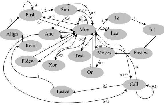
preceded by another instruction MOV, then its count in the matrix with the combination of previous instruction (MOV row) and current instruction (ADD column), will be increased. For example, Table 4 shows a code segment, based on which, a matrix will be created. The total number of distinct instructions is 17 and those are listed below. All distinct instructions will represent an individual node in the graph. All these instructions push, mov, sub, and, test, jz, int, fnstcw, movzx, or, fldcw, call, leave, retn, align, xor, and lea will have outgoing and incoming edges representing some numbers which are counts of those instructions coming after each other.
Instruction (Operator) Operand
Push Ebp
Mov ebp, esp
Sub esp, 8
And esp, 0FFFFFFF0h
Mov eax, ds:dword_404000
Test eax, eax
Jz Short loc_401013
Int 3
Fnstcw [ebp+var_2]
Movzx eax, [ebp+var_2]
And eax, 0FFFFF0C0h
Mov [ebp+var_2], ax
Movzx eax, [ebp+var_2]
Or eax, 33Fh
Mov [ebp+var_2], ax
Fldcw [ebp+var_2]
Mov [esp+8+var_8], offset sub_401050
Call sub_401960
Leave, Retn, Align 10h
Push Ebp
Mov eax, 10h
Mov ebp, esp
Push Edi
Push Esi
Push Ebx
Sub esp, 7Ch
Mov edi, [ebp+arg_0]
Mov esi, [ebp+arg_4]
And esp, 0FFFFFFF0h
Call sub_401930
Call j___main
Mov [ebp+var_4C], 0
Mov [esp+88h+var_88], offset unk_404090
Call j_CORBA_exception_init
Mov dword ptr [esp+88h+var_84+4], esi
Xor edx, edx
Mov eax, offset off_402000
Mov [esp+88h+var_78], edx
Mov [esp+88h+var_7C], eax
Mov dword ptr [esp+88h+var_84], edi
Mov [esp+88h+var_88], offset aOafClient ; "oaf-client"
Call j_poptGetContext
After tracing above instructions and finding all the counts, matrix looks like as shown in Table 5.
Table 5: Matrix created using assembly language instruction counts
In table 5, blank cells represent zeros. Sparse matrix contains more zeros and very less zero values. Thus this matrix becomes a sparse matrix due to less number of non-zero values. Rows in this matrix will represent the nodes and values in that row correspond to values of the edges going out from that node to other nodes. Now if we keep all these counts as it is and calculate the difference, then this technique can easily be defeated. It is because, if we add more and more dead code to the .asm file, it will simply increase the count and will lead to incorrect score.
In a matrix if each row sums to one, then this matrix is called row stochastic matrix. To avoid this problem and to find the probability, we decided to make that matrix, row stochastic. Stochastic matrix is used for non-deterministic or probabilistic calculations
[9]. By taking sum of a row and dividing each value in that row by that sum makes it row stochastic. The sparse row stochastic matrix looks like as shown in table 6.
Table 6: Normalized sparse matrix to make it row stochastic
Table 6 shows the probability of transition from one instruction to another instruction. This way whole successive instruction count is stored in the matrix. Now this matrix can be represented in a graph format as shown in figure 5.
Figure 5: Bi-directed graph created using the matrix in Table 6
Reason behind creating a graph is we want to find the probability of one instruction coming after another or same instruction. After constructing the matrix (graph) for a file, next step is to create another matrix with the counts of successive instructions present in other file. We use the Equation 1 to measure the similarity between two files.
∑ ∑
− = = − = =−
=
1 0 2 1 0 2*
(
(
)
)
1
i N i N j j ij ijb
a
N
Difference
Equation 1: Formula for calculating similarity score [11]
Threshold will be a range or a value which will be useful in classifying benign file and virus file. If the score calculated by this formula is lower than the threshold that means compared files have similar structures in nature. Else if score is higher than the threshold
Push Or Fnstcw Movzx And Jz Test Align Fldcw Leave Int Lea Retn Xor Call Mov Sub 0.4 0.4 0.2 0.05 0.389 0.05 0.05 0.05 0.05 0.167 0.05 0.05 0.5 0.5 0.66 0.33 1 1 1 1 0.5 1 1 0.6 0.2 0.2 1 1 1 1
that means files are different from each other. In this way technique will find whether a given file is a malware or benign software.
4.4 Graph technique algorithm
Below is the algorithm to briefly explain the proposed graph technique. 1.Trace assembly language instructions for the first file
2. Initialize an array with most frequent assembly language instructions present in an “InstSet.txt” file.
2. Create a matrix with memory allocated for all instructions in the above array and initialize all cells with zero.
3. The matrix will be appended dynamically whenever a new instruction is found
4. While tracing the program, keep counting the number of successive instructions which are coming after each other. Store this count in the matrix.
5. Repeat steps 3 and 4 until it reaches end of the file. 6. Repeat steps from 1 through 5 for another file.
7. To calculate the similarity score between these two files (matrices), use the formula in Equation 1.
8. This similarity score will decide whether the given files are similar or different.
4.5 Flow of the graph technique
Figure 6 shows the flow of the graph technique implementation. Combinations of any two files from the following sets will become inputs to the program. A simple text file
module which calculates the similarity score. This score is then used to classify whether the files are similar or different.
Figure 6: Flow of the graph technique
5. Similarity score calculation and analysis
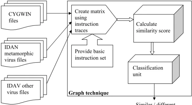
5.1 Data collection
Three different sets are used to test our graph technique. First set has 200 IDAN virus files which belong to one metamorphic virus family. Second set consists of 41 benign files which are nothing but CYGWIN files [13]. Third set contains 25 different virus files. These files do not belong to any family. All these sets were created in [6] to analyze HMM based detection technique.
CYGWIN files IDAN metamorphic virus files IDAV other
virus files Graph technique
Create matrix using instruction traces Provide basic instruction set Calculate similarity score Classification unit Similar / different
As per results in [6], metamorphic viruses can be detected using HMM based detection technique. But according to [7], this technique can be defeated by few morphing techniques like dead code insertion, junk code insertion, and instruction substitution methods. According to [7], 30% subroutine code insertion similar to dead code insertion evades metamorphic virus detection. Percentage of the subroutine code inserted is calculated as per the total number of instructions present in subroutines of a file.
There are two considerations in choosing this dataset. First consideration is we want to compare this technique with HMM based detection technique [6]. For this we will have to use the same dataset, to adequately compare these two techniques. Second
consideration, as discussed in subsection 3.3, is NGVCK metamorphic viruses have already been tested for variation in their structures of all generations [6].
Our aim is to check if our graph technique works for simple metamorphic virus detection, then next step would be to check if it can be defeated by a morphing engine implemented in [7].
5.2 Test cases
Our program compares two files to find their similarity score. This graph technique is implemented to detect metamorphic viruses. Hence there are four important comparisons of different files.
a. Metamorphic virus versus metamorphic virus
5.2.1 Metamorphic virus versus metamorphic virus
In this combination, we are comparing two metamorphic virus files from the same family (IDAN). We have 200 IDAN metamorphic virus files created using NGVCK. After comparing one metamorphic virus file with another metamorphic virus file, we got around 100 scores.
Figure 7: Similarity scores of metamorphic virus files
Figure 7 shows 100 similarity scores between 200 metamorphic viruses. It shows 0.173 as minimum and 0.525 as maximum score for metamorphic virus files (similar files). In this case, similar file score range is from 0.173 to 0.525.
5.2.2 Normal file versus normal file (benign files)
In this combination, we are comparing two benign (normal) files. We have around 41 benign files representing CYGWIN files. After comparing one CYGWIN file with only one CYGWIN file, we get around 20 scores.
Figure 8: Similarity scores for normal files
Maximum similarity score between benign files is 0.468 and minimum similarity score is 0.023. In both the combinations from 5.2.1 and 5.2.2, scores approximately lie in the range from 0.023 to 0.525.
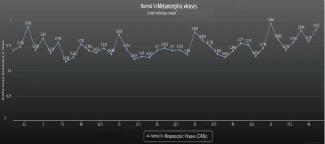
5.2.3 Benign file versus metamorphic virus
This combination is the most important combination. If our graph technique is able to find a similarity score outside the above range, then we will be able to distinguish between metamorphic virus files and benign software files.
For this combination we have 41 instances of benign files and 200 instances of
metamorphic virus files. As this is a one to one comparison, we are using 41 instances of both the files. Figure 9 shows the graph for 41 metamorphic virus files compared with 41
Figure 9: Similarity score for normal versus metamorphic virus file
Figure 10 shows the similarity score between metamorphic virus file and benign file ranges from 0.588 to 0.966. Clearly from above three combinations, metamorphic virus files and benign files are less similar as their scores have higher values as compared to that of two benign files and two metamorphic virus files.
Maximum score range for similar files (two benign files and two metamorphic virus files) is 0.525 and minimum score range for different files (one benign versus one metamorphic virus file) is 0.588. This shows that there is a threshold of 0.063 between similar files and different files. There are one more combinations which are not very important in this scenario, but can be useful in further improvements.
5.2.4 Benign file versus other virus
This combination is also important as the virus we are comparing does not belong to any family. To see if this graph technique is able to detect that this virus and benign files are different, we compared virus file with benign file.
We have 41 benign files and 26 virus files which do not belong to any virus family. To have one to one comparison, we considered 26 virus files and 26 benign files. Figure 10 is the graph created after calculating the scores of 26 virus and benign files.
Figure 10: Graph for normal file versus other viruses
This graph technique also differentiates between normal viruses and normal (benign) softwares. The range of the similarity score is 0.563 to 0.86. This range is closer to the third combination (metamorphic virus Vs benign file) range 0.588 to 0.966. This graph
5.2.5 Combined graph
Figure 11 shows combination of all graphs.
Figure 11: Graph for all types combined
There is a threshold between similar file scores and different file scores. Table 7 shows minimum scores and maximum scores for all cases explained till now.
Metamorphic files versus metamorphic files
Minimum Score Maximum Score
Similar Files 0.173 0.525
Benign files versus benign files
Minimum Score Maximum Score
Similar Files 0.023 0.468
Benign files versus metamorphic files
Minimum Score Maximum Score
Different Files 0.588 0.966
Benign files versus other viruses
Minimum Score Maximum Score
Different Files 0.563 0.860
We have compared files with one to one mapping. But now we will compare one file with all other files using many to many mapping.
5.3 Comparing 10 benign files with 10 metamorphic files
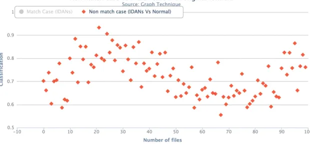
For this combination, we are taking 10 benign files and 10 metamorphic virus files. We will get 100 different observations from many to many comparisons. Figure 12 shows graph of 100 scores for 20 different file combinations. In figure 12, match case is grayed out as those records are temporarily disabled to show only non-match case. Figure 15 shows the complete graph.
Figure 12: Showing graph for normal file versus metamorphic virus file
Minimum score here is 0.555 and maximum score is 0.933. Score 0.555 is greater than 0.525 which is the maximum score for similar files. Graph technique easily identifies
5.3.1 Average score calculation
If we take the average of 10 scores for a particular file compared with different type of files, we can surely differentiate between metamorphic virus files and benign files using this graph technique. We took average of each benign file by adding all ten scores and dividing it by 10. It can be seen in figure 13.
Figure 13: Graph plotted after average score calculations
In figure 13 minimum average score is 0.6464 and maximum average score is 0.844. Minimum average score is larger than threshold 0.525. Before taking average, minimum score was 0.555 which was closer to threshold 0.525 as compared to the minimum average score of 0.6464. It gives confirmed results of similarity or differentiation.
5.4 Comparing 10 metamorphic virus files
Mapping for this comparison will be many to many. Any two metamorphic virus files compared with each other using this graph technique will give the same score even if order of the files is changed. So here we will get 45 distinct scores from many to many mapping of 10 virus files. Figure 14 shows the graph with non-match case disabled (grayed out). Figure 15 shows the complete graph.
Figure 15: Graph showing match and non-match case together
Figure 15 shows both match case versus non-match case. There is a threshold of 0.06 between match case and non-match case. No false positives or false negatives were found.
But now there is a need to check if the formula is effective for metamorphic virus detection. To test its strength, we made some changes in parameters of the formula and calculated the scores with one to one mapping between a set of 41 benign files and metamorphic virus files and another set of 100 metamorphic virus files.
5.5 Parameter variations in the formula
5.5.1 First variation
Now we need to test formula for its strength. In the first variation, we took the square of the difference and then went on adding it to the cumulative sum.
∑ ∑
− = = − = =−
=
1 0 2 1 0 2*
(
(
))
1
i N i N j j ij ijb
a
N
Difference
Equation 2: Squaring the difference and taking the summation
This change in the formula is tested against the same dataset. After calculating score using this changed formula, graph in figure 16 was plotted. Normal file option is disabled for time being.
Figure 16: Result of first variation for match case
The scores for similar files are ranging from 0.003 to 0.007. Scores for different files are shown in figure 17.
Figure 17: Result of first variation for non-match case
Scores are ranging from 0.0054 to 0.0085.
Minimum Score Maximum Score
Similar Files 0.003 0.007
Different Files 0.0054 0.0085
Table 8: First variation scores
Threshold = 0.006
False Positives 2
False Negatives 17
Figure 18: Result of first variation
In figure 18, scores are overlapping for different and similar files. This formula change is not much effective, as there are many false negatives though less false positives.
5.5.2 Second variation
In this variation, we are keeping the above change as it is but removing n2 from it. As n is
the total number of distinct instructions present in both the files, it might not affect much in similarity score.
∑ ∑
− = = − = =−
=
1 0 2 1 0))
(
(
N i i N j j ij ijb
a
Difference
Equation 3: Removed n2 from Equation 2
Figure 19: Result of second variation
Minimum Score Maximum Score
Similar Files 10.241 26.072
Different Files 25.159 48.695
Table 10: Second variation scores
Threshold = 25
False Positives 0
False Negatives 2
Table 11: Second variation - false positives and negatives
Figure 18 and figure 19 show that this formula also works but not as accurate as the formula in equation 1, that is, no threshold to differentiate between similar or different files but very less false positives and negatives.
5.5.3 Third variation
In this change, we are removing n2 from Equation 1. For every score calculation, we are
dividing by the square of the total number of distinct instructions present in both the files. The value of n is approximately similar in all the cases. The score might not get affected due to removal of the n2 term.
∑ ∑
− = = − = =−
=
1 0 2 1 0)
)
(
(
N i i N j j ij ijb
a
Difference
Equation 4: Removing n2 from Equation 1
Figure 20: Result of third variation
The only difference is that values are in thousands range with a separation of 146 and no false positives or false negatives.
5.5.4 Fourth variation
Till now we have seen that value of n2 does not affect much. Another small change could
be removing n2 and only keeping n which is nothing but total number of distinct
instructions present in both the files.
∑ ∑
− = = − = =−
=
1 0 2 1 0)
)
(
(
*
1
i N i N j j ij ijb
a
N
Difference
Equation 5: Keeping only n in Equation 1
Figure 21: Result of fourth variation
Minimum Score Maximum Score
Similar Files 10.087 33.083
Different Files 37.659 77.971
Table 13: Fourth variation score
5.5.5 Fifth variation
In this variation, the term n2 is kept constant as (110)2 and graph is plotted in figure 22.
∑ ∑
− = = − = =−
=
1 0 2 1 0 2*
(
(
)
)
)
110
(
1
i N i N j j ij ijb
a
Difference
Equation 6: Replaced N2 with (110)2 in Equation 1
Figure 22: Result of fifth variation
Though there are no false positives or negatives present, threshold 0.012 is not larger enough. This proves that Equation 1 is more effective.
Minimum Score Maximum Score
Similar Files 0.048 0.172
Different Files 0.184 0.56
6. Observations
From all above test cases, we observed that the graph technique differentiates between metamorphic virus files and benign files.
Graph technique was tested against many types of files. The similarity score distinguishes between similar and non-similar files. When two virus files not belonging to any virus family are compared, results show that their score fall in similarity range. When two metamorphic virus files from the same family are compared, again the score falls in the similarity range. When two benign files are compared against each other, score classifies them as similar files.
But when a benign file is compared against a simple virus or metamorphic virus, results immediately show that it belongs to different score range. When this score calculation is computed using variations in the formula, all figures from section 5.5 show that formula in equation 1 fits the best as compared to other variations.
Figure 23: Equation 1 results for both the cases
Parameter Variations Threshold False Positives False Negatives Score range
Without variation 0.063 0 0 0.173 – 0.966 First variation NA 2 17 0.003 – 0.0085 Second variation NA 0 2 10.241 – 48.695 Third variation 146 0 0 585.056 – 6783.549 Fourth variation 4.576 0 0 10.087 – 77.971 Fifth variation 0.012 0 0 0.048 – 0.56
Table 15: Comparison between parameter variations
To check which variation was the most effective, all score ranges are normalized. Parameter variation 1 and 2 are removed from the comparison as there is no clear threshold between similar and different files. Table 16 shows all threshold values.
Parameter variation Threshold False Positives False Negatives Score range
Without variation 0.0630 0 0 0.173 – 0.966
Third variation / 10000 0.0146 0 0 0.0585 – 0.6783
Fourth variation / 100 0.0457 0 0 0.1008 – 0.7797
Fifth variation 0.0120 0 0 0.048 – 0.56
7. Analysis of graph technique
Following are the key features of this technique.• Common instruction is present in both the files. Range of total difference for a common instruction (row) is 0 to 2.
• The sparse matrix is normalized to make it a row stochastic matrix. This
normalization helps in calculating the probability of similarity. If the matrix is not normalized, then this technique can be attacked by increasing the number of instructions using dead or junk code insertions.
• If an instruction is present in one file but not in the other file, then it is a distinct instruction. The difference of rows representing distinct instructions is one.
Due to all the above features, detection rate of the graph technique is close to 100%. HMM virus detection technique [6] was also successful in detecting NGVCK
metamorphic virus files. But HMM detection technique failed when morphing engine implemented in [7] was used to morph metamorphic virus copies by inserting 30% of dead and junk code.
Next step in this project is to create an attack on this graph technique by compromising its features and by using morphing engine from [7] to morph metamorphic virus files.
8. Attacks on the graph technique
A metamorphic virus file may contain some instructions which are uncommon (not present) in benign files. If we try to replace or remove those instructions to make metamorphic virus file look like a benign file, then test that virus file against a benign file. This might give us score which falls in the similar score range. Removing such instructions will also lower the score.
8.1 Removing distinct instructions
Distinct instructions which are not present in benign file but present in virus file are removed from the virus file to make it look like a normal file. Almost 80% of distinct instructions are removed from a virus file, and scores are calculated. Figure 24 shows the different file scores before and after the attack.
Minimum Score Maximum Score
Score before the attack 0.588 0.966
Score after the attack 0.511 0.94
Table 17: Different file scores
Minimum score fell below the threshold for different files. There is one false negative. Threshold = 0.5
False Positives 0
False Negatives 1
Table 18: Number of false positives / negatives after the attack
From table 18 it is clear that, this attack is able to remove the threshold but it is not successful in defeating the virus detection.
8.2 Using a morphing engine
8.2.1 Morphing engine based on subroutine code insertion and
instruction substitution
In [7], morph engine results are really good in terms of junk and subroutine code insertions. Dead instructions are a set of instructions which are intentionally kept at a place where control never comes and those instructions will not be executed. False loop condition is never true and control does not enter in the loop through out the execution. When dead instructions are placed into the code segment, they do not get executed due to a new jump or a false loop condition. In [7], junk code insertion denotes dead instructions added in between a code segment. Before the dead instructions, a new jump instruction is added which points to the original code and avoids dead code execution. There is one more type of dead code insertion which is subroutine code insertion. A function in the morphing engine copies subroutines from normal file and pastes it into the virus copy to make it look similar to the normal file. As this subroutine is not called anywhere in the virus file, it becomes a dead code. Instruction substitution though not carried out on a higher percentage, morphs the virus copy. Instruction substitution is not of much importance here as it constitutes to 2-3% of the complete code.
Here we have two major cases, junk code insertion and subroutine insertion. After
modifying the morphing engine in [7] to satisfy current requirements, scores for 30% and 40% morphing are calculated and following is a 30% morphed graph.
Figure 26: 30% subroutine code inserted in metamorphic virus files
In figure 26, similar file scores are getting merged with different file scores at some extent. Almost 4 files fall into false positive range. Similarly figure 27 is a graph for 40% subroutine code insertion case. It seems that this attack performs better than instructions removal attack.
8.2.1.1 Comparing HMM and graph based detection
We will compare these results with the results stated in [7]. Figure 28 shows the result for 30% subroutine code insertion tested against HMM based detection technique.
Minimum score Maximum score
Similar Files 0.173 0.525
Different Files 0.428 0.926
Table 19: Scores for graph based technique
False Positive False Negative
4 0
Table 20: False positives / negatives in graph based technique
Table 19 and 20 shows results of our graph technique for morphed metamorphic viruses.
False Positives False Negatives
35 36
Figure 28: HMM based detection results with 30% subroutines copied [7]
Table 21 and Figure 28 show that HMM virus detection technique was failing for 30% subroutine copying from normal file. But our graph technique works much better as compared to HMM based detection technique. Graph based detection technique has 4 false positives. In [7], HMM based detection failed for 30% subroutine code with 36 false negatives and 35 false positives. This way, second attack is also failing to break our graph technique and to evade virus detection.
8.2.2 Morphing engine based on block dead code insertion
In the block morphing, we are capturing a random block from benign file and appending that code into metamorphic virus. The size of the block depends upon the inputs such as percentage of morphing, virus and benign files, and the file sizes. First we need to count the total number of lines present in the virus file. To count the number of lines, we parse
the whole virus file ignoring comments, variable declarations, and blank lines. Then according to the given percentage input we calculate the total number of lines to be copied. Percentage value ranges from 0 to 1. For example, if the percentage value entered is x and total number of actual instruction lines is n, then total number of lines to be copied from benign file is n * x. If n is 700 and x is 0.2 then total number of lines copied from a benign file is 140. After appending the chunk of code in the metamorphic virus file, we calculate the similarity score for the metamorphic virus file as well as the benign file from which the chunk of code is copied. Figure 29 shows scores for all 40 morphed metamorphic viruses scored against 40 benign files for percentages ranging from 0.1 to 1.
Figure 29: Scores for block morphed metamorphic viruses
There is huge drop in scores for different kind of files. For 100% of morphing, the score is below the threshold of 0.525. Till 30%, scores are not affected much. There are only 4 false positives and 6 false negatives as shown in figure 30.
Figure 30: Metamorphic and benign versus morphed metamorphic virus
These scores are calculated when a morphed metamorphic virus is compared with the benign file from which the chunk of code is copied. Hence these two files look similar as we increase the percentage. Figure 31 shows a graph where metamorphic virus file is compared with the benign file from which the code is not copied.
In figure 31, most of the scores are above the threshold of 0.5. It shows that even if the metamorphic virus file is morphed using benign code, it still can be detected using this graph technique.
8.2.2.1 Comparing HMM and graph based detection for block morphing
For this comparison, we have calculated scores individually for all block morphed copies of metamorphic virus files and benign files. To calculate HMM scores we used the HMM detector from [6]. Around 800 scores were calculated for benign files and metamorphic virus files for all percentage cases. Figure 32 shows 30% block morphed scores for metamorphic virus files and benign files.
Figure 32: HMM - 30% block morphed scores
In figure 32, there are many false positives and false negatives.
Minimum score Maximum score
Morphed Metamorphic files -2.620 -43.488
From table 22, it is clear that all benign file scores lie inside the range of morphed metamorphic virus file scores. HMM is not able to distinguish between virus and benign files as there is no clear threshold to distinguish. If we consider a particular threshold of say -3.800 where > -3.800 are metamorphic virus files and < -3.800 are benign files, then values of false positives and false negatives are calculated as shown in table 23.
False Positive False Negative
1 9
Table 23: HMM - 30% false scores
Values of false positives and false negatives depend upon the threshold. If we increase or decrease the particular threshold then false scores are affected. Table 24 shows the false scores for 100% block morphing.
Figure 33: HMM - 100% block morphed results
Here if we consider threshold of -5.000 then table 24 shows the counts of false positives and false negatives.
False Positive False Negative
11 3
Table 24: HMM - 100% false scores
From above figures and tables, it is clear that block morphing is not able to completely evade HMM based metamorphic virus detection. When we compare HMM based detection with graph based detection against block morphing engine, graph based detection is definitely more accurate than HMM as the numbers of false positives and false negatives are very less in case of graph based detection.
8.2.3 Morphing engine based on random dead code insertion
In the random morphing, we are capturing a random block from benign file and evenly distributing the whole chunk of instructions into metamorphic virus. The size of the chunk depends upon the inputs such as percentage of morphing, virus and benign files, and the file sizes. It is similar to block morphing in calculating the total number of lines present in the virus file. Then according to the given percentage input we calculate the total number of lines to be copied. Percentage calculation is also similar to block
morphing. Main difference between these two morphing engines is how the metamorphic virus file morphed using the code copied from benign file. In random morphing, the copied code is evenly distributed through out the metamorphic virus file depending upon a factor “after_lines”. Value of “after_lines” is calculated by dividing length of the virus file with total number of lines to be copied. For example if the morphing percentage is 100% then each statement from the chunk of code is inserted after eac
![Figure 1: Metamorphic virus generations [32]](https://thumb-us.123doks.com/thumbv2/123dok_us/1076947.2643323/18.918.260.675.381.842/figure-metamorphic-virus-generations.webp)