Regression
Yong Zhuang, Wei-Sheng Chin, Yu-Chin Juan, and Chih-Jen Lin Department of Computer Science
National Taiwan University, Taipei, Taiwan
{r01922139,d01944006,r01922136,cjlin}@csie.ntu.edu.tw
Abstract. Regularized logistic regression is a very useful classification method, but for large-scale data, its distributed training has not been investigated much. In this work, we propose a distributed Newton method for training logistic re-gression. Many interesting techniques are discussed for reducing the communi-cation cost and speeding up the computation. Experiments show that the proposed method is competitive with or even faster than state-of-the-art approaches such as Alternating Direction Method of Multipliers (ADMM) and Vowpal Wabbit (VW). We have released an MPI-based implementation for public use.
1
Introduction
In recent years, distributed data classification becomes popular. However, it is known that a distributed training algorithm may involve expensive communication cost be-tween machines. The aim of this work is to construct a scalable distributed training algorithm for large-scale logistic regression.
Logistic regression is a binary classifier that has achieved a great success in many fields. Given a data set withl instances(yi,xi), i = 1, . . . , l, whereyi ∈ {−1,1}is
the label and xi is an n-dimensional feature vector, we consider regularized logistic
regression by solving the following optimization problem to obtain the modelw.
minw 12kwk2+CP
l
i=1logσ(yiwTxi), (1)
whereσ(yiwTxi) = 1 + exp(−yiwTxi)andCis the regularization parameter.
In this paper, we design a distributed Newton method for logistic regression. Many algorithmic and implementation issues are addressed in order to reduce the communi-cation cost and speed up the computation. For example, we investigate different ways to conduct parallel matrix-vector products and discuss data formats for storing feature values. Our resulting implementation is experimentally shown to be competitive with or faster than ADMM and VW, which were considered state-of-the-art for distributed ma-chine learning. Recently, Lin et al. [12] implement a variant of our approach on Spark1 through private communication, but they mainly focus on the efficient use of Spark.
This paper is organized as follows. Section 2 discusses existing approaches for dis-tributed data classification. In Section 3, we present our implementation of a disdis-tributed Newton method. Experiments are in Section 4 while we conclude in Section 5.
2
Existing Methods for Distributed Classification
Many distributed algorithms have been proposed for linear classification. ADMM has recently emerged as a popular method for distributed convex optimization. Although ADMM is a known optimization method for decades, only recently some (e.g., [3, 19]) show that it is particularly suitable for distributed machine learning. Zinkevich et al. [20] proposed a way to parallelize stochastic gradient methods. Besides, parallel coor-dinate descent methods have been considered for linear classification (e.g., [2, 4, 14]). Agarwal et al. [1] recently report that the package VW [9] is scalable and efficient in distributed environments. VW applies a stochastic gradient method in the beginning, then switches to parallel LBFGS [13] for a faster final convergence.
In the rest of this section, we describe ADMM and VW because they are considered state-of-the-art and therefore are involved in our experiments.
2.1 ADMM for Logistic Regression
Zhang et al. [19] apply ADMM on linear support vector machine with squared hinge loss. Here we modify it for logistic regression. Assume data indices{1, . . . , l}are par-titioned to J sets M1, . . . , MJ to indicate data on J machines. We can rewrite the
problem (1) to the following equivalent form.
minw1,...,wJ,z 1 2kzk 2+CPJ j=1 P i∈Mjlogσ(yiwTjxi) subject to z=wj, j= 1, . . . , J. (2)
All optimalz,w1, . . . ,wJ are the same as the solution of the original problem (1).
ADMM repeatedly performs (3)-(5) to update primal variableswandz, and Lagrangian dual variableµusing the following rules.
wk+1j = arg minwj ρ 2kwj−z k−µk jk2+C P i∈Mjlogσ(yiwTjxi), (3) zk+1= arg minz 12kzk2+ρ2P J j=1kz−w k+1 j k 2+ρPJ j=1(µ k j)T(z−w k+1 j ), (4) µk+1j =µk+1j +zk+1−wk+1 j , (5)
whereρ >0is a chosen penalty parameter. Depending on local data, the local model wjon thejth machine can be independently updated using (3). To calculate the
closed-form solution ofzin (4), each machine must collect local modelswj,∀j,so anO(n)
amount of local data from each machine is communicated across the network. The iterative procedure ensures that under some assumptions, ask→ ∞,{zk}approaches
an optimum of (1).
Recall that the communication in (4) involvesO(n)data per machine. Obviously the cost is high for a data set with a huge number of instances (i.e.,nl). Fortunately, Boyd et al. [3] mention that splitting the data set across its features can transform the scale of the communicated data toO(l). For example, if we haveJ machines, the data matrixXis partitioned toX1, . . . , XJ. Note that
X = [x1, . . . ,xl]T = [X1, . . . , XJ].
2.2 VW for Logistic Regression
VW [1] is a machine learning package supporting distributed training. Firstly, by using only local data at each machine, it applies stochastic gradient method with adaptive learning rate [5]. Then, to get a faster convergence, VW weightedly averages the model as the initial solution for the subsequent quasi Newton method [13] on the whole data. The stage of applying stochastic gradient updates goes through all local data once for approximately solving the following sub-problem.
P i∈Mj( 1 2kwk 2+Clogσ(y iwTxi)).
In the second stage, the objective function of (1) is considered and the quasi Newton method applied is LBFGS, which usesmvectors to approximate inverse Hessian (mis a user-specific parameter). To support both numerical and string feature indices in the input data, VW uses feature hashing to have a fast feature lookup. That is, it applies a hash function on the feature index to generate a new index for that feature value.
We discuss the communication cost of VW, which supports only the instance-wise data split. For the stage of running a stochastic gradient method, there is no communi-cation until VW weightedly averages localwj,∀j, whereO(n)data on each machine
must be aggregated. For LBFGS, it collectsO(n)results on each machine to calcu-late the function value and the gradient. Therefore, the communication cost per LBFGS iteration is similar to that of each ADMM iteration under the instance-wise data split.
3
Distributed Newton Methods
In this section, we describe our proposed implementation of a distributed Newton method.
3.1 Newton Methods
We denote the objective function of (1) asf(w). At each iteration, a Newton method updates the current modelwby
w←w+s, (6)
wheres, the Newton direction, is obtained by minimizing
mins q(w), q(w) =∇f(w)Ts+12sT∇2f(w)s. (7)
Because the Hessian matrix∇2f(w)is positive definite, we can solve the following
linear system instead.
∇2f(w)s=−∇f(w). (8) For data with a huge number of features, ∇2f(w)becomes too large to be stored.
Hessian-free methods have been developed to solve (8) without explicitly forming ∇2f(w). For example, Keerthi and DeCoste [8] and Lin et al. [11] apply conjugate
gradient (CG) methods to solve (8). CG is an iterative procedure that requires a Hessian-vector product∇2f(w)vat each step. For logistic regression, we note that
∇2f(w)v=v+CXT(D(Xv)), (9)
whereDis a diagonal matrix with Dii =
σ(yiwTxi)−1
σ(yiwTxi)2
Xiw,1 Xiw,2 Xiw,3
(a) Instance-wise (IW)
Xfw,1Xfw,2Xfw,3
(b) Feature-wise (FW) Fig. 1: Two methods to distributedly store training data.
From (9), we can clearly see that a sequence of matrix-vector products is sufficient to finish the Hessian-vector product. Because ∇2f(w)is not explicitly formed, the
memory difficulty is alleviated.
The update (6) does not guarantee the convergence to an optimum, so we apply a trust region method [11]. A constraintksk2≤∆is added to (7), where∆is called the
radius of the trust region. At each iteration, we check the ratioρin (10) to ensure the reduction of the function value.
ρ=f(w+s)−f(s)
q(w) . (10)
Ifρis not large enough, thensis rejected andwis kept. Otherwise,wis updated by (6). Then, the radius∆is adjusted based onρ[11].
Although Hessian-vector products are the main computational bottleneck of the above Hessian-free approach, we note that in Newton methods other operations such as function and gradient evaluations are also important. For example, the function value in (1) requires the calculation ofXw. Based on this discussion, we can conclude that a scalable distributed Newton method relies on the effective parallelization of multiplying the data matrix with a vector. We will discuss more details in the rest of this section.
3.2 Instance-wise and Feature-wise Data Splits
Following the discussion in Section 2.1, we may split training data instance-wisely or feature-wisely to different machines. An illustration is in Figure 1, in whichXiw,j or
Xfw,j represents thejth segment of data stored in thejth machine. We will show that
the two splits lead to different communication cost. Subsequently, we use “IW/iw” and “FW/fw” to denote instance-wise and feature-wise splits.
To discuss the distributed operations easily, we use vector notation to rewrite (1) as f(w) =1
2kwk
2+Clog(σ(Y Xw))
·e, (11)
whereXandY are defined in Section 2.1,log(·)andσ(·)are component-wisely applied to a vector, and “·” stands for a dot product. In (11),e∈Rn×1is a vector of all ones.
Then the gradient can be represented as
∇f(w) =w+C(Y X)T(σ(Y Xw)−1−e). (12) Next we discuss details of distributed operations under the two different data splits.
Instance-wise Split: Based on (9)-(12), the distributed form of function, gradient val-ues, and Hessian-vector products can be written as
f(w) =12kwk2+CLJ
∇f(w) =w+CLJ j=1(YjXiw,j)T(σ(YjXiw,jw)−1−ej), (14) and ∇2f(w)v=v+CLJ j=1X T iw,jDjXiw,jv, (15)
whereYj,ej, andDjare respectively the sub-matrix, the sub-vector, the sub-matrix of
Y,e, andDcorresponding to instances in thejth machine. We useL
to denote an all-reduceoperation [15] that collects results from all machines and redistributes the sum to them. For example,LJ
j=1log(σ(YjXiw,jw))means that each machine calculates its
ownlog(σ(YjXiw,jw)), and then anall-reducesummation is performed. Feature-wise Split: We notice that
Xw=LJ
j=1Xfw,jwj, (16)
wherewj is a sub-vector of w corresponding to features stored in the jth machine.
Therefore, in contrast to IW, each machine maintains only a sub-vector ofw. The situ-ation is similar to other vectors such ass. However, to calculate the function value for checking the sufficient decrease (10),kwjk2,∀jmust be summed and then distributed
to all machines. Therefore, the function value is calculated by
1 2 LJ j=1kwjk 2+Clog(σ(Y LJ j=1Xfw,jwj))·e. (17)
Similarly, each machine must calculate part of the gradient and the Hessian-vector prod-uct: ∇f(w)fw,p=wp+C(Y Xfw,p)T(σ(Y L J j=1Xfw,jwj) −1 −e) (18) and (∇2f(w)v) fw,p=vp+CXfw,TpD LJ j=1Xfw,jvj,
where, likew, only a sub-vectorvpofvis needed at thepth machine.
We notice that someall-reduceoperations are needed for inner products in Newton methods. For example, to evaluate the value in (7) we must obtain
∇f(w)Ts=LJ
j=1∇f(w) T
fw,jsj, (19)
where∇f(w)fw,j andsj are respectively the sub-vectors of∇f(w)andsstored at
thejth machine. The communication cost is not a concern because (19) sumsJvalues rather than vectors in (16). Another difference from the IW approach is that the label vectoryis stored in every machine because of the diagonal matrixY in (17) and (18). It is worth mentioning that to save computational and communication cost, we can cache LJ
j=1Xfw,jwjobtained in (17) for (18).
Analysis: To compare the communication cost between IW and FW, in Table 1 we show the number of operations at each machine and the amount of data sent to all others. From Table 1, to minimize the communication cost, IW and FW should be used forlnandnl, respectively. We will confirm this property through experiments in Section 4.
#of operations #data sent to other machines IW FW IW FW f(w) O(nnz/J)O(nnz/J) O(1) O(l) ∇f(w) O(nnz/J)O(nnz/J)O(n) 0 ∇2 f(w)v O(nnz/J)O(nnz/J)O(n) O(l) inner product O(n) O(n/J) 0 O(1)
Table 1: A comparison between IW and FW on the amount of data distributed from one machine to all others.J is the number of machines and nnz is the number of non-zero elements in the data matrix. For FW, the calculation of∇f(w)does not involve com-munication because we mentioned thatLJ
j=1Xfw,jwj is available while calculating
f(w).
3.3 Other Implementation Techniques
Load Balancing: The parallel matrix-vector product requires that all machines finish their local tasks first. To reduce the synchronization cost, we should let machines have a similar computational load. Now the computational cost is related to the number of non-zero elements, so we split data in a way such that each machine contains data of a similar number of non-zero values.
Data Format: Lin et al. [11] discuss two approaches to store the sparse data matrix X in an implementation of Newton methods: compressed sparse row (CSR) and com-pressed sparse column (CSC). They conclude that because of the possibility of storing a whole row or column into a higher-level memory (e.g., cache), CSR and CSC are more suitable forl nandn l, respectively. Because we split data so that each machine has a similar number of non-zero elements, the number of columns/rows of the sub-matrix may vary. In our implementation, we dynamically decide the sparse format based on if the sub-matrix’s number of rows is greater than columns.
Speeding Up Hessian-vector Product: Instead of sequentially calculatingXv,D(Xv), andXT(D(Xv))in (9), we can re-writeXTDXvas
Pl
i=1Dii(xi(xTiv)). (20)
Then the data matrixXis accessed only once rather than twice. However, this technique can only be applied for instance-wisely split data in the CSR format. If the data is split by features, then calculating eachxTivneeds anall-reduceoperation. Thelall-reduce
summations in (20) cause too high communication cost in practice.
4
Experiments
In this section, we begin with describing a specific Newton method used for our imple-mentation. Then we evaluate techniques proposed in Section 3, followed by a detailed comparison between ADMM, VW, and the distributed Newton method on objective function values and test accuracy.
4.1 Truncated Newton Method
In Section 3.1, using CG to find the directionsmay struggle with too many iterations. To alleviate this problem, we consider an approach by Steihaug [16] that employs CG to approximately minimize (7) under the constraint ofsbeing in the trust region. With the Newton directionsobtained approximately, the technique is called a truncated Newton
Data set l n #nonzeros C Communication Total IW FW IW FW yahoo-japan 140,963 832,026 18,738,315 0.5 166.22 13.78 169.73 15.15 yahoo-korea 368,444 3,052,939 125,190,807 2 1,185.32 189.72 1,215.76 207.53 url 2,396,130 3,231,961 277,058,644 2 9,727.896,995.2310,194.237,286.63 epsilon 500,000 2,000 1,000,000,000 2 2.16 184.03 11.37 195.26 webspam 350,000 16,609,143 1,304,697,446 32 8,909.51 159.83 9,179.42 199.36
Table 2:Left:The statistics of each data set.Right:Communication and total running time (in seconds) of the distributed Newton method using IW and FW strategies. method. Lin et al. [11] have applied this method for logistic regression on a single machine. Here we follow their detailed settings for our distributed implementation.
4.2 Experimental Settings
1. Data Sets:We use five data sets listed in Table 2 for experiments, and randomly split them into 80%/20% as training set and test set respectively (an exception is
epsilonbecause it has official training/test sets). Exceptyahoo-japanand
yahoo-korea, all others are publicly available.2
2. Platform:We use 32 machines in a local cluster. Each machine has an 8-core pro-cessor with computing power equivalent to 8 ×1.0GHz 2007 Xeon, and 16GB memory. The network bandwidth is approximately 1Gb/s.
3. Parameters:ForCin (1), we tried different values in{2−5,2−3, . . . ,25}, and use
the one that leads to the best performance on the test set.
4.3 IW versus FW
This subsection presents a comparison between two different data splits. We run the Newton method until the following stopping condition is satisfied:
k∇f(w)k ≤min(pos,neg)
l k∇f(0)k, (21) where= 10−6and pos/neg are the number of positive and negative data.
In Table 2, we present both communication and total training time. Results are con-sistent with our analysis in Table 1. For example, IW is better than FW forepsilon, which has l n. On the contrary, FW is superior for webspambecause l n. This experiment reflects that a suitable data split strategy can significantly reduce the communication cost.
By the difference between total and communication time in Table 2, we have the time for computation and synchronization. It is only similar but not the same for IW and FW because of the variance of the cluster’s run-time behavior and the algorithmic differences.
4.4 Comparison Between State-of-the-art Methods on Function Values
We include the following methods for the comparison.
• the distributed trust-region Newton method (TRON): It is implemented in C++ with OpenMPI [7].
2
• ADMM: We implement ADMM using C++ with OpenMPI [7]. Following Zhang et al. [19], the sub-problem (3) is approximately solved by a coordinate descent method [17] with a fixed number of iterations, where the number of iterations is decided by a validation procedure. The parameterρin (3) follows the setting in [19]. • VW (version 7.6): The package uses sockets for communications and synchroniza-tion. Because VW uses the hashing trick for the features indices, hash collisions may cause not only different training/test sets but also worse accuracy. To reduce the pos-sibility of hash collisions, we set the size of the hashing table larger than the original data sets.3Although the data set may be slightly different from the original one, we
will see that the conclusion of our experiments is not affected. Besides, we observe that the default setting of running a stochastic gradient method and then LBFGS is very slow onwebspam, so for this problem, we apply only LBFGS.4ExceptCand
the size of features hashing, we use the default parameters in VW.
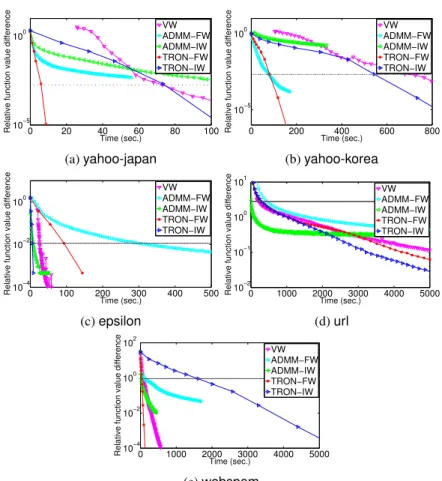
In Figure 2, we compare VW, ADMM, and the distributed Newton method by checking the relation between the training time and the relative distance from the cur-rent function value to the optimum:
|f(w)−f(w∗)| |f(w∗)| .
The reference optimalw∗is obtained approximately by running the Newton method with a very small stopping tolerance.5 We present results of ADMM and distributed
Newton using both instance-wise and feature-wise splits. For the sparse format in Sec-tion 3.3, the distributed Newton method dynamically chooses CSC or CSR, while ADMM uses CSC because of the requirement of the coordinate descent method for the sub-problem (3).
Results in Figure 2 indicate that with suitable data splits, the distributed Newton method converges faster than ADMM and VW. Regarding IW versus FW, whenl n, an instance-wise split is more suitable for the distributed Newton method, while a feature-wise split is better forn l. This observation is consistent with Table 2. However, the same result does not hold for ADMM. One possible explanation is that regardless of data splits, the optimization processes of the distributed Newton method are exactly the same. In contrast, ADMM’s optimization processes are different under IW and FW strategies [3].
In Figure 2, a horizontal line indicates that the stopping condition of (21) with= 0.01has been satisfied. This condition, used as the default condition in the Newton-method implementation of the software LIBLINEAR[6], shows that a model having similar prediction capability to the optimal solution has been obtained. In Figure 2,
3
We select220,222,222,212, and225as the size of the hashing table foryahoo-japan, yahoo-korea,url,epsilon, andwebspamrespectively.
4We observe that the vectorwobtained after running stochastic gradient methods is a poor
initial point for LBFGS to have slow convergence. It is not entirely clear what happened, so further investigation is needed.
5
The optimal solution of VW with hashing tricks may be different from the other two methods, so we obtain itsw∗separately. Because of using the relative distance, we can still compare the convergence speed of different methods.
0 20 40 60 80 100 10−5
100
Time (sec.)
Relative function value difference
VW ADMM−FW ADMM−IW TRON−FW TRON−IW (a)yahoo-japan 0 200 400 600 800 10−5 100 Time (sec.)
Relative function value difference
VW ADMM−FW ADMM−IW TRON−FW TRON−IW (b)yahoo-korea 0 100 200 300 400 500 10−4 10−2 100 Time (sec.)
Relative function value difference
VW ADMM−FW ADMM−IW TRON−FW TRON−IW (c)epsilon 0 1000 2000 3000 4000 5000 10−2 10−1 100 101 Time (sec.)
Relative function value difference
VW ADMM−FW ADMM−IW TRON−FW TRON−IW (d)url 0 1000 2000 3000 4000 5000 10−4 10−2 100 102 Time (sec.)
Relative function value difference
VW ADMM−FW ADMM−IW TRON−FW TRON−IW (e)webspam
Fig. 2: A comparison on the relative difference to the optimal objective function value. The dotted line indicates the stopping conditions (21) with= 0.01has been achieved. ADMM can quickly reach the horizontal line for some problems, but is slow for others.
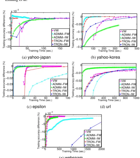
4.5 Comparison Between State-of-the-art Methods on Test Accuracy
We present in Figure 3 the relation between the training time and accuracy−best accuracy
best accuracy ,
where best accuracy is the best final accuracy obtained by all methods. In the early stage ADMM is better than the other two, while the distributed Newton method gets the final stable performance more quickly on all problems excepturl.
4.6 Speedup
Following Agarwal et al. [1], we compare the speedup of ADMM, VW, and the dis-tributed Newton method for obtaining a fix test accuracy by varying the number of machines. Results are in Figure 4.
We consider the two largest setsepsilonandwebspamfor experiments. They have lnandnl, respectively. For ADMM and the distributed Newton method, we use
0 50 100 150 −20 −15 −10 −5 0 x 10−3
Training Time (sec.)
Testing accuracy difference (%)
VW ADMM−FW ADMM−IW TRON−FW TRON−IW (a)yahoo-japan 0 100 200 300 400 500 −0.2 −0.15 −0.1 −0.05 0
Training Time (sec.)
Testing accuracy difference (%)
VW ADMM−FW ADMM−IW TRON−FW TRON−IW (b)yahoo-korea 0 20 40 60 80 100 −0.05 −0.04 −0.03 −0.02 −0.01 0
Training Time (sec.)
Testing accuracy difference (%)
VW ADMM−FW ADMM−IW TRON−FW TRON−IW (c)epsilon 0 200 400 600 800 1000 −0.04 −0.03 −0.02 −0.01 0
Training Time (sec.)
Testing accuracy difference (%)
VW ADMM−FW ADMM−IW TRON−FW TRON−IW (d)url 0 500 1000 1500 2000 −20 −15 −10 −5 0x 10 −3
Training Time (sec.)
Testing accuracy difference (%)
VW ADMM−FW ADMM−IW TRON−FW TRON−IW (e)webspam
Fig. 3: A test-accuracy comparison among ADMM, VW and the distributed Newton method with different data split strategies. The dotted horizontal line indicates 0 differ-ence to the final accuracy.
the data split strategy leading to the better convergence in Figure 2. Figure 4 shows that
for epsilon(l n), VW and the distributed Newton method yield a better speedup
than ADMM as the number of machines increases, while forwebspam(n l), the distributed Newton method is better than the other two.
For the problemwebspam, the speedup of VW is much worse thanepsilonand problems in [1], so we conduct some investigation. Forepsilon and data in [1], they haveln. Thus we suspect that becausenlforwebspamand VW considers an instance-wise split, VW suffers from high communication cost. To confirm this point, we conduct an additional experiment in Figure 4(b). A special property of the problem
webspamis that it actually has only 680,715 non-zero feature columns, although its
feature indices are up to 16 million. We generate a new set by removing zero columns and rerun VW.6 The result, indicated as VW* in Figure 4(b), clearly shows that the
speedup is significantly improved.
6
1 2 4 8 16 32 0 5 10 15 20 Number of machines Speedup VW ADMM−IW TRON−IW (a)epsilon 4 8 16 32 0 1 2 3 4 Number of machines Speedup VW VW* ADMM−IW TRON−FW (b)webspam Fig. 4: The speedup of different training methods.
0 5 10 15 20 −6 −4 −2 0 Iterations
Relative function value difference
Nodes−1 Nodes−2 Nodes−4 Nodes−8 Nodes−16 Nodes−32 (a)epsilon 0 20 40 60 −6 −4 −2 0 2 4 Iterations
Relative function value difference
Nodes−4 Nodes−8 Nodes−16 Nodes−32
(b)webspam
Fig. 5: The relation between the number of ADMM iterations and the decrease of the function value. We show results of using different numbers of machines.
Next, we investigate more about the unsatisfactory speedup of ADMM. Because of parallelizing only the matrix-vector products, the numbers of iterations in VW and the distributed Newton method are independent of the number of machines. In contrast, ADMM’s number of iterations may significantly vary, because the reformulation in (2) is related to the number of machines. In Figure 5, we present the relation between the number of ADMM iterations and the relative difference to the optimum. It can be seen that as the number of machines increases, the higher number of iterations comes with more computational and communication costs. Thus the speedup of ADMM in Figure 4 is not satisfactory.
5
Conclusion
To the best of our knowledge, this work is the first comprehensive study on the dis-tributed Newton method for regularized logistic regression. We carefully address im-portant issues for distributed computation including communication and memory local-ity. An advantage of the proposed distributed Newton method and VW over ADMM is that the optimization processes are independent of the distributed configuration. That is, the number of iterations remains the same regardless of the number of machines. Our experiment shows that in a practical distributed environment, the distributed Newton method is faster and more scalable than ADMM and VW that are considered state-of-the-art for real-world problems.
However, because of requiring differentiability, Newton methods are more restric-tive than ADMM. For example, if we consider L1-regularization by replacingkwk2/2
in (1) with kwk1, the optimization problem becomes non-differentiable, so Newton
methods cannot be directly applied.7
Our experimental code is available at (removed for the blind review requirements).
Bibliography
1. Agarwal, A., Chapelle, O., Dudik, M., and Langford, J. (2014). A reliable effective terascale linear learning system.JMLR, 15:1111–1133.
2. Bian, Y., Li, X., Cao, M., and Liu, Y. (2013). Bundle CDN: a highly parallelized approach for large-scale l1-regularized logistic regression. InECML/PKDD.
3. Boyd, S., Parikh, N., Chu, E., Peleato, B., and Eckstein, J. (2011). Distributed optimization and statistical learning via the alternating direction method of multipliers.Found. Trends Mach. Learn., 3(1):1–122.
4. Bradley, J. K., Kyrola, A., Bickson, D., and Guestrin, C. (2011). Parallel coordinate descent for l1-regularized loss minimization. InICML.
5. Duchi, J., Hazan, E., and Singer, Y. (2011). Adaptive subgradient methods for online learning and stochastic optimization.JMLR, 12:2121–2159.
6. Fan, R.-E., Chang, K.-W., Hsieh, C.-J., Wang, X.-R., and Lin, C.-J. (2008). LIBLINEAR: a library for large linear classification.JMLR, 9:1871–1874.
7. Gabriel, E., Fagg, G. E., Bosilca, G., Angskun, T., Dongarra, J. J., Squyres, J. M., Sahay, V., Kambadur, P., Barrett, B., Lumsdaine, A., Castain, R. H., Daniel, D. J., Graham, R. L., and Woodall, T. S. (2004). Open MPI: Goals, concept, and design of a next generation MPI implementation. InEuropean PVM/MPI Users’ Group Meeting, pages 97–104.
8. Keerthi, S. S. and DeCoste, D. (2005). A modified finite Newton method for fast solution of large scale linear SVMs.JMLR, 6:341–361.
9. Langford, J., Li, L., and Strehl, A. (2007). Vowpal Wabbit. https://github.com/ JohnLangford/vowpal_wabbit/wiki.
10. Lin, C.-J. and Mor´e, J. J. (1999). Newton’s method for large-scale bound constrained prob-lems.SIAM J. Optim., 9:1100–1127.
11. Lin, C.-J., Weng, R. C., and Keerthi, S. S. (2008). Trust region Newton method for large-scale logistic regression.JMLR, 9:627–650.
12. Lin, C.-Y., Tsai, C.-H., Lee, C.-P., and Lin, C.-J. (2014). Large-scale logistic regression and linear support vector machines using Spark. InIEEE BigData.
13. Liu, D. C. and Nocedal, J. (1989). On the limited memory BFGS method for large scale optimization.Math. Program., 45(1):503–528.
14. Richt´arik, P. and Tak´aˇc, M. (2012). Parallel coordinate descent methods for big data opti-mization.Math. Program.Under revision.
15. Snir, M. and Otto, S. (1998). MPI-the complete reference: the MPI core. MIT Press, Cam-bridge, MA, USA.
16. Steihaug, T. (1983). The conjugate gradient method and trust regions in large scale optimiza-tion.SIAM J. Numer. Anal., 20:626–637.
17. Yu, H.-F., Huang, F.-L., and Lin, C.-J. (2011). Dual coordinate descent methods for logistic regression and maximum entropy models.MLJ, 85:41–75.
18. Yuan, G.-X., Chang, K.-W., Hsieh, C.-J., and Lin, C.-J. (2010). A comparison of optimization methods and software for large-scale l1-regularized linear classification.JMLR, 11:3183–3234. 19. Zhang, C., Lee, H., and Shin, K. G. (2012). Efficient distributed linear classification
algo-rithms via the alternating direction method of multipliers. InAISTATS.
20. Zinkevich, M., Weimer, M., Smola, A., and Li, L. (2010). Parallelized stochastic gradient descent. InNIPS.
7An extension for L1-regularized problems is still possible (e.g., [10, 18]), though the algorithm