Continuous Authentication using Inertial-Sensors of Smartphones and Deep Learning

(1)

University of Media Stuttgart

Faculty of Information & Communication Data Science & Business Analytics

Robert Bosch GmbH

Corporate Research Department CR/AEU2

THESIS

Continuous Authentication using

Inertial-Sensors of Smartphones and

Deep Learning

Holger Büch

Mat.-No. 33953

Submitted in partial fulfillment of the requirements for the degree of Master of Science in Data Science & Business Analytics

at the University of Media Stuttgart in June 28th, 2019.

1. Reviewer Prof. Dr. Johannes Maucher

Faculty of Print and Media University of Media, Stuttgart

2. Reviewer Dr. Michael Dambier

Corporate Research, CR/AEU2 Robert Bosch GmbH

Additional Advisor Dr. Robert Duerichen

Corporate Research, CR/AEU2 Robert Bosch GmbH

(2)

Holger Büch

Continuous Authentication using Inertial-Sensors of Smartphones and Deep Learning

THESIS, June 28th, 2019

Reviewers: Prof. Dr. Johannes Maucher and Dr. Michael Dambier Additional Advisor: Dr. Robert Duerichen

University of Media Stuttgart

Data Science & Business Analytics Faculty of Information & Communication Nobelstraße 10

(3)

Declaration

Hiermit versichere ich, Holger Büch, ehrenwörtlich, dass ich die vorliegende Master-arbeit mit dem Titel: “Continuous Authentication using Inertial-Sensors of Smart-phones and Deep Learning” selbstständig und ohne fremde Hilfe verfasst und keine anderen als die angegebenen Hilfsmittel benutzt habe.

Die Stellen der Arbeit, die dem Wortlaut oder dem Sinn nach anderen Werken entnommen wurden, sind in jedem Fall unter Angabe der Quelle kenntlich gemacht. Die Arbeit ist noch nicht veröffentlicht oder in anderer Form als Prüfungsleistung vorgelegt worden.

Ich habe die Bedeutung der ehrenwörtlichen Versicherung und die prüfungsrechtlichen Folgen (§ 17 Abs. 5 der Studien- und Prüfungsordnung berufsbegleitender weit-erführender Studiengänge, 5-semestrig) einer unrichtigen oder unvollständigen ehrenwörtlichen Versicherung zur Kenntnis genommen.

Stuttgart, June 28th, 2019

(4)

(5)

Abstract

The legitimacy of users is of great importance for the security of information systems. The authentication process is a trade-off between system security and user experi-ence. E.g., forced password complexity or multi-factor authentication can increase protection, but the application becomes more cumbersome for the users. Therefore, it makes sense to investigate whether the identity of a user can be verified reliably enough, without his active participation, to replace or supplement existing login processes.

This master thesis examines if the inertial sensors of a smartphone can be leveraged to continuously determine whether the device is currently in possession of its legitimate owner or by another person. To this end, an approach proposed in related studies will be implemented and examined in detail. This approach is based on the use of a so-called Siamese artificial neural network to transform the measured values of the sensors into a new vector that can be classified more reliably.

It is demonstrated that the reported results of the proposed approach can be repro-duced under certain conditions. However, if the same model is used under conditions that are closer to a real-world application, its reliability decreases significantly. There-fore, a variant of the proposed approach is derived whose results are superior to the original model under real conditions.

The thesis concludes with concrete recommendations for further development of the model and provides methodological suggestions for improving the quality of research in the topic of “Continuous Authentication”.

Keywords:Deep Learning, Machine Learning, Sensors, Authentification

(6)

Abstract (German)

Für die Sicherheit von Informationssystemen ist die Legitimierung der Nutzer von großer Bedeutung. Der Authentifizierungsprozess ist dabei eine Gratwanderung zwischen Sicherheit des Systems und Benutzerfreundlichkeit. So können etwa erzwungene Passwortkomplexität oder Multi-Faktor-Authentifizierung den Schutz erhöhen, für Anwender wird die Bedienung jedoch umständlicher. Daher stellt sich die Frage, ob die Identität des Nutzers auch ohne seine aktive Mitwirkung zuverlässig genug verifiziert werden kann, um dadurch Anmeldeprozesse sinnvoll ersetzen oder ergänzen zu können.

In dieser Masterarbeit wird die Frage untersucht, ob mithilfe der Inertialsensoren eines Smartphones kontinuierlich ermittelt werden kann, ob sich das Gerät gerade in Besitz seines rechtmäßigen Eigentümers befindet, oder von einem Dritten getragen wird. Hierzu wird ein in der Forschungsliteratur vorgeschlagener Ansatz nach implementiert und genauer untersucht. Der Ansatz basiert auf der Verwendung eines sogenannten siamesischen künstlichen neuronalen Netzwerks, um die Messwerte der Sensoren in einen anderen Vektor zu transformieren, der zuverlässiger klassifiziert werden kann.

Im Ergebnis wird gezeigt, dass sich die berichteten Ergebnisse des vorgeschlagenen Ansatzes unter bestimmten Voraussetzungen reproduzieren lassen. Wird das gleiche Modell unter Bedingungen eingesetzt, die einer realen Anwendung näher kommen, nimmt die Zuverlässigkeit jedoch massiv ab. Daher wird eine Variante des genutzten Ansatzes hergeleitet, deren Ergebnisse dem ursprünglichen Modell unter realen Bedingungen überlegen sind.

Die Arbeit schließt mit konkreten Empfehlungen zur Weiterentwicklung des Modells und gibt methodische Anregungen zur Qualitätssteigerung der Forschung in diesem Themenfeld der “Continuous Authentication”.

(7)

Introduction

Verifying a user’s identity is crucial for the security of information systems. But the authentication process, in which a person verifies himself as a known and legitimate user of a system, seems to bear an inherent trade-off between reliability and convenience: The convenience of the user decreases if the reliability is improved, e.g., by enforcing complex password rules, multi-factor authentication, or frequent re-authentication. And this is not just a question of comfort, the security of the whole system can suffer from low user acceptance, whether through a written password attached to a computer monitor, a personal physical access token shared between colleagues, deliberately deactivating security features or other workarounds.

Is it possible to validate a user, without the need for his active participation in the authentication process? How can a system continuously collect information provided passively by the user and use unique patterns embedded in this information to identify the user? Does such a system improve the convenience of authentication? How reliable is it, and how does it affect security? Those are common research questions in the field of Continuous Authentication (CA), the topic of this master thesis. Given the omnipresence of personal smartphones, with their steadily increas-ing computational power and a variety of built-in sensors, it seems appropriate for this thesis to focus on leveraging the capabilities of those devices.

The purpose of this thesis is to assess the feasibility of a CA approach which is based on data provided by the inertial sensors of smartphones. Those sensors, gyroscope, accelerometer, and magnetometer, have the advantage to not depend on the active usage of the smartphone, they only need to be able to capture movements produced by the user. This aspect concludes the motivation behind the thesis: If it is possible to authenticate a user through the smartphone without the need for active usage of the device, it will open up the possibility to not only authenticate the user against, e.g., the phones operating system. The authentication state could also be shared with third-party systems, which cannot recognize the user on their own, to benefit from CA through the smartphone.

The research in this thesis focuses on experiments performed on a desktop computer with datasets collected by smartphones up front, and on verifying the ability of different machine learning models to classify the user as legitimate “owner” or

(12)

illegitimate “impostor”. Before this ability is evaluated, further topics seem to be secondary. Therefore, other important tasks like testing the authentication on actual mobile devices, assessing the system’s security against planned attacks, designing an architecture for integration with third-party systems, or keeping the machine learning model up to date have been held out of scope for this thesis.

The idea of using inertial sensors of smartphones for CA already was the topic of many previous studies by different researchers. Such related work is summarized in Chapter 3. While I examined those studies, it became apparent, that most researchers spend a lot of effort into feature engineering, trying to find different representations of the sensor data which can be leveraged effectively as input for machine learning models to classify the sensors’ signals. But with the advancements in the field of Artificial Neural Networks (ANNs), it is tempting to supersede the manual feature engineering with feature learning through deep learning methods.

The promising results published by Centeno et al. (2018) were one of the reasons I decided to reimplement their approach, a combination of a Siamese Convolutional Neural Network (CNN) with an One Class Support Vector Machine (OCSVM), as a significant aspect of this thesis. I elaborate on this and other design decisions, along with further building blocks of my concept, in Chapter 4.

The details of the experiments and the used dataset are presented in Chapter 5. Those experiments include the implementation of an OCSVM baseline model and the mentioned ensemble of a Siamese CNN with an OCSVM, along with an extensive evaluation. Within the experiments, I demonstrate, that the promising reported results are to my best knowledge caused by a setup, which is not applicable in a real-world scenario. I also show that the same models perform significantly weaker if the conditions of a real-world scenario are applied. Further, I evaluate the impact of various model parameters and propose a variation of the original model with improved performance in conditions closer to real-world scenarios, but without getting near the performance reported in the original study.

In Chapter 6, I discuss significant findings I discovered while working on this thesis, propose questions for future research, and make suggestions on how the research in CA could be improved in general.

But before deep diving into the topic of this thesis, the next Chapter 2 introduces into basic aspects specific to the examined subject.

(13)

2

Basics

The first section in this chapter explains and contextualizes the domain of this thesis: behavioral biometrics based Continuous Authentication. The second section describes the functional principles and constraints of the smartphone sensors relevant for this thesis to improve the understanding of the data they produce.

2.1

Access Control and Authentication

To protect a computing system against illegitimate access, it has to be equipped with some kind of control mechanism. To pass this mechanism, the user has to follow a specific process containing multiple steps or sub-processes. This topic is too complex to be cover in detail in this thesis. The following subsections focus on the aspects needed to understand and judge the approach of CA as the topic of this thesis. The three aspects most relevant for this thesis are: The general process of access control including authentication, the source of information which is used to perform authentication, and the frequency of authentication with its impact on security and convenience. For a more detailed examination of authentication, refer to Dasgupta et al. (2017).

2.1.1

Access Control Process

The process of gaining access to a computing system usually consists of multiple steps or subprocesses. These often include at least the following three subsequent steps: identification, authentication, and authorization.

Identification is the process where the user has to proof his “true” identity, e.g., his legal identity as a citizen by showing his official passport, or his identity as the owner of a specific e-mail account by entering a piece of secret information that has been sent to that account (Dasgupta et al., 2017, p. 2). Often identification is only needed during an initial registration process or if irregularities question the true identity. Authentication is the process in which the user provides information to verify that he, as a user, is a person with an already proven “true” identity. Usually, this information

(14)

contains an identifier and a secret like a username and a password. Dasgupta et al. (2017, p. 2) define this process as follows:

“Authentication is the mandatory process to verify the identity of a user and restricts illegitimate users to access the system.”

Authorization is the process of granting or denying access right to the authenticated user, respectively his device (NIST, 2018). Usually, those access rights are only temporarily valid during a usage session and get revoked after a certain period, e.g., after a defined time of inactivity or triggered by a particular action. Then the user is prompted to authenticate again if he wants to regain access to the system.

2.1.2

Information Sources for Authentication

One aspect of authentication is the kind of information provided to the system. This information can be knowledge-based, possession-based and biometric-based, or like Li et al. (2018, p. 32555) wrote, based on “what you know”, “what you have” and “what you are”.

Knowledge-based information has to be memorized by the user. Common types are passwords, PINs, or graphical patterns. This information should be theoretically hard to extract by an attacker, but in practice, its vulnerability through inherent weak-nesses has been demonstrated frequently, e.g., on the system side by automatically guessing weak passwords or on the user side by social engineering or observation. Nevertheless, because of its convenience and cheap implementation, the application of this approach is still widespread. (Centeno et al., 2018, p. 2)

Possession base information is bound to a device, like a card, token, or key. The information stored on this device is just as safe as the device itself, which can be stolen or replicated, sometimes even during normal usage and without the knowledge of its owner, like as it keeps happening with credit cards. Possession based authentication requires hardware support to read the information from the device. (Li et al., 2018, p. 32555)

Biometric-based information is supposed to be bound to the user as an individual. Physical biometrics rely on static characteristics of the user, that are considered to be close to unique for any human, like fingerprints or voice. This information is prone to duplication, often caused by the limited precision of the devices detecting the biometrics. Behavioral biometrics are based on the identification of unique patterns in the behavior of human beings during activity, e.g., touch or body movements. While this approach is also prone to duplication attacks, it has the benefit to not

(15)

necessarily require the user’s active participation during the authentication process. (Li et al., 2018, pp. 32555f)

Nowadays, often two or more different sources of information are combined in a so-called two or multiple factor authentication process to improve security and compensate for the weaknesses of the individual approaches. In this case, the user has to prove, e.g., that he doesn’t only know username and password but is also in possession of the phone number associated with his identity by answering an automated phone call.

2.1.3

Frequency of Authentication

The kind of information used for authentication also sets constraints to the frequency, in which the authentication can be performed: Very common is a one-time authen-tication, where the authentication information is requested only once per session. If the authentication information is gathered repeatedly during a single session in short time intervals, it is called Continuous Authentication (CA).

As already mentioned, knowledge-based, possession-based, and physical biometrics-based authentication approaches require the active participation of the user. He has to enter his credentials, swipe his card, connect a USB-Device, or touch a fingerprint reader. Those one-time authentications stay valid, e.g., until a certain period has been passed or until a certain number of transactions has been reached. The thresholds for such limits have to be balanced between the inconvenience for the user and the desired level of security. An attacker can exploit the delay between authentication and revocation to gain access, e.g., by stealing an unlocked smartphone or slipping through a closing door.

CA1 _{on the other hand, continually monitors the legitimacy of the user, e.g., by} continuously analyzing behavioral biometrics. The system can revoke access if it detects that another person replaced the legitimate user. Practically there still is a delay between authenticating and revoking. This delay has to be minimized. As authentication needs no active participation by the user, this delay is only restricted by the ability to identify the user through implicit information and doesn’t necessarily have to be balanced against convenience. Besides the usage of CA as the primary authentication method, the absence of any user interaction facilitates its application as an auxiliary method to increase security as a second authentication factor or to improve convenience, e.g., by skipping reauthentication if the CA system provides a sufficient certainty about the user’s identity. (Centeno et al., 2017, p. 2)

1_{Sometimes also called implicit, transparent or active authentication (Patel et al., 2016, p. 50).}

(16)

2.1.4

Authentication Metrics (FAR, FRR, and EER)

Various metrics exist to compare the performances of authentication systems. The most common metrics for evaluation of CA systems are Falsse Acceptance Rate (FAR)2, False Rejection Rate (FRR)3and Equal Error Rate (EER).4, originating from the field of biometrics. (Ashbourn, 2015, p. 12)

FAR is the ratio of the total number of falsely accepted authentication attempts by unauthorized users to the total number of correctly rejected attempts by unautho-rized users (Li et al., 2018, p. 32560). The lower the FAR, the more secure can a system be considered. FAR is similar to the so-calledtype I errororα-errorused in statistical tests (Jain et al., 2004, p. 7):

FAR= false acceptances

correct rejects (2.1)

FRR is kind of the opposite to FAR. It is the ratio of the total number of falsely rejected authentication attempts by legitimate users to the total number of correctly authorized attempts of legitimate users (Li et al., 2018, p. 32560). A lower FRR indicates better convenience for the user because the system is less likely to deny legitimate access. It can be compared totype II erroror β-errorin statistics (Jain et al., 2004, p. 7):

FRR= false rejects

correct acceptances (2.2)

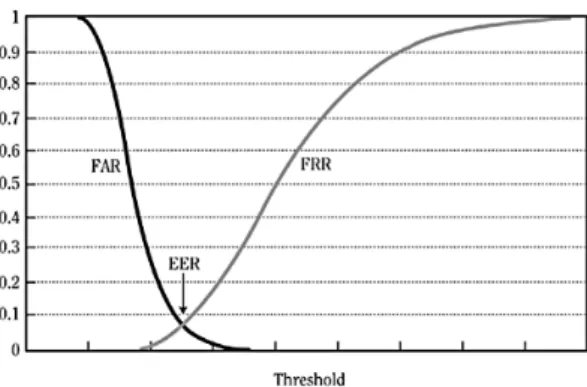
As decreasing FAR usually results in a higher FRR and vice versa, a trade-off has to be chosen between those metrics depending on the circumstances of the planned use case (Li et al., 2018, p. 32560). The EER is used to make this trade-off comparable to a certain extent: It is the value where FAR equals FRR (Figure 2.1). A lower EER indicates a more reliable system. Table 2.1 shows EERs for various biometric features as a reference.

The EER cannot be measured directly. Instead, it can be approximated by searching the classification threshold t that minimizes |FAR−FRR| and then calculating

EER= FFR+₂FRR for this thresholdt.

2_{Also called False Match Rate (FMR; Jain et al., 2004, p. 6).} 3_{Also called False Non Match Rate (FNMR; Jain et al., 2004, p. 6).}

(17)

Fig. 2.1.:EER as trade-off between FAR and FRR. Source: Reid (2004, p. 150).

Tab. 2.1.:EERs reached with biometric features. Source: Dasgupta et al. (2017, pp. 48–60). Biometric Modality EER

Fingerprint 2% Gait 7.3% Keystroke 1.8% Retina 0.8% Voice 6%

2.2

Sensors

Before working with smartphone sensor data, it is useful to know how those sensors work, what exactly they measure, and which of their characteristics possibly influence the usage of their data for analysis purposes. While smartphones contain multiple types of sensors, which also vary between vendors and models, this section is limited to cover three types that are used in the later implementation (see Chapter 5).

2.2.1

Accelerometer

Accelerometers measure the acceleration a, which is described as the change in velocity dv over timetdivided by time of the velocity changedt. As the velocity

v can also be described as the derivation of distancex over timet, acan also be described by using the change in distance. (Hering and Schönfelder, 2018, p. 371)

a(t) = dv(t)

dt =

d2x(t)

dt2 (2.3)

That’s how the acceleration can be derived from measuring the time and deflection of a springy mounted mass during the exposure to an accelerating force (Figure 2.2).

(18)

Sensors in smartphones are built as Microelectromechanical Systems (MEMSs) and detect the position of a mass mounted in a substrate by measuring electric capacity (Figure 2.3) (Hering and Schönfelder, 2018, pp. 372f). A single accelerometer can measure the linear acceleration along a single axis. Therefore, three of such devices are needed to cover the three-dimensional space.

From the output of the accelerometer, the velocity v is calculated by integrating accelerationawhile the positionxcan be derived from integrating velocity (W3C, 2019, Sec. 3.1): v= Z a·dt and x= Z v·dt (2.4)

Therefore, it is theoretically possible to obtain the orientation of the accelerometer in space. But the double integral amplifies the sensors drift (see Section 2.2.5) and renders the positionxtoo imprecise for most applications. (W3C, 2019, Sec. 3.1)

2.2.2

Gyroscope

Gyroscopes are devices to measure angular displacement per time or so-called angular velocity. A single gyroscope can detect the angular rate against one axis. Therefore, three gyroscopes need to be combined to cover all three axes of space (Hering and Schönfelder, 2018, pp. 374f.). For sensors in modern smartphones, three so-called Coriolis Vibratory Gyroscopes (CVGs) are combined in a single MEMS (Kalantar-zadeh, 2013, pp. 143–145).

The gyroscopes that are embedded in consumer devices like smartphones are usually based on a vibrating mass (Figure 2.4). This mass vibrates along one axis and gets deflected by the Coriolis force when it is exposed to a torque. The sensed deflection is used to calculate the angular velocity of the movement. Because of the constant high-frequency vibration, gyroscopes are among the sensors with the highest power consumption. (W3C, 2019, Sec. 3.2) F=D_⋅v F=K_⋅x F=m_⋅a x Spring Damping Mass

(19)

+

−

Electrodes Electrodes Substrate Case with Electrodes Test Mass

+ + + + +

−

− − − −

Fig. 2.3.:Schematic of a capacity based MEMS accelerometer. Source: Hering and Schön-felder (2018, p. 373).

Fig. 2.4.:Schematic of a vibrating gyroscope. Source: Kalantar-zadeh (2013, p. 145).

The angular velocitywcan be used to calculate the angular distance moved during the time spandt, which could then be used to determine the current angleθof the gyroscope itself (W3C, 2019, Sec. 3.2):

θnn=θn−1+w·dt (2.5)

But like with accelerometer drift generated by noise has to be considered.

2.2.3

Magnetometer

While there are different types of magnetometers available, the most common types used in today’s smartphones are based on Anisotropic Magnetoresistance (AMR) or Giant Magnetoresistance (GMR). Those types can be miniaturized, show a low power consumption as well as low production costs. But they still provide a magnetic resolution in the order of 1–10 nT which is good enough for navigation purposes on Earth5. (Vˇcelák et al., 2015, pp. 1077f)

AMR and GMR are Magnetoresistance (MR) effects: if a conductor of a particular material gets exposed to a changing external magnetic field its electric resistance changes. This change in resistance can be measured and used to infer the strength of the external magnetic field. Both AMR and GMR are effects appearing in

ferromag-5_{The magnetic field of the Earth ranges between 25,000 and 65,000 nT depending mostly on the}

location of measurement. (Wikipedia contributors, 2018)

(20)

Fig. 2.5.:Bosch SensorTech BMI263 IMU. Source: Bosch Sensortec (2018a).

netic materials. AMR-based magnetometers are cheaper to produce than GMR-based magnetometers, which on the other hand are smaller, more accurate and have a lower power consumption. (Hering and Schönfelder, 2018, pp. 13–16)

Similar to accelerometer and gyroscope, a magnetometer in a smartphone needs to measure the strength of the magnetic field on all three axes to cope with different possible orientations of the phone (Vˇcelák et al., 2015, pp. 1077f). To determine the direction in which the device is pointing the gravity vector, detected by the accelerometer and optionally gyroscope, is needed. (W3C, 2019, Sec. 3.3)

2.2.4

IMU

A three-axis accelerometer and a three-axis gyroscope can be combined in a single chip, sometimes also including a three-axis magnetometer. Such an Inertial Measure-ment Unit (IMU) can be produced as small as a gyroscope or accelerometer alone. An example of such a device is the BMI263 by Bosch SensorTec (Figure 2.5). This Inertial Measurement Unit (IMU) covers flexible measurement ranges which can cover from 125 °/s up to 2000 °/s of angular rate for the accelerometer and from 2 g up to 16 g for the gyroscope with a digital resolution of 16 bit. One benefit of IMUs like the BMI263 over the standalone sensors is the possibility to include self-calibration features. Some applications for such a device are image stabilization, panorama panning, or gesture recognition. (Bosch Sensortec, 2018b)

2.2.5

Constraints regarding Sensor Data

While the quality of the sensor output generally increases with the development of new smartphone generations, the data quality will keep competing with other factors like production costs, size, and energy consumption. As those compromises affect the data quality and analysis, it’s useful to know their possible consequences, which influences their impact and how they can be compensated.

(21)

One unwanted effect is the so-called “noise”: Random fluctuations appearing in the output signal of the sensors, even if the measurand doesn’t change. The signal-to-noise ratio is a standard metric to describe its influence and is calculated by dividing the mean of the sensor’s signal by the standard deviation of the noise (Kalantar-zadeh, 2013, p. 14). A gradual change in the sensor’s output occurring even if the measurand stays constant is called “drift”. It is a systematic error and manifests itself in a change of the sensor’s baseline, i.e. the output value that the sensor generates without any stimulus (Kalantar-zadeh, 2013, p. 16). Inaccuracies during calibrating the sensors can lead to a so-called “calibration error”, which systematically shifts the signal’s output away from the input value of the stimulus (Fraden, 2016, p. 42). Multiple internal and external factors influence noise, drift, and calibration errors. They can even vary between the same sensors of the same batch. Some external factors are temperature, electromagnetic signals, or mechanical vibrations (Kalantar-zadeh, 2013, p. 14). E.g., the magnetometer experiences an offset drift depending on the temperature of the sensor. Hard or soft magnetic material in the surrounding of the sensor can produce magnetic disturbances as well (Vˇcelák et al., 2015, p. 1078). Even the intensity of the Earth’s magnetic field itself changes significantly depending on the distance to the poles. Temperature changes are also known to cause electronic noise (Kalantar-zadeh, 2013, p. 14). Errors from internal factors can be rooted in construction, production, assembling, or calibration. They can slowly appear over time, e.g., through the degeneration of the sensor’s material, which is known to influence the drift of sensors (Kalantar-zadeh, 2013, p. 14).

Some of the mentioned constraints can be reduced by fusing data from multiple sensors into a so-called high-level sensor. E.g., an absolute orientation sensor can be implemented by leveraging the gravitational vector detected by the accelerometer and the vector pointing to the North detected by the magnetometer. Additionally, data from the gyroscope can be used to enhance those vectors. Such a high-level sensor can provide orientation information stationary to the Earth’s plane like it is needed for Augmented Reality applications (Figure 2.6). Such high-level sensors often include preprocessing of the data, like removing noise with low-pass and high-pass filters and also are available as MEMS. (W3C, 2019, Sec. 4)

(22)

-X +Z -Z -Y +Y uB uE uN uG +X N W Y X Z

Fig. 2.6.:Smartphone’s absolute orientation: Gravity vectoruGfrom accelerometer and magnetic field vectoruB from magnetometer are used to calculate the vectors uEpointing to East (uE =uB×uG) and vectoruN pointing to North (uN =

(23)

3

Related Work

This chapter presents related work to this thesis in a cross-sectional manner by comparing different methods chosen in previous studies for each step in the machine learning process. That deviates from common practice to present related work by sequentially describing studies one after the other. The intention behind this structure is to provide a better overview of the possible options for the individual steps as a foundation for the choices to make during the implementation. The downside of this structure is that the decisions made by the different authors are taken slightly out of context. Please refer to the original papers to get the full picture of the individual approaches.

Table 3.1 shows an overview of studies closely related to this thesis, which means, they are investigating CA using only smartphones’ sensor data, leveraging at least one inertial sensor and relying on regular6smartphone usage. Related studies that do not quite match these criteria but are regularly referenced in the field of CA are listed in Appendix A.1. It is important to note that the experimental setups of the different studies differ regarding various important aspects, like the used datasets, the usage of different sensors (between 1 and 30 different sensor modalities) and differences in the evaluated attack scenarios. Due to those differences, the performance metrics reported in the table are not directly comparable!

3.1

Datasets

Even though there are multiple public datasets available containing smartphone sensor data for the purpose of activity recognition7those are usually not useful for CA, because the datasets were recorded in very controlled environments, with fixed mounted smartphones or published without subject information. One exception is the “Complex Human Activities Dataset (CHAD)” (Shoaib et al., 2016) as a collection focused on activity recognition, which also has been used for CA by E.-u.-Haq et al. (2017). It is limited to 10 subjects performing predefined activities for about 3–5 min

and are thus not comparable to a real-world scenario.

6_{The user doesn’t have to adjust his behavior or perform additional actions for the authentication.} 7_{E.g. “Smartphone-Based Recognition of Human Activities and Postural Transitions Data Set”}

(Reyes-Ortiz et al., 2015) or “WISDM Activity Prediction” (WISDM Lab, 2012).

(24)

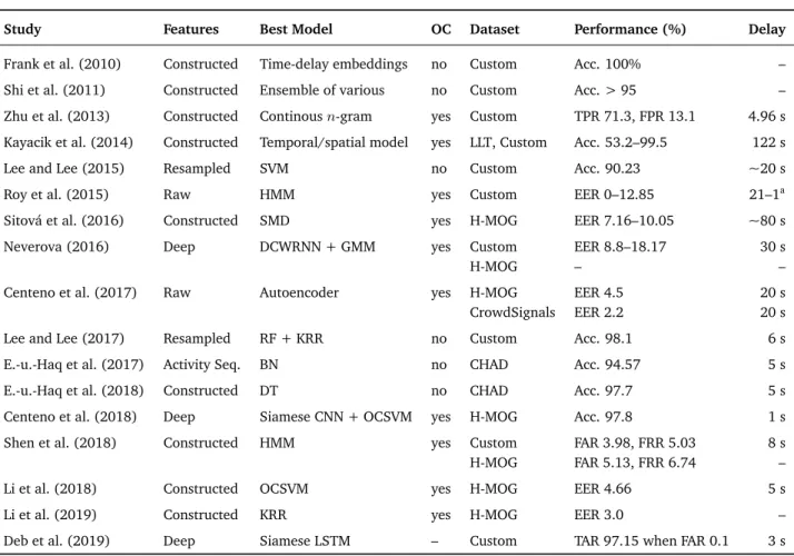
Tab. 3.1.:Key-Studies in the field of CA using mobile phone sensors, ordered by year of publication. Column “One Class” (OC) indicates if only owner data is used during the final classification. The metrics for performance and detection delay are listed as reported by the authors.

Study Features Best Model OC Dataset Performance (%) Delay

Frank et al. (2010) Constructed Time-delay embeddings no Custom Acc. 100% – Shi et al. (2011) Constructed Ensemble of various no Custom Acc. > 95 – Zhu et al. (2013) Constructed Continousn-gram yes Custom TPR 71.3, FPR 13.1 4.96 s Kayacik et al. (2014) Constructed Temporal/spatial model yes LLT, Custom Acc. 53.2–99.5 122 s

Lee and Lee (2015) Resampled SVM no Custom Acc. 90.23 ~20 s

Roy et al. (2015) Raw HMM yes Custom EER 0–12.85 21–1a

Sitová et al. (2016) Constructed SMD yes H-MOG EER 7.16–10.05 ~80 s

Neverova (2016) Deep DCWRNN + GMM yes Custom EER 8.8–18.17 30 s

H-MOG – –

Centeno et al. (2017) Raw Autoencoder yes H-MOG EER 4.5 20 s

CrowdSignals EER 2.2 20 s

Lee and Lee (2017) Resampled RF + KRR no Custom Acc. 98.1 6 s

E.-u.-Haq et al. (2017) Activity Seq. BN no CHAD Acc. 94.57 5 s

E.-u.-Haq et al. (2018) Constructed DT no CHAD Acc. 97.7 5 s

Centeno et al. (2018) Deep Siamese CNN + OCSVM yes H-MOG Acc. 97.8 1 s

Shen et al. (2018) Constructed HMM yes Custom FAR 3.98, FRR 5.03 8 s

H-MOG FAR 5.13, FRR 6.74 –

Li et al. (2018) Constructed OCSVM yes H-MOG EER 4.66 5 s

Li et al. (2019) Constructed KRR yes H-MOG EER 3.0 –

Deb et al. (2019) Deep Siamese LSTM – Custom TAR 97.15 when FAR 0.1 3 s a_{number of touch actions}

The dataset “LiveLab Traces (LLT)” (Shepard et al., 2011) consists of smartphone data from 35 users and includes multiple sensor modalities besides the inertial sensors, like app usage and call information. On the downside, the duration of the data captured per user strongly varies from a few days to close to a year.

Another ambitious project called “CrowdSignals” tried to collect a vast amount of smartphone sensor data for multipurpose analytical use cases. But after their crowdfunding succeeded, they only published a small dataset sample until today (AlgoSnap Inc., 2015). However, at least Centeno et al. (2017, p. 5) achieved to get early access to the dataset for their research.

To my best knowledge, until now, there is only one publicly available dataset specifically for CA, which was collected by Yang et al. (2014b). It’s commonly referred to as the “Hand Movement, Orientation and Grasp (H-MOG)” dataset and consists of data by inertial and touch sensors and was produced by 100 subjects during 24 sessions. In those sessions, the users had to perform predefined activities

(25)

mirroring realistic scenarios. While the dataset is of good quality, two aspects are limiting its usefulness for the use case of this thesis: All sessions include active usage of the smartphone, and they are of a pretty short duration of 5–15 min. The dataset became quasi-standard because of its public availability, proper documentation and ease of use. It was leveraged by various researchers, as a primary dataset by Sitová et al. (2016), Centeno et al. (2017), Centeno et al. (2018), Li et al. (2018), and Li et al. (2018) or for benchmarking of different approaches by Shen et al. (2018). Other researchers like Roy et al. (2015), Neverova (2016), Shen et al. (2018), and Deb et al. (2019) undertook the effort to collect custom datasets but did not publish them. Outstanding in the aspect of scale is the collection of Neverova (2016, pp. 179f) which was performed by Google as part of a project called “Abacus”8: It is reported to include data from approximately 1500 users captured in real life situation. The dataset with probably the most features was collected by Deb et al. (2019, pp. 3f) and is supposed to include 30 different sensor modalities captured in

a real-world setting.

3.2

Data Preprocessing

The input data for machine learning algorithms must be provided in an adequate amount, structure, and format for the particular task. Data preprocessing comprises of a set of techniques to transform raw data into the desired form. The decisions to be made during this process strongly influence the performance and characteristics of the final model. (García et al., 2015, p. 10)

The steps performed during data preprocessing depend on the characteristics of the raw data, the targeted machine learning model, and its use case specific application. It is not surprising that the studies related to CA using smartphone data applied quite different techniques during this process. The following section summarizes relevant approaches. If not explicitly stated otherwise, the studies do not provide clear information about the impact of those specific steps. This section is meant as an overview of options and doesn’t conclude any recommendation.

3.2.1

Noise Filtering

During the process of collection, it is unavoidable that the data gets contaminated by imperfections to a certain degree. This kind of noise affects the performance and robustness of the machine learning models trained with this data. Noise filtering

8_{The project “Abacus” was guided by Google Inc. to eliminate the necessity of protecting smartphone}

applications with passwords. (Neverova, 2016, pp. 6f)

(26)

denotes a set of techniques used to improve data quality before feeding it to the model for training. (García et al., 2015, pp. 107f)

To reduce noise in the sensor’s signal (see Section 2.2.5), E.-u.-Haq et al. (2018, p. 27) applied a smoothing filter with a length of 3 samples at 50 Hz frequency, while Deb et al. (2019, p. 5) leveraged Fast Fourier Transform (FFT) to handle and remove noise by mapping the measurements of the movement sensors from time domain to frequency domain.

Shen et al. (2018, p. 51) propose a process called “kinematic information extraction” composed of two steps for filtering data of inertial sensors and touch events. First, the gravity component of the accelerometer’s signal is removed by employing a Kalman filter under the assumption that the device’s acceleration without distortion by gravity reflects the motion of the smartphone more accurately. In a second step, noise reduction is performed by decomposing the signals using wavelet functions, applying threshold analysis to the components, and afterward reconstructing the original signal by using the inverse wavelet functions. This approach acknowledges that signal noise appears at the whole spectrum of frequencies of the signal sensor. Reyes-Ortiz et al. (2015) also separated the gravitational and movement components from the acceleration signal but decided to use a Butterworth low-pass filter with 0.3 Hz cutoff frequency to target the assumed low frequencies of the gravitation.

3.2.2

Manual Feature Construction

Feature construction is the application of a set of operations to a set of existing features to generate new features. Whereby those new features do not yield any new information, but might describe the existing information in a form that is more suitable for specific models or applications (García et al., 2015, p. 189). This step was applied in the majority of the examined studies “manually”: the transforming operations where chosen cognitively by the researchers.

It is common to compute features by applying a sliding window and calculating various metrics for analysis of time series like sensor data. The set of aggregation functions used for CA have already been widely tested in related fields like activity recognition (E.-u.-Haq et al., 2018, p. 28). From the commonly computed features (see Appendix A.2), the following have been reported to be quite useful for the task of CA: energy9, entropy, minimum, maximum and mean of gyroscope as well as energy and entropy of accelerometer. (Shen et al., 2018, pp. 52f)

(27)

The window parameters used for the aggregation range from 0.5 s to 5 s for window size, the step-size from 50% overlap to no overlap (E.-u.-Haq et al., 2018, p. 28; Reyes-Ortiz et al., 2015).

Beside fixed window parameters also cycle-based approaches have been evaluated. Here the features are aggregated from cycle to cycle, e.g., from step to step during gait. This cycle based approach performed weaker than the segment based procedure with fixed window parameters. The main difficulty seems to be inaccurate cycle detection in real-world environments, e.g., if the smartphone is not fixed to the body but is held loosely in hand or pocket. (Al-Naffakh et al., 2018, p. 17)

Li et al. (2018) and Li et al. (2019) transferred “data augmentation” strategies known from image classification to construct additional features by applying permutation, sampling, scaling, cropping and jittering to the samples of a particular window length. They report promising results on the H-MOG dataset (Li et al., 2018, pp. 5f). To me, the study does not clarify if this approach basically optimizes the classification for the given dataset or if it generalizes well enough to be used in a real-world scenario.

Even more advanced strategies were applied by Sitová et al. (2016, pp. 878–880), who crafted the H-MOG features, a set of metrics designed to capture grasp resis-tance and grasp stability during a touch event, and combined them with features representing tap and keystroke actions.

3.2.3

Data Reduction

It is common to reduce the number of features and instances used as model input to lower the computational effort, while maintaining a large amount of distinctive information of the original data. This process is also known as “dimension reduction” and regularly performed by grouping multiple features or selecting a meaningful subset of features. Equivalent methods performed on the instances are categorized as techniques for “data sampling”. (García et al., 2015, pp. 147f)

Shen et al. (2018) reduced their feature space from 192 features to 38 by calculating the Mutual Information (MI) score and the Fisher score regarding the class variable and applying a threshold to discard features with MI score below 0.5. They identified the energy and the entropy of the gyroscope’s signal as the most informative features. Kurtosis, skewness, and cross-mean rate resulted in MI scores below 0.5 for all sensors. Besides, Shen et al. (2018, pp. 51f) drastically reduced the number of samples by analyzing only the sensor data generated during touch events.

(28)

Al-Naffakh et al. (2018, pp. 20–22) proposed a “dynamic feature vector” and in-dividually selected a particular subset of features for every owner. As selection criteria the means of every feature of the owner have been compared to the means of every individual impostor. The more often the feature’s mean of the owner differs from the feature’s mean of an impostor by at least standard deviation, the more the feature is considered to be helpful. After this scoring, the most useful features were selected, with the best results between 30 and 80 features. From my point of view, this approach seems to be kind of simplified Gaussian Mixture Model (GMM). Neverova (2016, p. 182) used the well-known Principal Component Analysis (PCA) to transform the features into lower-dimensional space while preserving as much variation in the data as possible. Sitová et al. (2016, pp. 881f) also applied PCA but with the primary purpose of removing possible correlation between the features as a precondition for their classifiers.

3.2.4

Deep Features

A different approach that aims to reduce the number of manual steps and decisions needed for data preprocessing is to leverage ANNs to transform raw data into a meaningful representation with lower dimensionality. The ANNs are supposed to learn functions equivalent to techniques like filtering, manual feature construction, and dimensionality reduction during their training. The main downsides of this approach are the difficulty in identifying the best network architecture, the low interpretability of the learned transformation functions and often the need of a large amount of data plus compute power for training.

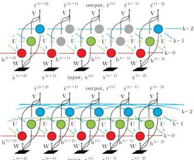
Neverova (2016, pp. 175ff) compared several network architectures regarding their ability to learn deep features in the context of Continuous Authentication (CA): CNN, vanilla Recurrent Neural Network (RNN), Long Short-Term Memory (LSTM), and Clockwork Recurrent Neural Network (CWRNN). She also proposed a new architecture named Dense Clockwork Recurrent Neural Network (DCWRNN) (Figure 3.1).

The DCWRNN is a modification of the CWRNN, which captures patterns within different temporal scales (“slower” and “faster” patterns) by partitioning the units of the hidden recurrent layers in different groups with different update frequency, the so-called frequency bands. In the original CWRNN, different subsets of units in the low-frequency bands are active over time. That slows down the learning process and results in possibly different responses to the same input at different times during testing. The DCWRNN compensates these shortcomings by introducing parallel threads shifted with respect to each other. (Neverova, 2016, pp. 176–179)

(29)

input , x( t ) _x( t + 1) x( t−1) _x( t + 2) x( t−2) V V V V V k= 0 k= 1 k= 2 h( t−1) _h( t ) _h( t + 1) W W W W W U U U U U U h( t + 2) h( t−2) ˜ y( t + 1) out put , ˜y( t ) ˜ y( t−1) ˜ y( t−2) _y_˜( t + 2) input , x( t ) _x( t + 1) x( t−1) _x( t + 2) x( t−2) V V V V V k= 0 k= 1 h( t−1) _h( t ) _h( t + 1) W W W W W U U U U U h( t + 2) h( t−2) ˜ y( t + 1) out put , ˜y( t ) ˜ y( t−1) ˜ y( t−2) _˜_y( t + 2) k= 2 U

Fig. 3.1.:Comparison of the original Clockwork RNN (top) with its sometimes inactive units (grey) in the lower frequency bands (green, blue) and its modification called Dense Clockwork RNN (bottom). Source: Neverova (2016, p. 177).

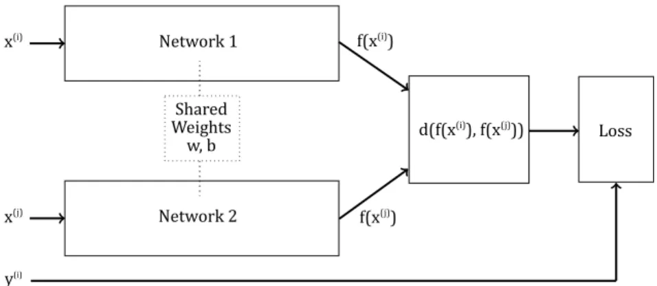
Centeno et al. (2018, pp. 3f) used a different network architecture. They trained a Siamese CNN to learn features representing the difference in raw sensor data between the owner and impostors. During authentication, this model computes deep features, which are then fed into an OCSVM. This approach was reimplemented as part of this thesis and is described in detail in Section 4.5.2.

During the writing of this thesis, Deb et al. (2019, p. 5) published another variant: They claim to improve the quality of deep features generated by the Siamese network by using LSTMs instead CNNs for the two sub-networks (Figure 3.2).

Fig. 3.2.:Architecture of Siamese LSTM. Source: Deb et al. (2019, p. 5).

(30)

3.2.5

Context Information

All the studies that evaluated the authentication performance of their models regard-ing different user contexts (e.g. “sittregard-ing”, “standregard-ing”, “walkregard-ing”) revealed significant varying performance of the same model in different settings. E.g., models tend to perform better when the user is walking compared to when he is sitting.10

Therefore, it is possible to take circumstances into account by detecting the user’s context and using different authentication models for those different situations. Lee and Lee (2017, p. 304) tried classifying the samples into four different contexts first but ended up using two different context models in the end. E.-u.-Haq et al. (2017, p. 206) differentiated between six activities but provide classification metrics only for the final authentication model and not for the context classification itself.

3.3

Classifiers

The main task during CA is to classify the incoming sensor data of the device as produced by the owner (positive class) or as produced by an impostor (negative class). In related studies, this problem was either interpreted as a binary classification problem or as a problem of novelty detection, whereas only data of the positive class is used during classifiers’ training. Consequently, classifiers based on those two types of machine learning algorithms have been evaluated. This section provides an overview of models which are considered to be most relevant.

3.3.1

Gaussian Mixture Model

Gaussian Mixture Model (GMM) is a generative probabilistic algorithm to model input data as a mixture of multi-dimensional Gaussian probability distributions and can be used similar tok-Means as clustering algorithm (VanderPlas, 2016, pp. 476f). As a consequence, it can also be used to represent the feature density of each class and predict probabilities of membership to these classes for an input vector. This enables the use of GMM for classification tasks (Hastie et al., 2009, p. 463).

One aspect that makes GMM interesting for CA is the possibility to train a so-called Universal Background Model (UBM) first using an iterative Expectation-Maximization algorithm on all data and to later adapt this more generic model to new training data by retraining it using Maximum A Posteriori estimation (Reynolds,

10_{Shen et al. (2018, p. 55) reported the only exception and presented better results during sitting than}

walking, but the Hidden Markov Model (HMM) used in this study also is quite different from the other approaches.

(31)

2009). Hence, it’s possible to do a compute-expensive pretraining of the GMM centrally with data from all subjects included in the training dataset, then distribute the UBM to the individual smartphones where it can be updated with the owner’s data, which doesn’t even have to be included in the central training dataset. Neverova (2016, p. 173) leverage this approach by pretraining the GMM on a large amount of data with deep-features generated by their DCWRNN (see Section 3.2.4), then retraining this generic UBM individually for every user and combining both UBM and individualized user model as an ensemble classifier.

3.3.2

One Class Support Vector Machine

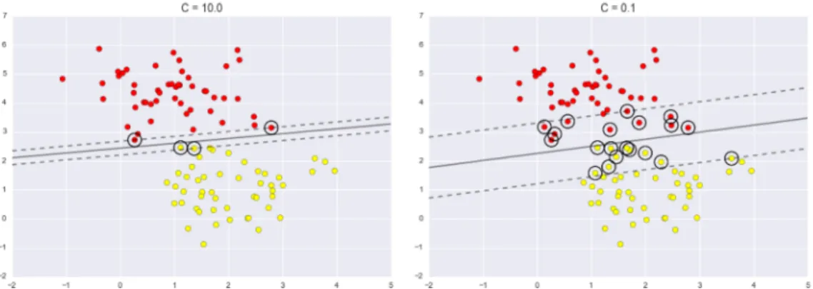
OCSVMs are a variant of the well-known Support Vector Machines (SVMs), a class of linear algorithms leveraged for solving e.g., classification or regression problems (Zhang, 2017). OCSVMs are trained with data limited to a single class to perform Novelty Detection on the testing data. As OCSVM is one of the models used for this thesis, it is described in more detail as part of the concept chapter in Section 4.5. Sitová et al. (2016, p. 880) tested an OCSVM with Radial Basis Function (RBF) Kernel against two other single class models, Scaled Euclidean Distance (SED) and Scaled Manhattan Distance (SMD). They report OCSVM to result in the highest and therefore worst EER, but with the remark that the performance of the three models was close to par for walking scenarios and only strongly deviating in sitting situations (Sitová et al., 2016, p. 882). Shen et al. (2018, p. 54) used an OCSVM with an RBF Kernel as one of their baseline models and reported worse results compared to their main Hidden Markov Model (HMM). Centeno et al. (2018, p. 5) leveraged the OCSVM with an RBF Kernel as their only authentication model.

Lee and Lee (2015, pp. 5f) used a standard SVM as their only authentication model first, but later tested it against Kernel Ridge Regression (KRR), a Naive Bayes classifier, and a Linear Regression. The SVM was almost as good as the best performing KRR model regarding the classification results but was rejected in favor of KRR because of SVM’s higher computational needs (Lee and Lee, 2017, pp. 302f). In the study by E.-u.-Haq et al. (2018, p. 31), the SVM performed better than the competing models k-Nearest Neighbors (k-NN) and Decision Tree (DT).

3.3.3

Hidden Markov Model

Roy et al. (2015) was among the first employing Hidden Markov Models (HMMs) for CA using smartphone sensor data. The underlying idea is that subsequent user

(32)

interactions can be interpreted as states in a Markov Process, where a stochastic function can represent the transitions between different states. Such HMMs can be used as a one class classifier and trained with only data from the owner. Roy et al. (2015) analyzed user interactions with their smartphones and identified the two most common touch gesture types: slide and tap gestures. For those they build two separate classifiers, each consisting of three HMMs, one for each data source: “touch”, “vibration” and “rotation”. The likelihood scores of the classifiers are averaged to get a combined score. That ensures robust results, even if data from a single sensor is unavailable for a certain time. When classifying multiple subsequent gestures, their mean in a specific window is used as the authentication score to provide more robust results. (Roy et al., 2015, pp. 1311–1313)

Shen et al. (2018) implemented a similar HMM based classifier. By using a larger pool of subjects from their own data collection, they claim to have been able to extract more informative behavioral features and improved the results of the classifier to an EER between 4.74% and 9.73% depending on the usage scenario.

Quite refreshing in the study by Shen et al. (2018) is their extensive evaluation. E.g., they discovered, that EER seems to decrease when the amount of training data gets too big: They tested short-, medium-, and long-term scenarios with mean training events of 154, 201 and 624, and reported EERs of 6.23%, 4.03% and 8.11%. Shen et al. (2018) suspect the longer time span between training and testing events as a reason for this observation. During the evaluation, the HMM based classifier revealed better results than a competing SVM and an ANN model. The authors argued the HMM captures the temporal nature of the sequence of events better than the other models. (Shen et al., 2018, pp. 56f)

3.3.4

Artificial Neural Networks

Besides being leveraged to generate deep features (see Section 3.2.4), ANNs were also studied as classifiers during authentication. Shen et al. (2018, pp. 54f) tested a three-layered Multilayer Perceptron (MLP) as comparative model against their main HMM classifier as well as against an OCSVM. The architecture consists ofninput nodes for nfeatures,n·2nodes in a single hidden layer and a single node in the output layer. This node’s output is then used as the classification score. The neural network performed worst for all tested scenarios. However, the publication misses information on how exactly the MLP was trained in a one class approach.

Centeno et al. (2017) studied the use of an autoencoder as authentication classifier. They presented very promising results, but there are some open questions regarding the implementation, which I want to describe in the following in more detail.

(33)

In general, an autoencoder is a type of Artificial Neural Network (ANN) that is unsupervised trained to first encode a given vector from the input layer into a representation, the so-called code, which is described by a hidden layer of the network, and afterward, reconstruct the input from the code. The reconstruction is served in the output layer. It would not be especially useful if the autoencoder would be able to reconstruct the input vector exactly. Therefore, some restrictions are set upon the network which forces the autoencoder to approximate and only learn those aspects of the input data, which are most useful to reconstruct input vectors as good as possible. For some applications of autoencoders, the ability to reconstruct is only a means to an end for learning to generate the code, which can be leveraged for feature learning or dimensionality reduction. (Goodfellow et al., 2016, p. 499) For an overview of the different autoencoder variants, I recommend Goodfellow et al. (2016, Chapter 14), while Hinton and Salakhutdinov (2006) describe the under-complete autoencoder in more detail.

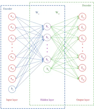
The variant of autoencoder, that Centeno et al. (2017, p. 4) leveraged for smartphone-based CA, is the under-complete autoencoder (Figure 3.3). In this architecture, the hidden layer representing the code has smaller dimensions than the input data and thereby forces the autoencoder to learn a useful representation. During the learning process, a loss function, which describes the dissimilarity between the input vector and its reconstruction, is minimized. (Goodfellow et al., 2016, pp. 500f)

Centeno et al. (2017, p. 4) trained the autoencoder with samples from the owner in a single class approach. The idea is that the network learns to reconstruct the data from the user, which it was trained on, better than the data from unknown users. The distance between the input vector and its reconstruction is expected to be lower for samples from the owner, than for a sample from an impostor. The samples are classified binary by applying a threshold on this distance.

One aspect in the given implementation surprised me: Centeno et al. (2017, p. 6) used 1500 units in each hidden layer (they tested three setups using one, three, and five hidden layers). As they took 500 samples as input vector, and each sample consists of three values for each axis of the accelerometer, it means that the autoen-coder actually was not set up as an under-complete autoenautoen-coder like depicted in their architecture chart (Figure 3.3). Also, no other kind of regularization like the sparse penalty is mentioned but would be expected for such an architecture. Via correspondence11I learned that different numbers of hidden units have been tested (e.g.,1500×750×350×750×1500) but ended in similar results which was also

surprising to hear.

11_{E-Mail by M. P. Centeno, 26th Feb. 2019.}

(34)

Fig. 3.3.:Autoencoder architecture with one hidden layer. ax1, ay1, az1 . . . axn, ayn, azn

are a set of accelerometer measurements taken as input,h1 . . . hnare activation

functions generating the code.W andbdenote weights, and bias vectors learned by the encoder and decoder sections. Source: Centeno et al. (2017, p. 4).

3.4

Evaluation Settings

An aspect that came to my attention during the review of related studies is the absence of any kind of standardized approach for evaluating the performance of the models in the context of CA. The different evaluation settings used by the authors prevent any meaningful comparison between the studies. It is concerning that this situation does not stop most authors from comparing the metrics directly. This section describes aspects of the evaluation which are considered to be most relevant and tend to be handled differently in the various studies.

One of the issues which make direct comparison impossible is that the studies use different metrics to report the performance of their approaches (s. Table 3.1). The Equal Error Rate (EER), one of the standard metrics for the biometric authentication system (see Section 2.1.4), is reported as a metric by roughly one-third of the stud-ies. Nearly half of the studies report accuracy (number of correctly classified objects

divided by total number of objects) as the classification metric. Even if this metric is applied to balanced datasets12, it doesn’t reveal if the model has weaknesses regarding false positives or false negatives, which has important implications for authentication use cases. Most studies provide at least Receiver Operating

Character-12_{For datasets with unbalanced classes, accuracy is significantly harder to interpret and compare. If}

in such cases the class distribution is not reported along with the accuracy, the metric becomes meaningless.

(35)

istic (ROC) plots to give these insights. A minority of studies reported only FAR and FRR as their primary metrics. As those metrics are parts of a trade-off, it needs a justification for reporting specific values. None of the affected studies explicitly states such an explanation, but at least they all provide plots comparing FAR and FRR. Those plots suggest that the reported values maybe were selected using elbow-points. Deb et al. (2019, pp. 7f) reported the True Acceptance Rates (TARs) corresponding with FAR 1% and 0.1% without stating reasons for those thresholds.

Another problem iswhatis reported as the final authentication metric. E.g., Deb et al. (2019) present metrics for the ability of their Siamese LSTM to distinguish positive

pairs and negative pairs as “authentication performance”, but without stating how the classification was done.13 _{It is also unclear to me how this approach should} be implemented in a real authentication situation, especially how the positive and negative pairs should be generated in such a case, and if the results would be comparable. E.g. Deb et al. (2019, p. 6) compared their metrics with the metrics reported by Centeno et al. (2018), but they both were derived quite differently: Deb et al. (2019) reported the outcome of classifying positive and negative pairs with their Siamese LSTM, while Centeno et al. (2018) used the Siamese CNN to generate deep features as an input for a subsequent OCSVM and reported the final authentication metrics. In my opinion, Deb et al. (2019) compares metrics of a binary classification approach with metrics of a more difficult one class approach.

Some studies distinguish the performance regarding different usage scenarios like walking or sitting, and report the metrics separately (Sitová et al., 2016, p. 877; Shen et al., 2018, pp. 55f), while others report overall results (Centeno et al., 2017, pp. 7f; Li et al., 2018, p. 11).

As a third problem, the evaluation setup varies a lot between the studies. Centeno et al. (2017, p. 7) report the average of cross-validating 10 random “attack scenarios”, where such a scenario is defined as classifying testing samples from the owner, whose data was used to train the model, against the same number of samples from another randomly selected user (1 vs. 1). On the other hand, Li et al. (2018, p. 6) classified a certain amount of the owner’s samples along with the same amount of samples randomly drawn from all 98 other users’ data (1 vs. all). Additionally, while most studies reported the metrics for classifying a single sample, others like Shen et al. (2018, p. 54) and Roy et al. (2015, p. 1313) report a “robust” value, which improves

accuracy by calculating the mean of the individual sample’s score across a sliding window. Those different approaches are valid and justified, but make the results harder to compare.

13_{One possibility would be a threshold on the Euclidean distance between the deep features. Another}

would be an additional single node layer in the network using the deep features as input.

(36)

Finally, different datasets contribute to the difficulty of comparison. At least Shen et al. (2018) and Centeno et al. (2017) report results using the H-MOG dataset as a reference along with a second dataset. But due to limitations of the dataset, this is not always possible, e.g. Neverova et al. (2016, p. 1815) stated, H-MOG is too small for their approach, other studies like Deb et al. (2019, p. 2) leveraged sensor data that is not included in H-MOG. To my best knowledge, Sitová et al. (2016) (the authors of H-MOG) were the only researchers to publish their datasets. Therefore, all other studies with custom datasets are not reproducible.

As described above, the direct comparison of the various studies’ results is difficult. Therefore, it is important to value the contributions of Khan et al. (2014) and Shen et al. (2018) who are so far the only ones to provide comparative studies for the different approaches. Khan et al. (2014) reimplemented six approaches published between 2010 and 2014, including three approaches leveraging inertial sensors. They evaluated accuracy, training delay, as well as computational complexity. Shen et al. (2018), as part of assessing their own approach, also reimplemented six different approaches published between 2013 and 2016. They used their custom dataset as well as H-MOG for the evaluation. The result of this comparative study provides a different view on the performance of the various models than the individual results reported by the different authors do. Unfortunately, Shen et al. (2018) only provide FAR and FRR as classification metrics. They also stated that their results should not be generalized, and further investigation would be needed for a realistic comparison. (Shen et al., 2018, pp. 58f)

(37)

4

Concept

This chapter describes the ideas behind the implementation of Continuous Au-thentication (CA) using smartphones’ inertial sensors presented in this thesis. It condensates the options and knowledge gained from related studies (see Chapter 3) into a coherent concept fitting to the circumstances of this thesis.

First, I describe the general idea of how to apply smartphone based CA in practical use cases. Then I justify the design decisions I made before implementation and explain the algorithms which have been identified as promising. Evaluation criteria for testing the performance of the applied models are presented as well as the evaluation setup in which those metrics should be computed to gain valid results.

4.1

General Idea

The general idea behind smartphone based CA is to estimate the probability of the current smartphone’s user being the smartphone’s owner. That idea is built upon the premise that a smartphone is typically tied to a single person, the owner, and not regularly shared among multiple persons.

In a practical use case, the authentication process would be divided into three phases: First, an enrollment phase, followed by continuous authentication and updating phases. The last phase, which is needed to keep the model up to date over a longer time-span, is not in the scope of this thesis but could look similar to the enrollment phase. I present the first two phases in the following as a generic framework, not a concrete architecture. It is designed upon an authentication framework presented by Crouse et al. (2015, p. 137).

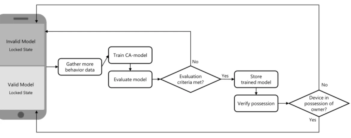
In the enrollment phase, the smartphone gathers data, which is used to train a model for authentication (Figure 4.1). This model is then evaluated, e.g., by testing it with the owner’s data and a predefined set of impostor data. If the model is considered as not good enough, more data will be gathered, and the model will be retrained and reevaluated. If the model meets the evaluation criteria, it is stored for usage in the authentication phase. But before switching to the authentication phase, it is necessary to check additional criteria like if the smartphone is still in possession of

(38)

Invalid Model Locked State Valid Model Locked State Device in possession of owner? Gather more behavior data Train CA-model No No Yes Yes CA: Continuous Authentication

Evaluate model _{criteria met?}Evaluation _{trained model}Store

Verify possession

Fig. 4.1.:Schematic of the enrollment phase of the proposed authentication framework.

Valid Model Locked State Valid Model Unlocked State System in locked state? Fallback authentication successful? Gather behavior data Classify data

(CA) Authenticationsuccessful?

Ask for password, PIN or fingerprint (KA/BA) Yes No Yes Yes No No

CA: Continuous Authentication, KA: Knowledge-based Authentication, BA: Biometrical Authentication Fig. 4.2.:Schematic of the authentication phase of the proposed authentication framework.

its legitimate owner. Otherwise, an attacker could take the smartphone during the enrollment phase, train the model with his data, and get access to the system, before the legitimate owner reports the loss of his device.

In the authentication phase, the device starts in a locked state and begins to gather data for analysis continuously (Figure 4.2). If the classification detects an appropriate certainty of the device being in possession of its legitimate owner, the authentication is considered successful and the device switches to an unlocked state. The device gets locked if the likelihood falls below a threshold. As a fallback, the user should be able to authenticate using standard methods like a PIN or two-factor authentication. The steps for the enrollment phase could be processed locally on the phone, but model training and evaluation in the cloud could be possible, too. The authentication phase should not rely on a network connection and should be processed only locally. The authenticated “locked state” does not necessarily need to correspond with the lock state of the smartphone’s operating system. It is meant more generic and can, e.g., reflect the authentication state against a third party system that communicates with the phone over network or Bluetooth.

(39)

4.2

Use Case

Different use cases for smartphone-based CA are tightly bound to the smartphone usage itself, where, e.g., login data is automatically provided to applications running on the smartphone, or where the phone is automatically locked if it is taken out of the owner’s hands.

The general use case for CA considered in this thesis, on the other hand, is focused on authentication against third-party systems unrelated to the owner’s usage of the smartphone. Such systems could be services that create an alert if a smartphone was taken from its legitimate owner, or physical access control systems like safes, which could use the presence of an authorized person as an additional authentication factor. The proof of authentication could be provided as a token over network or radio contact to the third party system performing the authorization, but this transmission is out of this thesis’ scope. Nevertheless, the differentiation between those use case types has an impact on the design decisions presented in the following section. I will reason in the following section, that the use case considered in this thesis has some different requirements than use cases that are bound to the smartphones’ usage. The targeted operational area is office space and also has an impact on the requirements. It has to be considered that the behavior of the users and their smartphone usage might differ in business situations from private situations.

4.3

Design Decisions

Some decisions strongly influence the implementation as well as the productive operation of the system. It is essential to justify the decisions transparently, as there is no clear right or wrong for choosing between the various design options.