Digital Video Forensics

(1)

Digital Video Forensics

A Thesis

Submitted to the Faculty

in partial fulfillment of the requirements for the degree of Doctor of Philosophy in Computer Science by Weihong Wang DARTMOUTH COLLEGE Hanover, New Hampshire

June, 2009

Examining Committee:

(chair) Hany Farid, Ph.D.

Devin Balkcom, Ph.D.

Fabio Pellacini, Ph.D.

Lorenzo Torresani, Ph.D.

Brian W. Pogue, Ph.D. Dean of Graduate Studies

(2)

(3)

Abstract

We present new forensic tools that are capable of detecting traces of tampering in digital video without the use of watermarks or specialized hardware. These tools operate under the assumption that video contain naturally occurring properties which are disturbed by tampering, and which can be quantified, measured, and used to expose video fakes. In this context, we offer five new forensic tools (1) Interlaced, (2) De-interlaced, (3) Double Compression, (4) Duplication, and (5) Re-projection, where each technique targets a specific statistical or geometric artifact. Combined, these tools provide a valuable first set of forensic tools for authenticating digital video.

(4)

Acknowledgments

First, I would like to thank my advisor, Hany Farid, for bringing me into the image science group. I am grateful for his patient guidance, and for teaching me the value of hard work in research. Thanks as well to the other members of my committee, Devin Balkcom, Fabio Pellacini and Lorenzo Torresani, for their comments and suggestions. I am grateful to my professors: Chris Bailey-Kellogg, Thomas Cormen, Prasad Jayanti, Chris McDonald, Doug McIlroy, Bill McKeeman and Daniel Rockmore, for all that I have learned from them. I’d also like to thank past and current members of the image science group: Siwei Lyu, Alin Popescu, Kimo Johnson, Eric Kee and Jeff Woodward. I am also grateful to the staff and system administrators for keeping everything running smoothly.

I thank my parents and my brother for their love and support all these years. Whenever I encountered difficulties, it was always their love that sustained me.

(5)

3.4 Discussion . . . 31 4 Double MPEG 33 4.1 Video Compression . . . 33 4.1.1 Coding Sequence . . . 33 4.1.2 I-frame . . . 34 4.1.3 P-frame . . . 35 4.1.4 B-frame . . . 35 4.2 Spatial . . . 36 4.2.1 Methods . . . 37 4.2.2 Results . . . 43 4.3 Temporal . . . 49 4.3.1 Methods . . . 50 4.3.2 Results . . . 52 4.4 Discussion . . . 56 5 Duplication 58 5.1 Methods . . . 58 5.1.1 Frame Duplication . . . 58 5.1.2 Region Duplication . . . 62 5.2 Results . . . 65 5.2.1 Frame Duplication . . . 65 5.2.2 Region Duplication . . . 68 5.2.3 Image Duplication . . . 71 5.3 Discussion . . . 74 6 Re-Projection 76 6.1 Methods . . . 76

(7)

6.1.1 Projective Geometry: non-planar . . . 77

6.1.2 Projective Geometry: planar . . . 78

6.1.3 Re-Projection . . . 78

6.1.4 Camera Skew . . . 82

6.2 Results . . . 88

6.2.1 Simulation (skew estimation I): . . . 89

6.2.2 Simulation (skew estimation II): . . . 91

6.2.3 Real Video . . . 92

6.3 Discussion . . . 93

(8)

Chapter 1

Introduction

With the wide-spread availability of sophisticated and low-cost digital video cameras and the prevalence of video sharing websites such as YouTube, digital videos are playing a more important role in our daily life. Since digital videos can be manipulated, their authenticity cannot be taken for granted. While it is certainly true that tampering with a digital video is more time consuming and challenging than tampering with a single image, increasingly sophisticated digital video editing software is making it easier to tamper with videos.

Of course not every video forgery is equally consequential; the tampering with footage of a popstar may matter less than the alteration of footage of a crime in progress. But the alterability of video undermines our common sense assumptions about its accuracy and reliability as a representation of reality. As digital video editing techniques become more and more sophisticated, it is ever more necessary to develop tools for detecting video forgery.

1.1

Video Forgeries

The movie industry is probably the strongest driving force for improvement of video ma-nipulation technology. With the video editing technology currently available, professionals can easily remove an object from a video sequence, insert an object from a different video source, or even insert an object created by computer graphics software. Certainly, advanced video manipulation technology greatly enriches our visual experience. However, as these techniques become increasingly available to the general public, malicious tampering with

(9)

Figure 1.1: Shown is a frame from a Russian talk show in 2007. Mikhail G. Delyagin, a prominent political analyst, was digitally erased from the show though the technicians neglected to erase his legs in one shot.

video recordings is emerging as a serious challenge.

Although tampering with video is relatively hard, in recent years we have begun to encounter video forgeries. Figure 1.1, for example, shows a frame from a Russian talk show in the fall of 2007. In that program, a prominent political analyst named Mikhail G. Delyagin made some tart remarks about Vladimir V. Putin. Later, when the program was broadcast, not only were his remarks cut, he was also digitally removed from the show, though the technicians neglected to erase his legs in one shot.

Growth in video tampering is creating a huge impact on our society. Although currently only a few digital video forgeries have been exposed, such instances are eroding the public trust in video. Therefore, it is urgent for the scientific community to come up with methods

(10)

for authenticating video recordings.

1.2

Watermarking

One solution to video authentication is digital watermarking. There are several types of watermark. Among them, fragile and semi-fragile watermarks can be used to authenticate videos. Fragile watermarking works by inserting imperceptible information that will be altered if there is any attempt to modify the video. Later, the embedded information can be extracted to verify the authenticity of the video. The semi-fragile watermark works in a similar fashion. The difference is that it is less sensitive to classical user modifications such as compression. The assumption is that these modifications do not affect integrity of the video. The major drawback of the watermarking approach is that a watermark must be inserted at precisely the time of recording, which limits this approach to specially equipped digital cameras.

1.3

Related Work

Since we cannot expect that videos are always recorded with a watermark, we need tools that can detect digital forgeries without the help of watermarks. Researchers in the field of image forensics have been successfully developing tools for image authentication for many years (see [10] for a general survey). These techniques work on the assumption that although digital forgeries may leave no visual clues of having been tampered with, they may alter the underlying statistics of an image. The existing image forensic tools can be roughly catego-rized into five groups: (1) Pixel-based techniques detect anomalies introduced at the pixel level by manipulations such as cloning, resampling, splicing etc. For example, Popescu et al. [42] proposed a computationally efficient algorithm based on principal component analy-sis (PCA) to detect cloned image regions (also see [12, 31, 36]). (2)Format-based techniques

leverage statistical correlations introduced by a specific lossy compression scheme. For ex-ample, in [34, 43], the authors proposed two techniques to detect images that are compressed twice by JPEG. (3)Camera-based techniquesutilize artifacts introduced by the camera lens, sensor, or on-chip postprocessing. For example, the authors in [21] described a technique

(11)

to detect inconsistency of camera response to identify image forgeries. (4) Physics-based techniques explicitly model and detect anomalies in the 3D interaction between physical objects, light, and the camera. For example, Johnson et al. [23, 27, 26] proposed a series of tools to detect inconsistencies in 2D and 3D light directions and the light environment. (5) Geometry-based techniques analyze the projection geometry of image formation. For example, the authors in [25] proposed using the inconsistency of the estimated principal point across the image as a way to detect image forgeries. While some of these tools may be applicable to video, the unique nature of video warrants its own set of specialized forensic tools.

In recent years, researchers have expanded some of the image forensic tools to incor-porate video and proposed several techniques for video authentication that do not rely on watermarks. Kurosawa et al. [29] proposed using the non-uniformity of the dark current of CCD chips for camcorder identification. This technique works under the assumption that the dark current generation rate of some pixels in the CCD may deviate from the average, and that these defective pixels cause a fixed pattern noise that is unique and intrinsic to an individual camera. In [5] Chen et al. extended their image oriented technique in [6] to video and proposed using the photo-response non-uniformity (PRNU) of digital sensors as a way to identify the source digital camcorder. Due to inhomogeneity and impurities in silicon wafers and imperfections introduced by the manufacturing process, pixels in the camera sensor have varying sensitivities to light. This property appears to be constant in time and unique for each imaging sensor. The technique works by estimating the PRNU from a sequence of frames using the Maximum Likelihood Estimator and then detecting the presence of PRNU using normalized cross-correlation. In [39], Mondaini et al. proposed a related technique based on sensor pattern noise. Hsu et al. [20] proposed a technique for locating forged regions in a video using correlation of noise residue at block level. In their method, the noise residual is extracted by using a wavelet denoising filter, after which the correlation of the noise residual is computed for each pair of temporally adjacent blocks. This correlation is later used as a feature by a Bayesian classifier to detect tampering.

(12)

1.4

Contributions

While the past few years have seen considerable progress in the area of digital image foren-sics, less attention has been paid to digital video forensics. In this thesis, we present five forensic tools for detecting tampering in digital videos. These tools can work in the absence of a watermark. The fundamental assumption behind our techniques is that tampering with a digital video may disturb certain underlying properties of the video and these perturba-tions can be modeled and estimated in order to detect tampering. This is very similar to the approaches used to detect tampering in digital images (e.g., [35, 23, 45, 44, 13, 40, 43]). As an early effort in this field, we propose the following approaches to digital video forensics:

1. Interlaced. Most video cameras record video in interlaced mode, which means that even and odd scan lines are recorded at different times. As a result, there is motion between the two sets of scan lines within a frame. Tampering will likely disrupt the expected consistency in the motion within a frame and the motion between frames.

2. De-interlaced. Sometimes, interlaced videos are de-interlaced to minimize “comb-ing” artifacts. The de-interlacing procedure introduces correlations among the pixels within a frame and between frames. Tampering, however, is likely to destroy these correlations.

3. Double MPEG.When an MPEG video is modified, and re-saved in MPEG format, it is subject to double compression. In this process, two types of artifacts – spatial and/or temporal – will likely be introduced into the resulting video. These artifacts can be quantified and used as evidence of tampering.

4. Duplication. Techniques for detecting image duplication have previously been pro-posed. These techniques, however, are computationally too inefficient to be applicable to a video sequence of even modest length. Therefore, we propose new method for video duplications.

5. Re-projection. A simple and popular way to create a bootleg video is to simply record a movie from the theater screen. Such a re-projected video usually introduces

(13)

distortion into the intrinsic camera parameters; the distortion to camera skew in particular is evidence of tampering.

Each technique focuses on one specific form of tampering and cannot be applied single-handedly to detect all video forgeries. Taken together, and used in combination, these five tools offer a promising beginning to detecting forgery in digital videos without watermarks. We hope that our methods will inspire the development of many more tools for detecting a wide variety of video forgeries.

(14)

Chapter 2

Interlaced

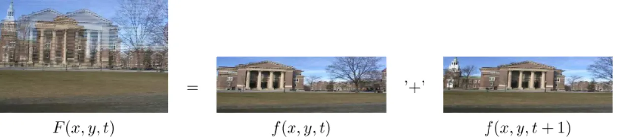
Most video cameras do not simultaneously record the even and odd scan lines of a single frame. In an interlaced video sequence, a field, f(x, y, t), at time t contains only one-half of the scan lines needed for a full-resolution frame, F(x, y, t). The second half of the scan lines, f(x, y, t+ 1), is recorded at time t+ 1. If the even and odd fields are simply woven together, as shown in the exaggerated example in Figure 2.1, the motion between times

t and t+ 1 leads to a “combing” artifact. The magnitude of this effect depends on the amount of motion between fields. In this section, we describe a technique for detecting tampering in interlaced video. We show that the motion between the fields of a single frame and across the fields of neighboring frames in an interlaced video should be equal. We propose an efficient way to measure these motions and show how tampering can disturb this relationship. Then, we show the efficacy of our approach on simulated and visually plausible forgeries.

2.1

Temporal Correlations in Interlaced Video

We begin by assuming that the motion is constant across at least three sequential fields. At a typical frame rate of 30 frames/second, this amounts to assuming that the motion is constant for 1/20 of a second (assuming that the time between fields is 1/60thof a second). Consider the fieldsf(x, y,1),f(x, y,2) andf(x, y,3) corresponding to the odd and even lines for frameF(x, y,1) and the odd lines for frame F(x, y,2), respectively. With the constant

(15)

= ’+’

F(x, y, t) f(x, y, t) f(x, y, t+ 1)

Figure 2.1: One half of the scan lines,f(x, y, t), of a full video frame are recorded at timet, and the other half of the scan lines,f(x, y, t+ 1) are recorded at timet+ 1. An interlaced frame,F(x, y, t), is created by simply weaving together these two fields.

motion assumption, we expect the inter-field motion between f(x, y,1) and f(x, y,2) to be the same as the inter-frame motion between f(x, y,2) and f(x, y,3). While the overall motion may change over time, this equality should be relatively constant. We will show below how to estimate this motion and how tampering can disturb this temporal pattern. For computational efficiency, we convert each RGB frame to grayscale (gray = 0.299R + 0.587G + 0.114B ) – all three color channels could be analyzed and their results averaged1.

2.1.1 Motion Estimation

We consider a classic differential framework for motion estimation [19, 1, 48]. We begin by assuming that the image intensities between fields are conserved (the brightness constancy assumption), and that the motion between fields can locally be modeled with a 2-parameter translation. The following expression embodies these two assumptions:

f(x, y, t) =f(x+vx, y+vy, t−1), (2.1)

where the motion is~v= vx vy

T

. In order to estimate the motion~v, we define the following quadratic error function to be minimized:

E(~v) = X x,y∈Ω f(x, y, t)−f(x+vx, y+vy, t−1) 2 , (2.2) 1

Since the color channels are correlated, we expect little advantage to averaging the motion estimated from each of the three color channels.

(16)

where Ω denotes a spatial neighborhood. Since this error function is non-linear in its un-knowns, it cannot be minimized analytically. To simplify the minimization, we approximate this error function using a first-order truncated Taylor series expansion:

E(~v)≈ X x,y∈Ω f(x, y, t)−(f(x, y, t) +vxfx(x, y, t) +vyfy(x, y, t)−ft(x, y, t)) 2 = X x,y∈Ω f −(f +vxfx+vyfy−ft) 2 , (2.3)

wherefx(·), fy(·), andft(·) are the spatial and temporal derivatives off(·), and where for notational convenience the spatial/temporal parameters are dropped. This error function reduces to: E(~v) = X x,y∈Ω ft−vxfx−vyfy 2 = X x,y∈Ω " ft− fx fy    vx vy    #2 = X x,y∈Ω ft−f~s T ~ v2. (2.4)

Note that this quadratic error function is now linear in its unknowns,~v. This error function can be minimized analytically by differentiating with respect to the unknowns:

dE(~v) d~v = X x,y∈Ω −2f~s ft−f~s T ~ v (2.5)

and setting this result equal to zero, and solving for~v:

~v=−    P Ωfx2 P Ωfxfy P Ωfxfy PΩfy2    −1   P Ωfxft P Ωfyft   , (2.6)

where again recall that the spatial/temporal parameters on the derivatives have been dropped for notational convenience. This solution assumes that the first term, a 2×2 matrix, is invertible. This can usually be guaranteed by integrating over a large enough spatial neighborhood Ω with sufficient image content.

(17)

2.1.2 Spatial/Temporal Differentiation

The spatial/temporal derivatives needed to estimate motion in Equation (2.6) are deter-mined via convolutions [11] as follows:

fx= (1₂ft(x, y, t) +1₂ft(x, y, t−1))? d(x)? p(y) (2.7)

fy = (1₂ft(x, y, t) +1₂ft(x, y, t−1))? p(x)? d(y) (2.8)

ft= (1₂ft(x, y, t)−1₂ft(x, y, t−1))? p(x)? p(y), (2.9)

where the 1-D filters ared(·) =0.425287 0.0 −0.425287andp(·) =0.2298791 0.540242 0.2298791. Note that while we employ 2-tap filters for the temporal filtering ( 1₂ 1₂ and

1 2 −

1 2

), 3-tap filters are used for the spatial filtering. Despite the asymmetry, these filters yield more accurate motion estimates. To avoid edge artifacts due to the convolution, the derivatives are centrally cropped by removing a 2-pixel border.

2.1.3 Inter-Field and Inter-Frame Motion

Recall that we are interested in comparing the inter-field motion between f(x, y, t) and

f(x, y, t + 1) and the inter-frame motion between f(x, y, t + 1) and f(x, y, t+ 2), for t

odd. The inter-field motion is estimated in a two-stage process (the inter-frame motion is computed in the same way).

In the first stage, the motion is estimated globally between f(x, y, t) and f(x, y, t+ 1), that is, Ω is the entire image in Equation (2.6). The second field,f(x, y, t+1), is then warped according to this estimated motion (a global translation). This stage removes any large-scale motion due to, for example, camera motion. In the second stage, the motion is estimated locally for non-overlapping blocks of size Ω =n×npixels. This local estimation allows us to consider more complex and spatially varying motions, other than global translation. For a given block, the overall motion is then simply the sum of the global and local motion.

The required spatial/temporal derivatives have finite support thus fundamentally limit-ing the amount of motion that can be estimated. By sub-sampllimit-ing the images, the motion is typically small enough for our differential motion estimation. In addition, the run-time

(18)

is sufficiently reduced by operating on sub-sampled images. In both stages, therefore, the motion estimation is done on a sub-sampled version of the original fields: a factor of 16 for the global stage, and a factor of 8 of the local stage, with Ω = 13×13 (correspond-ing to a neighborhood size of 104×104 at full resolution). While the global estimation, done at a coarser scale, yields a less accurate estimation of motion, it does remove any large-scale motion. The local stage done at a higher scale then refines this estimate. For computational considerations, we do not consider other scales, although this could easily be incorporated. To avoid wrap-around edge artifacts due to the global alignment correction, six pixels are cropped along each horizontal edge and two pixels along each vertical edge prior to estimating motion at 1/8 resolution.

In order to reduce the errors in motion estimation, the motion across three pairs of fields is averaged together, where the motion between each pair is computed as described above. The inter-frame motion is estimated in the same way, and the norm of the two motions,

k~vk=

q v2

x+v2y, are compared across the entire video sequence.

2.2

Results

An interlaced video sequence, F(x, y, t), of length T frames is first separated into fields,

f(x, y, t) with t odd corresponding to the odd scan lines and t even corresponding to the even scan lines. The inter-field motion is measured as described above for all pairs of fields

f(x, y, t) andf(x, y, t+ 1), for t odd, and the inter-frame motion is measured between all pairs of fields f(x, y, t+ 1) and f(x, y, t+ 2), for 3 ≤ t ≤ 2T −3. We expect these two motions to be the same in an authentic interlaced video, and to be disrupted by tampering. We recorded three videos from a SONY-HDR-HC3 digital video camera. The camera was set to record in interlaced mode at 30 frames/sec. Each frame is 480×720 pixels in size, and the average length of each video sequence is 10 minutes or 18,000 frames. For the first video sequence, the camera was placed on a tripod and pointed towards a road and sidewalk, as a surveillance camera might be positioned. For the two other sequences, the camera was hand-held.

(19)

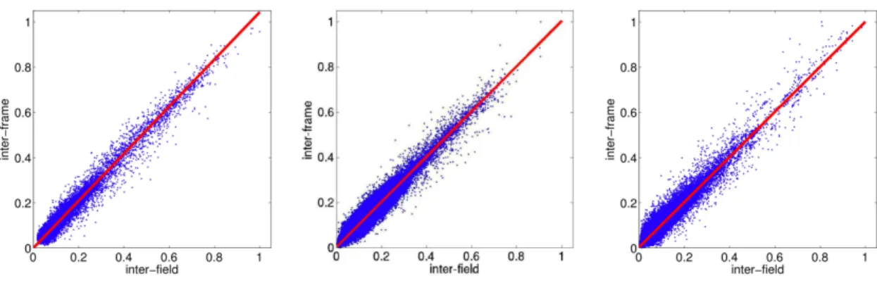
Figure 2.2: Shown in each panel is the normalized field motion versus the normalized inter-frame motion for three different video sequences. The solid line represents a line fit to the underlying data points. We expect the motion ratio to be near 1 in an authentic video sequence and to deviate significantly for a doctored video.

sequence. Each data point corresponds to the estimate from a single 13×13 block (at 1/8 resolution). Since we are only interested in the motion ratio, the motions are normalized into the range [0,1]. Also shown in each panel is a line fit to the underlying data (solid line), which in the ideal case would be a unit-slope line with zero intercept. The average motion ratio for each sequence is 0.98, 0.96, and 0.98 with a variance of 0.008, 0.128, and 0.156, respectively.

A frame is classified as manipulated if at least one block in the frame has a motion ratio that is more than 0.2 from unit value. In order to avoid spurious errors, we also insist that at least 3 successive frames are classified as manipulated. For the first video sequence, only one block out of 221,328 blocks was incorrectly classified as manipulated. For the second and third sequence, two and eight blocks, respectively, were misclassified out of a total of 241,248 and 224,568 blocks. After imposing the temporal constraints, no frames were mis-classified.

Shown in the first two rows of Figure 2.3 are ten frames of an original interlaced video. This video shows a person walking against a stationary background and being filmed with a stationary camera. Shown in the next two rows of this same figure is a doctored version of this video sequence. In this version, a different person’s head has been spliced into each frame. Because this person was walking at a slower speed than the original person, the inter-field interlacing is smaller than in the original. Shown in lower portion of Figure 2.3 are the resulting inter-field and inter-frame motions. The data points that lie significantly

(20)

away from the unit-slope line correspond to the blocks in which the new head was introduced – occasionally this would occupy two blocks, both of which would deviate from the expected motion ratio. Even though the doctored video looks perceptually smooth, the tampering is easily detected.

Since compression will introduce perturbations into the image, it is important to test the sensitivity of the motion estimation algorithms to compression. The first video sequence described above was compressed using Adobe Premiere to a target bit rate of 9, 6, and 3 Mbps. The same inter-field and inter-frame motions were estimated for each of these video sequences. For the original sequence, only 1 block out of 221,328 blocks was incorrectly classified as manipulated. After the temporal filtering, no frames out of 18,444 frames were incorrectly classified. For the three compressed video sequences, 1, 4, and 3 blocks were mis-classified, and 0, 1, and 0 frames were mis-classified. The motion estimation algorithm is largely insensitive to compression artifacts. One reason for this is that we operate on a sub-sampled version of the video (by a factor of 1/16 and 1/8) in which many of the compression artifacts are no longer present. In addition, the motion is estimated over a spatial neighborhood so that many of the errors are integrated out.

2.2.1 Frame Rate Down-Conversion

This technique can be adapted to detect frame rate down-conversion. Consider an original video sequence captured at 30-frames per second that is subsequently manipulated and saved at a lower rate of 25-frames per second. The standard approach to reducing the frame rate is to simply remove the necessary number of frames (5 per second in this example). In so doing, the inter-field and inter-frame motion ratio as described in the previous section will be disturbed. Specifically at the deleted frames, the inter-field motion will be too small relative to the inter-frame motion.

A video sequence of length 1200 frames, originally recorded at 30 frames per second, was converted using VirtualDub to a frame rate of 25 frames per second, yielding a video of length 1000 frames. The inter-field and inter-frames motions were estimated as described. In this frame rate converted video every 5th frame had an average motion ratio of 2.91, while the intervening frames had an average motion ratio of 1.07.

(21)

Figure 2.3: Shown in the top two rows are 10 frames of an original interlaced video. Shown in the next two rows is a doctored version of this video sequence, and in the lower-left are enlargements of the last frame of the original and doctored video. The plot shows the field versus the inter-frame motion – the data points that lie significantly away from the unit slope line correspond to doctored blocks (the head) while the data points on the line correspond to the original blocks (the body).

(22)

2.3

Discussion

We have presented a technique for detecting tampering in interlaced video. We measure the inter-field and inter-frame motions which for an authentic video are the same, but for a doctored video may be different. This technique can localize tampering both in time and space. It can also be adapted slightly to detect frame rate down-conversion. Compression artifacts have little effect on the estimation of motion in interlaced video, so this approach is appropriate for a range of interlaced video. The weakness of this method is that it cannot detect manipulations in regions where there is no motion, since in this case the inter-field and inter-frame motion are constantly zero.

Counterattacking this technique would be relatively difficult as it would require the forger to locally estimate the inter-frame motions and interlace the doctored video so as to match the inter-field and inter-frame motions.

(23)

Chapter 3

De-Interlaced

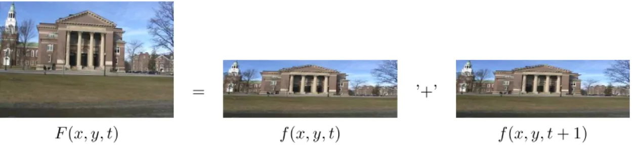
In Chapter 2, we described a technique to detect tampering in interlaced video. Inter-laced video usually has spatial “combing” artifacts for quickly moving objects. In order to minimize these artifacts, a de-interlaced video will combine the even and odd lines in a more sensible way (see Figure 3.1), usually relying on some form of spatial and tempo-ral interpolation (see [7] for a genetempo-ral overview and [8, 49, 2, 41] for specific and more advanced approaches). In this section, we describe a technique for detecting tampering in de-interlaced video. We quantify the correlations introduced by the camera or software de-interlacing algorithms and show how tampering can disturb these correlations. Then, we show the efficacy of our approach on simulated and visually plausible forgeries.

3.1

De-Interlacing Algorithms

There are two basic types of de-interlacing algorithms: field combination and field extension. Given an interlaced video of length T fields, a field combination de-interlacing algorithm yields a video of length T /2 frames, where neighboring fields in time are combined into a single frame. A field extension de-interlacing algorithm yields a video of length T, where each field in time is extended into one frame. We will constrain ourselves to field extension algorithms. For notational simplicity, we assume that the odd/even scan lines are inserted into frames F(x, y, t) with odd/even values of t, respectively. Below we describe several field extension de-interlacing algorithms, some of which are commonly found in commercial

(24)

= ’+’

F(x, y, t) f(x, y, t) f(x, y, t+ 1)

Figure 3.1: One half of the scan lines,f(x, y, t), of a full video frame are recorded at timet, and the other half of the scan lines, f(x, y, t+ 1), are recorded at time t+ 1. A de-interlaced frame,

F(x, y, t), is created by combining these two fields to create a full frame.

video cameras.

3.1.1 Line Repetition

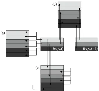
In this simplest of de-interlacing algorithms, Figure 3.2(a), the scan lines of each field,

f(x, y, t), are duplicated to create a full frame,F(x, y, t):

F(x, y, t) =f(x,dy/2e, t). (3.1)

While easy to implement, the final de-interlaced video suffers from having only one-half the vertical resolution as compared to the horizontal resolution.

3.1.2 Field Insertion

In this de-interlacing algorithm, Figure 3.2(b), neighboring fields, f(x, y, t), are simply combined to create a full frame,F(x, y, t). For odd values oft:

F(x, y, t) =      f(x,(y+ 1)/2, t) ymod 2 = 1 f(x, y/2, t+ 1) ymod 2 = 0 , (3.2)

and for even values of t:

F(x, y, t) =      f(x, y/2, t) ymod 2 = 0 f(x,(y+ 1)/2, t+ 1) ymod 2 = 1 . (3.3)

(25)

That is, for odd values of t, the odd scan lines of the full frame are composed of the field at timet, and the even scan lines of the full frame are composed of the field at time t+ 1. Similarly, for even values oft, the even scan lines of the full frame are composed of the field at timet, and the odd scan lines of the full frame are composed of the field at time t+ 1.

Unlike the line repetition algorithm, the final de-interlaced video has the full vertical resolution. Significant motion between the fields, however, introduces artifacts into the final video due to the mis-alignment of the fields. This artifact manifests itself with the commonly seen “combing effect”.

3.1.3 Line Averaging

In this easy to implement and popular technique, Figure 3.2(c), neighboring scan lines,

f(x, y, t), are averaged together to create the necessary scan lines of the full frame,F(x, y, t). For odd values oft:

F(x, y, t) =      f(x,(y+ 1)/2, t) ymod 2 = 1 1 2f(x, y/2, t) + 1 2f(x, y/2 + 1, t) ymod 2 = 0 , (3.4)

and for even values of t:

F(x, y, t) =      f(x, y/2, t) ymod 2 = 0 1 2f(x,(y+ 1)/2−1, t) + 1 2f(x,(y+ 1)/2, t) ymod 2 = 1 . (3.5)

Where necessary, boundary conditions (the first and last scan lines) can be handled by employing line repetition. This algorithm improves on the low vertical resolution of the line repetition algorithm, while avoiding the combing artifacts of the field insertion algorithm.

3.1.4 Vertical Temporal Interpolation

Similar to the line averaging algorithm, the vertical temporal interpolation algorithm com-bines neighboring scan lines in space (and here, in time), f(x, y, t) and f(x, y, t+ 1), to

(26)

create the necessary scan lines of the full frame, F(x, y, t). For odd values oft: F(x, y, t) =                    f(x,(y+ 1)/2, t) ymod 2 = 1 c1f(x, y/2−1, t) +c2f(x, y/2, t) +c3f(x, y/2 + 1, t)+ c4f(x, y/2 + 2, t) +c5f(x, y/2−1, t+ 1)+ c6f(x, y/2, t+ 1) +c7f(x, y/2 + 1, t+ 1) ymod 2 = 0 . (3.6) While the specific numeric weights ci may vary, a typical example is c1 = 1/18, c2 = 8/18, c3= 8/18,c4= 1/18,c5 =−5/18, c6= 10/18, andc7 =−5/18. For even values of t:

F(x, y, t) =                            f(x, y/2, t) ymod 2 = 0 c1f(x,(y+ 1)/2−2, t) +c2f(x,(y+ 1)/2−1, t)+ c3f(x,(y+ 1)/2, t) +c4f(x,(y+ 1)/2 + 1, t)+ c5f(x,(y+ 1)/2−1, t+ 1) +c6f(x,(y+ 1)/2, t+ 1)+ c7f(x,(y+ 1)/2 + 1, t+ 1) ymod 2 = 1 . (3.7) Where necessary, boundary conditions can be handled by employing line repetition. As with the line averaging algorithm, this algorithm improves the vertical temporal resolution. By averaging over a larger spatial and temporal neighborhood, the resolution can be improved beyond line averaging. By incorporating temporal neighborhoods, however, this algorithm is vulnerable to the combing artifacts of the field insertion algorithm.

3.1.5 Motion Adaptive

There is a natural tradeoff between de-interlacing algorithms that create a frame from only a single field (e.g., line repetition and line averaging) and those that incorporate two or more fields (e.g., field insertion and vertical temporal interpolation). In the former case, the resulting de-interlaced video suffers from low vertical resolution but contains no combing artifacts due to motion between fields. In the latter case, the de-interlaced video has an optimal vertical resolution when there is no motion between fields, but suffers from combing artifacts when there is motion between fields.

(27)

Figure 3.2: Illustrated in this schematic are the (a) line repetition, (b) field insertion and (c) line averaging de-interlacing algorithms. The individual fields,f(x, y, t) andf(x, y, t+ 1), are illustrated with three scan lines each, and the full de-interlaced frames are illustrated with six scan lines.

Motion adaptive algorithms incorporate the best of these techniques to improve vertical resolution while minimizing combing artifacts. While specific implementations vary, the basic algorithm creates two de-interlaced sequences, F1(x, y, t) and F2(x, y, t), using, for example, field insertion and line repetition. Standard motion estimation algorithms are used to create a “motion map”, α(x, y) with values of 1 corresponding to regions with motion and values of 0 for regions with no motion. The final de-interlaced video is then given by:

F(x, y, t) = (1−α(x, y))F1(x, y, t) +α(x, y)F2(x, y, t). (3.8)

Although more complicated to implement due to the need for motion estimation, this algo-rithm affords good vertical resolution with minimal motion artifacts.

3.1.6 Motion Compensated

In this approach, standard motion estimation algorithms are employed to estimate the motion between neighboring fields,f(x, y, t) andf(x, y, t+ 1). The resulting motion field is used to warp f(x, y, t+ 1) in order to undo any motion that occurred between fields. The resulting new field, f0(x, y, t+ 1) is then combined with the first field,f(x, y, t) using field

(28)

insertion, Section 3.1.2. The benefit of this approach is that the resulting de-interlaced video is of optimal vertical resolution with no motion artifacts (assuming good motion estimation). The drawback is that of added complexity due to the need for motion estimation and possible artifacts due to poor motion estimates.

3.2

Spatial/Temporal Correlations in De-Interlaced Video

Given a de-interlaced video generated with any of the above algorithms, we seek to model the spatial and temporal correlations that result from the de-interlacing. The approach we take is similar in spirit to [45], where we modeled color filter array interpolation algorithms. Consider, for example, the line averaging algorithm in which every other scan line is linearly correlated to its neighboring scan line, Equation (3.4). In this case:

F(x, y, t) = 1₂F(x, y−1, t) +1₂F(x, y+ 1, t) (3.9)

for either odd or even values of y. The remaining scan lines do not necessarily satisfy this relationship.

Consider for now, only the odd scan lines, Fo(x, y, t), ofF(x, y, t) forteven (the formu-lation for Fe(x, y, t) is identical). If this frame has not been doctored, then we expect that every pixel of Fo(x, y, t) will be correlated to its spatial and temporal neighbors. Regions that violate this relationship indicate tampering. As such, we seek to simultaneously seg-ment Fo(x, y, t) into those pixels that are linearly correlated to their spatial and temporal neighbors and those that are not, and to estimate these correlations. We choose a linear model since it is a good model for most de-interlacing algorithms.

The expectation/maximization (EM) algorithm is employed to solve this simultaneous segmentation and estimation problem. We begin by assuming that each pixel ofFo(x, y, t) belongs to one of two models, M1 orM2. Those pixels that belong to M1 satisfy:

Fo(x, y, t) = X i∈{−3,−1,1,3} αiF(x, y+i, t) + X i∈{−2,0,2} βiF(x, y+i, t+ 1) + n(x, y), (3.10)

(29)

belong to M2 are considered to be generated by an “outlier” process. Note that Equa-tion (3.10) embodies all of the de-interlacing algorithms described in the previous secEqua-tions, except for the motion compensated algorithm (more on this later).

The EM algorithm is a two-step iterative algorithm: (1) in the E-step the probability of each pixel belonging to each model is estimated; and (2) in the M-step the specific form of the correlations between pixels is estimated. More specifically, in the E-step, the probability of each pixel of Fo(x, y, t) belonging to modelM1 is estimated using Bayes’ rule:

P{Fo(x, y, t)∈M1|Fo(x, y, t)}= P{Fo(x, y, t) |Fo(x, y, t)∈M1}P{Fo(x, y, t)∈M1} P2 i=1P{Fo(x, y, t) |Fo(x, y, t)∈Mi}P{Fo(x, y, t)∈Mi} , (3.11) where the prior probabilities P{Fo(x, y, t) ∈ M1} and P{Fo(x, y, t) ∈ M2} are each as-sumed to be equal to 1/2. The probability of observing a sampleFo(x, y, t) knowing it was generated from model M1 is given by:

P{Fo(x, y, t) |Fo(x, y, t)∈M1}= 1 σ√2πexp   − Fo(x, y, t)−F˜o(x, y, t) 2 2σ2   , (3.12) where: ˜ Fo(x, y, t) = X i∈{−3,−1,1,3} αiF(x, y+i, t) + X i∈{−2,0,2} βiF(x, y+i, t+ 1). (3.13)

The variance, σ2, of this Gaussian distribution is estimated in the M-step. A uniform distribution is assumed for the probability of observing a sample generated by the outlier model, M2, i.e., P{Fo(x, y, t) |Fo(x, y, t)∈M2} is equal to the inverse of the range of possible values of Fo(x, y, t).

Note that the E-step requires an estimate of the coefficients αi and βi, which on the first iteration is chosen randomly. In the M-step, a new estimate of these model parame-ters is computed using weighted least squares, by minimizing the following quadratic error function: E({αi, βi}) = X x,y w(x, y) Fo(x, y, t)−F˜o(x, y, t) 2 , (3.14)

(30)

where the weights w(x, y) ≡ P{Fo(x, y, t) ∈M1 | Fo(x, y, t)}, Equation (3.11). This error function is minimized by computing the partial derivative with respect to each αi and βi, setting each of the results equal to zero and solving the resulting system of linear equations. The derivative, for example, with respect toαj is:

X x,y w(x, y)F(x, y+j, t)Fo(x, y, t) = X i∈{−3,−1,1,3} αi X x,y w(x, y)F(x, y+i, t)F(x, y+j, t) ! + X i∈{−2,0,2} βi X x,y w(x, y)F(x, y+i, t+ 1)F(x, y+j, t) ! . (3.15)

The derivative with respect toβj is:

X x,y w(x, y)F(x, y+j, t+ 1)Fo(x, y, t) = X i∈{−3,−1,1,3} αi X x,y w(x, y)F(x, y+i, t)F(x, y+j, t+ 1) ! + X i∈{−2,0,2} βi X x,y w(x, y)F(x, y+i, t+ 1)F(x, y+j, t+ 1) ! . (3.16)

Computing all such partial derivatives yields a system of seven linear equations in the seven unknowns αi and βi. This system can be solved using standard least-squares estimation. The variance,σ2_{, for the Gaussian distribution is also estimated on each M-step, as follows:}

σ2= P x,yw(x, y)(Fo(x, y, t)−F˜o(x, y, t))2 P x,yw(x, y) . (3.17)

The E-step and M-step are iteratively executed until stable estimates of αi and βi are obtained.

3.3

Results

Shown in the top portion of Figure 3.3 are eleven frames from a 250-frame long video sequence. Each frame is of size 480×720 pixels. Shown in the bottom portion of this figure

(31)

are the same eleven frames de-interlaced with the line average algorithm. This video was captured with a Canon Elura digital video camera set to record in interlaced mode. The interlaced video was de-interlaced with our implementation of line repetition, field insertion, line average, vertical temporal integration, motion adaptive, and motion compensated, and the de-interlacing plug-in for VirtualDub 1 which employs the motion adaptive algorithm.

In each case, each frame of the video was analyzed using the EM algorithm. The EM algorithm returns both a probability map denoting which pixels are correlated to their spatial/temporal neighbors, and the coefficients of this correlation. For simplicity, we report on the results for only the odd frames (in all cases, the results for the even frames are comparable). Within an odd frame, only the even scan lines are analyzed (similarly for the odd scan lines on the even frames). In addition, we convert each frame from RGB to grayscale (gray = 0.299R + 0.587G + 0.114B) – all three color channels could easily be analyzed and their results combined via a simple voting scheme.

Shown below is the percentage of pixels classified as belonging to modelM1, that is, as being correlated to their spatial neighbor:

de-interlace accuracy

line repetition 100% field insertion 100% line average 100% vertical temporal 99.5%

motion adaptive (no-motion|motion) 97.8% |100% motion compensation 97.8%

VirtualDub (no-motion|motion) 99.9% |100%

A pixel is classified as belonging to M1 if the probability, Equation (3.11), is greater than 0.90. The small fraction of pixels that are incorrectly classified are scattered across frames, and can thus easily be seen to not be regions of tampering – a spatial median filter would easily remove these pixels, while not interfering with the detection of tampered regions (see below). For de-interlacing by motion adaptive and VirtualDub, the EM algorithm was run separately on regions of the image with and without motion. Regions of motion

1

(32)

Figure 3.3: Shown in the top portion are eleven frames of a 250-frame long video sequence. Shown in the bottom portion are the same eleven frames de-interlaced using the line average algorithm – notice that the interlacing artifacts are largely reduced. Shown in the lower-right corner is an enlargement of the pedestrian’s foot from the last frame.

(33)

are determined simply by computing frame differences – pixels with an intensity difference greater than 3 (on a scale of [0,255] are classified as having undergone motion, with the remaining pixels classified as having no motion. The reason for this distinction is that the motion adaptive algorithm, Section 3.1.5, employs different de-interlacing for regions with and without motion. Note that for de-interlacing by motion compensation, only pixels with no motion are analyzed. The reason is that in this interlacing algorithm, the de-interlacing of regions with motion does not fit our model, Equation (3.10).

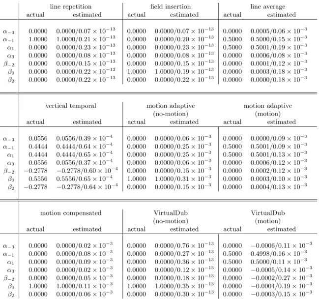
Shown in Figure 3.4 are the actual and estimated (mean/standard deviation) model coefficients,αi and βi, averaged over the entire video sequence. Note that, in all cases, the mean estimates are very accurate. The standard deviations range from nearly zero (10−13) to relatively small (10−4−10−3). The reason for these differences is two-fold: (1) rounding errors are introduced for the de-interlacing algorithms with non-integer coefficientsαi and

βi, and (2) errors in the motion estimation for the motion-adaptive based algorithms which incorrectly classifies pixels as having motion or no-motion.

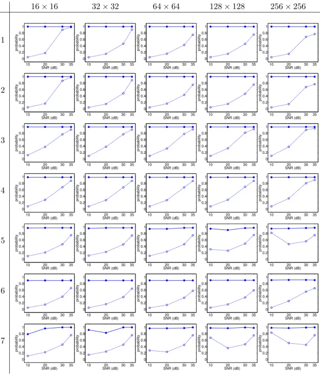
Shown in Figure 3.5 are results for detecting tampering in the video sequence of Fig-ure 3.3. We simulated the effects of tampering by adding, into a central square region of varying size, white noise of varying signal to noise ratio (SNR). A unique noise pattern was added to each video frame. The motivation behind this manipulation is that, as would most forms of tampering, the noise destroys the underlying de-interlacing correlations. The tampered regions were of size 256×256, 128×128, 64×64, 32×32 or 16×16 pixels, in each frame of size 480×720. The SNR, 10, 20, 30 or 35 dB, ranges from the highly visible (10 dB) to perceptually invisible (35 dB). Shown in each panel of Figure 3.5 is the average probability, over all frames, as reported by the EM algorithm for the central tampered re-gion and the surrounding untampered rere-gion. This probability corresponds to the likelihood that each pixel is correlated to their spatial and temporal neighbors (i.e., is consistent with the output of a de-interlacing algorithm). We expect probabilities significantly less than 1 for the tampered regions, and values close to 1 for the untampered region. For the motion adaptive algorithms, we combined the probabilities for the motion and no-motion pixels.

Notice that in general, detection is quite easy for SNR values below 25dB, that is, the tampered region has an average probability significantly less than the untampered region.

(34)

line repetition field insertion line average actual estimated actual estimated actual estimated

α−3 0.0000 0.0000/0.07×10−13 0.0000 0.0000/0.07×10−13 0.0000 0.0005/0.06×10−3 α−1 1.0000 1.0000/0.21×10−13 0.0000 0.0000/0.20×10−13 0.5000 0.5000/0.15×10−3 α1 0.0000 0.0000/0.23×10−13 0.0000 0.0000/0.23×10−13 0.5000 0.5001/0.19×10−3 α3 0.0000 0.0000/0.08×10−13 0.0000 0.0000/0.08×10−13 0.0000 0.0006/0.08×10−3 β−2 0.0000 0.0000/0.15×10−13 0.0000 0.0000/0.15×10−13 0.0000 0.0001/0.12×10−3 β0 0.0000 0.0000/0.22×10−13 1.0000 1.0000/0.19×10−13 0.0000 0.0003/0.18×10−3 β2 0.0000 0.0000/0.22×10−13 0.0000 0.0000/0.22×10−13 0.0000 0.0000/0.18×10−3

vertical temporal motion adaptive motion adaptive (no-motion) (motion) actual estimated actual estimated actual estimated

α−3 0.0556 0.0556/0.39×10−4 0.0000 0.0000/0.06×10−3 0.0000 0.0000/0.09×10−3 α−1 0.4444 0.4444/0.64×10−4 0.0000 0.0000/0.25×10−3 0.5000 0.5001/0.09×10−3 α1 0.4444 0.4444/0.65×10−4 0.0000 0.0000/0.25×10−3 0.5000 0.5001/0.13×10−3 α3 0.0556 0.0556/0.37×10−4 0.0000 0.0000/0.06×10−3 0.0000 0.0006/0.12×10−3 β−2 −0.2778 −0.2778/0.60×10−4 0.0000 0.0000/0.15×10−3 0.0000 0.0002/0.12×10−3 β0 0.5556 0.5556/0.65×10−4 1.0000 1.0000/0.31×10−3 0.0000 0.0003/0.10×10−3 β2 −0.2778 −0.2778/0.64×10−4 0.0000 0.0000/0.15×10−3 0.0000 0.0004/0.13×10−3

motion compensated VirtualDub VirtualDub (no-motion) (motion) actual estimated actual estimated actual estimated

α−3 0.0000 0.0000/0.02×10−3 0.0000 0.0000/0.76×10−13 0.0000 −0.0006/0.11×10−3 α−1 0.0000 0.0000/0.08×10−3 0.0000 0.0000/0.27×10−13 0.5000 0.4998/0.16×10−3 α1 0.0000 0.0000/0.09×10−3 0.0000 0.0000/0.36×10−13 0.5000 0.5000/0.11×10−3 α3 0.0000 0.0000/0.02×10−3 0.0000 0.0000/0.12×10−13 0.0000 −0.0005/0.14×10−3 β−2 0.0000 0.0000/0.05×10−3 0.0000 0.0000/0.18×10−13 0.0000 −0.0002/0.27×10−3 β0 1.0000 1.0000/0.11×10−3 1.0000 1.0000/0.35×10−13 0.0000 −0.0004/0.19×10−3 β2 0.0000 0.0000/0.06×10−3 0.0000 0.0000/0.30×10−13 0.0000 −0.0003/0.15×10−3

Figure 3.4: Shown are the actual and estimated (mean/standard deviation) model coefficients for the video sequence of Figure 3.3 that was de-interlaced with the specified algorithms.

Notice also that the detection gets slightly easier for larger regions, particularly at high SNR values, but that even very small regions (16×16) are still detectable. And finally, note that in the case of de-interlacing by motion adaptive and VirtualDub, the tampered regions are more difficult to detect for large regions with low SNR (rows 5 and 7, last column). The reason for this is the large tampered regions at a low SNR give rise to a significant number of pixels mistakenly classified as having motion or no motion. As a result, the value ofσ in Equation (3.12) increases, which naturally results in a larger probability for the tampered region. Note however, that the final probability is still below the 0.90 threshold used to

(35)

16×16 32×32 64×64 128×128 256×256 1 10 20 30 35 0 0.2 0.4 0.6 0.8 1 SNR (dB) probability 10 20 30 35 0 0.2 0.4 0.6 0.8 1 SNR (dB) probability 10 20 30 35 0 0.2 0.4 0.6 0.8 1 SNR (dB) probability 10 20 30 35 0 0.2 0.4 0.6 0.8 1 SNR (dB) probability 10 20 30 35 0 0.2 0.4 0.6 0.8 1 SNR (dB) probability 2 10 20 30 35 0 0.2 0.4 0.6 0.8 1 SNR (dB) probability 10 20 30 35 0 0.2 0.4 0.6 0.8 1 SNR (dB) probability 10 20 30 35 0 0.2 0.4 0.6 0.8 1 SNR (dB) probability 10 20 30 35 0 0.2 0.4 0.6 0.8 1 SNR (dB) probability 10 20 30 35 0 0.2 0.4 0.6 0.8 1 SNR (dB) probability 3 10 20 30 35 0 0.2 0.4 0.6 0.8 1 SNR (dB) probability 10 20 30 35 0 0.2 0.4 0.6 0.8 1 SNR (dB) probability 10 20 30 35 0 0.2 0.4 0.6 0.8 1 SNR (dB) probability 10 20 30 35 0 0.2 0.4 0.6 0.8 1 SNR (dB) probability 10 20 30 35 0 0.2 0.4 0.6 0.8 1 SNR (dB) probability 4 10 20 30 35 0 0.2 0.4 0.6 0.8 1 SNR (dB) probability 10 20 30 35 0 0.2 0.4 0.6 0.8 1 SNR (dB) probability 10 20 30 35 0 0.2 0.4 0.6 0.8 1 SNR (dB) probability 10 20 30 35 0 0.2 0.4 0.6 0.8 1 SNR (dB) probability 10 20 30 35 0 0.2 0.4 0.6 0.8 1 SNR (dB) probability 5 10 20 30 35 0 0.2 0.4 0.6 0.8 1 SNR (dB) probability 10 20 30 35 0 0.2 0.4 0.6 0.8 1 SNR (dB) probability 10 20 30 35 0 0.2 0.4 0.6 0.8 1 SNR (dB) probability 10 20 30 35 0 0.2 0.4 0.6 0.8 1 SNR (dB) probability 10 20 30 35 0 0.2 0.4 0.6 0.8 1 SNR (dB) probability 6 10 20 30 35 0 0.2 0.4 0.6 0.8 1 SNR (dB) probability 10 20 30 35 0 0.2 0.4 0.6 0.8 1 SNR (dB) probability 10 20 30 35 0 0.2 0.4 0.6 0.8 1 SNR (dB) probability 10 20 30 35 0 0.2 0.4 0.6 0.8 1 SNR (dB) probability 10 20 30 35 0 0.2 0.4 0.6 0.8 1 SNR (dB) probability 7 10 20 30 35 0 0.2 0.4 0.6 0.8 1 SNR (dB) probability 10 20 30 35 0 0.2 0.4 0.6 0.8 1 SNR (dB) probability 10 20 30 35 0 0.2 0.4 0.6 0.8 1 SNR (dB) probability 10 20 30 35 0 0.2 0.4 0.6 0.8 1 SNR (dB) probability 10 20 30 35 0 0.2 0.4 0.6 0.8 1 SNR (dB) probability

Figure 3.5: Shown in each panel is the probability that regions are consistent with de-interlacing as a function of signal to noise ratio (SNR) – the dashed line/open circle corresponds to tampered regions and the solid line/filled circle corresponds to untampered regions. Each column corresponds to a different tampered region size (in pixels), and each row corresponds to a different de-interlacing algorithm: (1) line repetition, (2) field insertion, (3) line average, (4) vertical temporal, (5) motion adaptive, (6) motion compensated, and (7) VirtualDub.

(36)

Figure 3.6: Four frames of a Britney Spears concert that have been doctored to include a dancing Marge and Homer Simpson. Shown below are the de-interlacing results that reveal the tampered region.

determine if a region has been tampered with.

Shown in Figure 3.6 are four frames of a doctored video sequence. The original video was de-interlaced with the vertical temporal algorithm. Each frame of the digitally inserted cartoon sequence was re-sized from its original destroying any de-interlacing correlations. Shown below each frame is the resulting probability map returned by the EM algorithm. The doctored region is clearly visible in each frame.

We naturally expect that various compression algorithms such as MPEG will somewhat disrupt the underlying correlations introduced by de-interlacing algorithms. To test the sen-sitivity to compression the 250-frame long video sequence described above was de-interlaced with the line repetition and line average algorithms, and then compressed using Adobe

(37)

Pre-miere to a target bit rate of 9, 6, and 3 Mbps. Below are the percentage of pixels classified as being correlated to their spatial neighbors.

de-interlace accuracy

none 9 Mbps 6 Mbps 3 Mbps line repetition 100% 97.1% 96.2% 93.2%

line average 100% 97.0% 96.0% 93.5%

Note that even when compressed, the de-interlacing artifacts can still be detected and that the accuracy degrades gracefully with increasing compression.

3.3.1 Frame Rate Up-Conversion

This technique can be adapted to detect frame rate up-conversion. Consider now a video sequence captured at 25-frames per second that is subsequently manipulated and saved at a higher rate of 30-frames per second. This frame rate conversion requires some form of interpolation in order to fill in the extra frames. There are several frame rate conversion algorithms that accomplish this. Frame repetition is the simplest approach where frames from the original sequence are simply repeated to expand the frame rate to the desired rate. When converting from 25 to 30 frames per second, for example, every fifth frame of the original sequence is duplicated. Linear frame rate conversion creates the extra frames by taking linear combinations of neighboring frames in time. More sophisticated motion-based algorithms compensate for the inter-frame motion in a similar way to the motion-based de-interlacing algorithms (e.g., [30, 3]).

Here we consider only the frame repetition and linear conversion techniques. The method we will describe can be adapted, as in the previous section, to be applicable to motion-based algorithms. For both algorithms, some frames in a converted video will be a linear combi-nation of their neighboring frames, while other frames will not. We therefore employ the EM algorithm to simultaneously segment the video into frames that are and are not linear combinations of their neighbors, and determine the linear coefficients of this combination.

(38)

Similar to before, the relationship between frames is modeled as:

F(x, y, t) = X i∈{−1,1}

αiF(x, y, t+i), (3.18)

where for simplicity only two temporal neighbors are considered – this could easily be expanded to consider a larger neighborhood. With a few minor changes, the EM algorithm described in the previous section can be adapted to detect frame rate conversion. Note first that the model here operates on entire frames, instead of individual pixels. Second, because the majority of frames will not correlated to their neighbors, we find that it is necessary to use a fixed, and relatively small, σ in Equation (3.12). And lastly, note that the model coefficients for the first frame in a duplicated pair will be α−1 = 0 and α1 = 1 while the coefficients for the second duplicated frame will beα−1 = 1 and α1 = 0. For our purposes, we would like to consider these models as the same. As such, on each EM iteration both the current and the symmetric version of the model coefficients are considered. The model that minimizes the residual error between the frame and the model is adopted.

A video sequence of length 960 frames, originally recorded at 25 frames per second, was converted using VirtualDub to a frame rate of 30 frames per second, yielding a video of length 1200 frames. VirtualDub employs a frame duplication algorithm. The EM algorithm detected that every multiple of 6 frames was a linear combination of their neighboring frames (with an average probability of 0.99), while the remaining frames were not (with an average probability of 0.00).

3.4

Discussion

We have presented a technique for detecting tampering in de-interlaced video. We explicitly model the correlations introduced by de-interlacing algorithms, and show how tampering can destroy these correlations. This technique can localize tampering both in time and in space and can also be slightly adapted to detect frame rate up-conversion that might result from video manipulation. Compression artifacts make it somewhat more difficult to estimate the de-interlacing correlations, so this approach is most appropriate for relatively

(39)

high quality video.

The model parameters for the untampered region of each frame are consistent through-out the entire sequence. Therefore, we can estimate one set of model parameters for all the frames together instead of for each frame separately. Due to the large amount of data in a video sequence, we need to reduce the computational complexity to a manageable scale. To do this, we can randomly sample pixels from the whole video sequence to provide the input data for the EM algorithm. Then the estimated model parameters are used to calculate the probability map for each frame. This approach can greatly reduce the computational cost because the EM algorithm is only applied once. At the same time, it also improves the accuracy of the estimation of the model parameters because the input data are no longer restricted to one frame.

One way to counterattack the de-interlacing forensic tool would be to recreate the cor-relations that were destroyed by the tampering. This could be achieved by first doctoring a video, then generating an interlaced video (split the even and odd scan lines), and finally applying a de-interlacing algorithm to generate a new de-interlaced video with intact corre-lations. If the original video camera is available, this approach requires the forger to employ the same de-interlacing algorithm as that used by the original camera.

(40)

Chapter 4

Double MPEG

MPEG is a well established video compression standard. In this chapter, we consider detecting tampering in videos compressed by MPEG. When an MPEG video is modified, and re-saved in MPEG format, it is subject to double compression. In this process, two types of artifacts – spatial and/or temporal – will likely be introduced into the resulting video. We describe how these artifacts can be quantified and estimated in order to detect forgeries. We begin by briefly describing the relevant components of MPEG video compression. Then we propose two techniques, each capable of capturing one type of double compression artifact, and show their efficacy in detecting tampering.

4.1

Video Compression

The MPEG video standard (MPEG-1 and MPEG-2) compresses video data by reduc-ing both spatial redundancy within individual frames and temporal redundancy across frames [47]. In this section, we give a brief overview of the MPEG standard.

4.1.1 Coding Sequence

In a MPEG encoded video sequence, there are three types of frames: intra (I), predictive (P) and bi-directionally predictive (B), each offering varying degrees of compression. These frames typically occur in a periodic sequence. A common sequence, for example, is:

(41)

where the subscripts are used to denote time. Such an encoding sequence is parameterized by the number of frames in a sequence, N, and the spacing of the P-frames, M. In the above sequence N = 12 and M = 3. Each N frames is referred to as a group of pictures (GOP).

I-frames are encoded without reference to any other frames in the sequence. P-frames are encoded with respect to the previous I- or P-frame, and offer increased compression overI-frames. B-frames are encoded with respect to the previous and next I- or P-frames and offer the highest degree of compression. In the next three sections,, these encodings are described in more detail.

4.1.2 I-frame

I-frames are typically the highest quality frames of a video sequence but afford the least amount of compression. I-frames are encoded using a fairly standard JPEG compression scheme. A color frame (RGB) is first converted into luminance/chrominance space (YUV). The two chrominance channels (UV) are subsampled relative to the luminance channel (Y), typically by a factor of 4 : 1 : 1. Each channel is then partitioned into 8×8 pixel blocks. A macroblock is then created by grouping together four such Y-blocks, one U-block, and one V-block in a 16×16 pixel neighborhood. After applying a discrete cosine transform (DCT) to each block, the resulting coefficients are quantized and run-length and variable-length encoded. The amount of quantization of the DCT coefficients depends on their spatial frequencies (higher frequencies are typically quantized more than lower frequencies). The DC coefficient (the (0,0) frequency) and the AC coefficients (all other frequencies) are quantized differently. Of our interest is the quantization of the AC coefficients, which is determined by two factors: the quantization table and the quantization scale. The quantization table specifies the quantization for each of 64 DCT frequencies in each YUV channel, and is generally held fixed across the entire video. The quantization scale (a scalar) can vary from frame to frame and from macroblock to macroblock, thus allowing the quantization to adapt to the local image structure. The final quantization for each DCT coefficient is then simply the product of the quantization table and scale.

(42)

4.1.3 P-frame

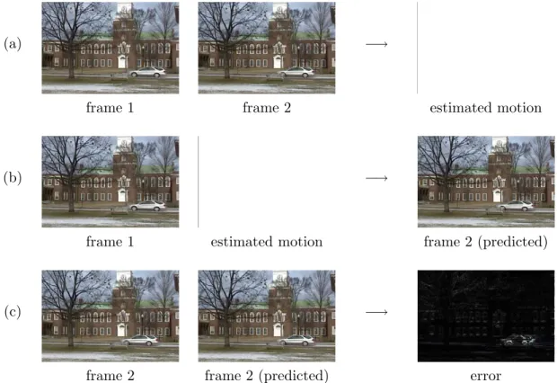
In the encoding of anI-frame, compression is achieved by reducing the spatial redundancies within a single video frame. The encoding of aP-frame is intended to reduce the temporal redundancies across frames, thus affording better compression rates. Consider for example a video sequence in which the motion between frames can be described by a single global translation. In this case, considerable compression can be achieved by encoding the first frame in the sequence and the amount of inter-frame motion (a single vector) for each subsequent frame. The original sequence can then be reconstructed by motion correcting (e.g., warping) the first frame according to the motion vectors. In practice, of course, a single motion vector is not sufficient to accurately capture the motion in most natural video sequences. As such, the motion between a P-frame and its preceding I- or P-frame is estimated for each 16×16 pixel block in the frame. A standard block-matching algorithm is typically employed for motion estimation, Figure 4.1(a). A motion estimated version of frame 2 can then be generated by warping the first frame according to the estimated motion, Figure 4.1(b). The error between this predicted frame, and the actual frame is then computed, Figure 4.1(c). Both the motion vectors and the motion errors are encoded and transmitted (the motion errors are statically encoded using a similar JPEG compression scheme as used for encoding I-frames). With relatively small motion errors, this scheme yields good compression rates. The decoding of a P-frame is then a simple matter of warping the previous frame according to the motion vector and adding the motion errors. By removing temporal redundancies, the P-frames afford better compression than the I -frames, but at a cost of a loss in quality. These frames are of lower quality because of the errors in motion estimation and the subsequent compression of the motion errors.

4.1.4 B-frame

Similar to aP-frame, aB-frame is encoded using motion compensation. Unlike aP-frame, however, a B-frame employs a past, future, or both of its neighboring I- or P-frames for motion estimation. By considering two moments in time, more accurate motion estimation is possible, and in turn better compression rates. The decoding of a B-frame requires that

(43)

(a) −→

frame 1 frame 2 estimated motion

(b) −→

frame 1 estimated motion frame 2 (predicted)

(c) −→

frame 2 frame 2 (predicted) error

Figure 4.1: Motion estimation is used to encodeP- andB-frames of a MPEG video sequence: (a) motion is estimated between a pair of video frames; (b) the first frame is motion compensated to produce a predicted second frame; and (c) the error between the predicted and actual second frame is computed. The motion estimation and errors are encoded as part of a MPEG video sequence.

both frames, upon which motion estimation relied, be transmitted first.

4.2

Spatial

We introduce a technique for detecting if a video frame or part of it was MPEG compressed twice as anI-frame. This manipulation might result from something as simple as recording an MPEG video, editing it, and re-saving it as another MPEG video. This manipulation might also arise from a more sophisticated green-screening in which two videos are compos-ited together. We show that such double compression introduces specific artifacts in the DCT coefficients of theI-frames of an MPEG video. In [43], Popescu et al. have described such double compression artifacts (see also [34]). In [51], we showed that such artifacts can be measured to detect doubly compressedI-frames. However, unlike these earlier tools, this technique can detect localized tampering in regions as small as 16×16 pixels.

(44)

4.2.1 Methods

The final quality of an MPEG video is determined by several factors. Among these is the amount of quantization applied to eachI-frame. Therefore, when anI-frame is compressed twice with different compression qualities, the DCT coefficients are subjected to two levels of quantization. Recall the final quantization is determined by two factors: the quantization table and the quantization scale. Since video encoders typically employ the default quanti-zation matrix, we assume that the variation in quantiquanti-zation is governed by the quantiquanti-zation scale.

Double Quantization

Consider a DCT coefficientu. In the first compression, the quantized DCT coefficientx is given by: x = u q1 , (4.1)

where q1 (a strictly positive integer) is the first quantization step, and [·] is the rounding function. When the compressed video is decoded to prepare for the second compression, the quantized coefficients are de-quantized back to their original range:

y = xq1. (4.2)

Note that the de-quantized coefficienty is a multiple of q1. In the second compression, the DCT coefficienty is quantized again:

z = y q2 , (4.3)

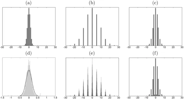
whereq2is the second quantization step andzis the final double quantized DCT coefficient. To illustrate the effect of double quantization, consider an example where the original DCT coefficients are normally distributed in the range [−30,30]. Shown in Figure 4.2(a) is the distribution of these coefficients after being quantized with q1 = 5, Equation (4.1).

(45)

(a) (b) (c)

(d) (e) (f)

Figure 4.2: Shown are: (a) the distribution of singly quantized coefficients withq1 = 5; (b) the

distribution of these coefficients de-quantized; (c) the distribution of doubly quantized coefficients with q1 = 5 followed by q2 = 3 (note the empty bins in this distribution); (d) a magnified view

of the central bin in panel (e) – the dashed line is a Gaussian distribution fit to the underlying coefficients; and (e-f) the same distributions shown in panels (b) and (c) but with rounding and truncation introduced after the coefficients are decoded.

Shown in Figure 4.2(b) is the distribution of the de-quantized coefficients, Equation (4.2) (where every coefficient is now a multiple of the first quantization 5). And shown in Fig-ure 4.2(c) is the distribution of doubly quantized coefficients with stepsq1= 5 followed by

q2 = 3, Equation (4.3). Because the step size decreases fromq1= 5 toq2 = 3 the coefficients are re-distributed into more bins in the second quantization than in the first quantization. As a result, the distribution of the doubly quantized coefficients contains empty bins (Fig-ure 4.2(c) as compared to Fig(Fig-ure 4.2(a)). As described in [34, 43, 18], a similar, although less pronounced, artifact is introduced when the step size increases between quantizations. Since we will be computing double compression artifacts at the level of a single macro-block, we will restrict ourselves to the more pronounced case when q1 > q2.

Modeling Double Quantization

Equations (4.1)-(4.3) describe the effects of double compression in an idealized setting. In practice, however, when a compressed video is de-quantized, Equation (4.2), and an inverse DCT applied, the resulting pixel values are rounded to the nearest integer and truncated

(46)

into the range [0,255]. When the forward DCT is then applied, the coefficients will no longer be strict multiples of the first quantization step. Shown in Figure 4.2(d) is an example of this effect, where only a single bin is shown – note that instead of being an impulse at 0, the coefficients approximately follow a normal distribution centered at zero. Superimposed on this distribution is a Gaussian distribution fit to the underlying coefficients. Shown in Figure 4.2(e) is an example of how the rounding and truncation affect the entire distribution (note the contrast to the ideal case shown in panel (b)). After the second compression, the rounding and truncation are propagated into the doubly quantized coefficients. As a result, the previously empty bins are no longer empty, as shown in Figure 4.2(f), as compared to panel (c).

We therefore model the distribution of singly compressed and de-quantized coefficients with a Gaussian distribution:

Pq1(y|x) = N(y;xq1, σ) =

1

σ√2πe

−(y−xq1)2

2σ2 , (4.4)

with mean xq1 and standard deviationσ. This conditional probability describes the distri-bution of de-quantized coefficients y with respect tox.

The distribution of doubly compressed coefficients is then given by:

Pq1(z|x) = Z (z+0.5)q2 (z−0.5)q2 Pq1(y|x)dy = Z (z+0.5)q2 (z−0.5)q2 N(y;xq1, σ)dy, (4.5)

where the integration bounds mimic the rounding function.

Now, the marginal distribution on the observed doubly compressed coefficientszis given by: Pq1(z) = X x Pq1(x)Pq1(z|x) = X x Pq1(x) Z (z+0.5)q2 (z−0.5)q2 N(y;xq1, σ)dy. (4.6)

(47)

from having been quantized with step sizeq1 followed byq2. Since the second quantization

q2 can be determined directly from the encoded video, this distribution can be used to determine if the observed DCT coefficients are consistent with double compression, where the first compression occurred with quantization q1.

Note that in our model of Pq1(z), Equation (4.6), the marginal probability Pq1(x) that

describes the distribution of the original quantized coefficients is unknown. We next describe how to estimate this unknown distribution.

LetZ ={z1, z2, . . . , zn}denote a set ofnobservations of the DCT coefficients extracted from a single macroblock. Given Z, the distribution Pq1(x) can be estimated using the

expectation-maximization (EM) algorithm [9]. The EM algorithm is a two-step iterative algorithm. In the first E-step the distribution ofxgiven each observationzi is estimated to yield Pq1(x|zi). In the second M-step the distribution of x is computed by integrating the

estimated Pq1(x|zi) over all possiblezi to yield the desiredPq1(x).

More specifically, in the E-step, we estimatePq1(x|zi) using Bayes’ rule:

Pq1(x|zi) =

Pq1(x)Pq1(zi|x)

Pq1(zi)

, (4.7)

wherePq1(zi|x) is given by Equation (4.5) andPq1(zi) is given by Equation (4.6). Note that

this step assumes a knownPq1(x), which can be initialized randomly in the first iteration.

In the M-step,Pq1(x) is updated by numerically integrating Pq1(x|zi) over all possiblezi:

Pq1(x) = 1 n n X i=1 Pq1(x|zi). (4.8)

These two steps are iteratively executed until convergence.

Forensics

Our model of double compression described in the previous section can be used to determine if a set of DCT coefficients have been compressed twice with quantization steps ofq1followed by q2. Let Z denote the DCT coefficients from a single macroblock whose quantization scale factor is q2 (the value of q2 can be extracted from the underlying encoded video).

(48)

LetP(z) denote the distribution ofZ. This distribution can be compared to the expected distributionPq1(z), Equation(4.6), that would arise if the coefficients are the result of double

quantization by stepsq1followed byq2. To measure the difference between the observedP(z) and modeled Pq1(z) distr