Exploring Data Clustering with Non-negative Matrix Factorization Models
A Thesis
Submitted to the Faculty of
Drexel University by
Zunyan Xiong in partial fulfillment of the requirements for the degree
of
Doctor of Philosophy in Information Studies May 2015
ii
Acknowledgements
My deepest gratitude goes to my Ph.D. adivisor, Dr. Xiaohua Hu, who has supported me throughout my thesis with his knowledge, his intuitive vision, and his work ethics, and also given me the freedom to explore on my own. His patience and support helped me overcome many difficult situation and finish this dissertation. Especially when I told him the news of my pregnancy, he congratulated me in the first place, and encouraged me to get prepared for the baby. Without him this thesis would not have been completed or written. One simply could not wish for a better or friendlier supervisor.
A special thanks goes to Prof. Lisa Ulmer, with whom I worked with for three years. During the years of collaboration, she gave me a vivid impression of her intel-ligence, professional and considerateness. She never missed a meeting we scheduled and always came in time. She is such a great project leader that methodically and logically proceeded our progress. Meanwhile, she is kind to all the people around her. In a word, she is strict with herself and broad-minded towards others. How I wish I had never heard the sad news about her on this June. Wish Prof. Lisa Ulmer rest in peace in heaven.
I would also like to thank the rest committee: Prof. Yuan An, Prof. Weimao Ke and Prof. Li Sheng for their time and effort to serve on my dissertation committee, and for their insightful comments on my dissertation and defense, which helped shape this work and my future thinking in this research domain.
My sincere thanks to my labmate and roommate Jia Huang and Xiaoli Song, for the simulating discussions in research, for the sleepless nights we worked together before deadlines, for the weekends we went shopping in grocery stores, and for the days we tidied the rooms together.
pro-vided me with research advice at times of critical need.
I thank my office fellows Xuemei and Mi Zhang for the days we communicated research as well as gossip, we traveled together on cruise, and we enjoyed hot-pot in every winter break.
I appreciate Caimei Lu, Lifan Guo, Xin Chen, and Xuning Tang and Haozhen Zhao for helping me adapt the study and life when I was a fresh PhD student.
I also owe many thanks to my friends Yue Shang, Mengwen Xu, Weiwei Xu, Wanying Ding, Zhan Zhang, Lu Xiao, Ling Jiang and Haodong Yang for all the fun we have had in last several years. Without you, the color of my life in Philly would be much paler.
Last but not the least, I would like to thank my family: my parents and my husband for supporting me spiritually throughout writing this thesis and my life in general. I thank my son, whose coming opens an amazing window for me to see, touch, and feel the world start over with him. That is really a fantastic experience.
iv
Table of Contents
Acknowledgements . . . ii
LIST OF TABLES . . . vi
LIST OF FIGURES . . . viii
ABSTRACT . . . x
1. INTRODUCTION . . . 1
1.1 Clustering and Non-negative Matrix Factorization . . . 1
1.2 The strategies and the outline . . . 3
2. A REVIEW OF DATA CLUSTERING . . . 7
2.1 The kernel K-means . . . 7
2.2 Principal component analysis (PCA) . . . 9
2.3 Topic models . . . 11
2.3.1 Latent semantic analysis (LSA) . . . 13
2.3.2 Probabilistic latent semantic analysis (PLSA) . . . 14
2.3.3 Latent dirichlet allocation (LDA) . . . 15
2.3.4 Comparison of topic models . . . 17
3. A REVIEW OF NON-NEGATIVE MATRIX FACTORIZATION AND ITS EXTENSION . . . 20
3.1 The NMF model . . . 20
3.1.1 Formulation of the model . . . 20
3.1.2 The multiplicative algorithm . . . 20
3.2 Some generalizations of the NMF . . . 22
3.2.1 Symmetric NMF . . . 22
3.2.2 Graph regularized NMF . . . 23
3.2.3 Sparse NMF. . . 24
3.3 Higher dimensions: non-negative tensor factorization (NTF) . . . 25
3.3.1 The PARAFAC model . . . 25
3.3.2 The multiplicative algorithm . . . 27
4. DATA SETS AND EVALUATION METRICS . . . 30
4.1 Data Sets . . . 30
4.2 Evaluation Metrics. . . 31
5. NMF MODELS: CONSTRAINTS VS. REGULARIZATIONS . . . 33
5.1 Introduction . . . 33
5.2 The similarity matrix . . . 34
5.3 NMF models with constrains . . . 36
5.3.1 Problem formulation . . . 36
5.3.2 The Multiplicative algorithm . . . 37
5.4 NMF models with regularizations . . . 38
5.4.1 The Multiplicative algorithm . . . 39
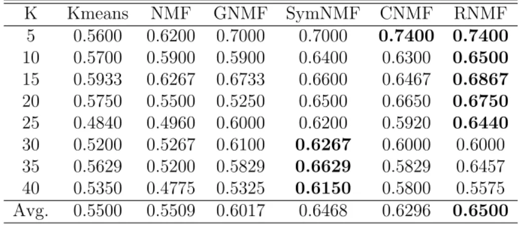
5.5 Experiments . . . 41
5.5.1 Data sets and evaluation metrics . . . 41
5.5.3 Clustering results . . . 42
5.5.4 Sensitivity in relation to parameters . . . 44
6. THE AUGMENTED NMF MODEL . . . 47
6.1 Formulation of the model . . . 47
6.1.1 Notations and set-ups . . . 48
6.1.2 Local invariance assumption . . . 49
6.1.3 Augmented NMF model . . . 51
6.2 Analysis of the algorithm . . . 52
6.2.1 The multiplicative algorithm . . . 52
6.2.2 Complexity analysis . . . 54
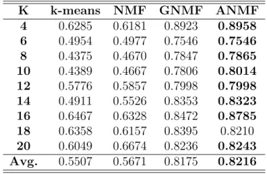
6.3 Experiments . . . 55
6.3.1 Data sets and evaluation metrics . . . 55
6.3.2 Parameter settings. . . 55
6.3.3 Clustering results . . . 56
6.3.4 Sensitivity in relation to parameters . . . 57
6.4 Study on the CiteULike data set . . . 59
6.4.1 Data processing . . . 59
6.4.2 Clustering resluts . . . 61
6.5 The regularized NTF model . . . 63
6.5.1 Local Invariance and Document Similarity . . . 63
6.5.2 Regularized NTF Model . . . 65
6.5.3 A Multiplicative Algorithm . . . 65
6.6 Conclusions. . . 67
7. THE SPARSE REGULARIZED NMF MODEL . . . 68
7.1 Formulation of the model . . . 68
7.1.1 Notations . . . 69
7.1.2 Data graph regularization . . . 69
7.1.3 Sparse graph regularized NMF . . . 70
7.2 Alternating iterative algorithm . . . 72
7.3 Experiments . . . 74
7.3.1 Data sets and evaluation metrics . . . 74
7.3.2 Parameter settings. . . 74
7.3.3 Clustering results . . . 75
7.3.4 Sensitivity in parameters . . . 77
7.4 Conclusion. . . 78
8. CONCLUSION AND FUTURE WORKS . . . 80
BIBLIOGRAPHY . . . 83
vi
List of Tables
2.1 The algorithm for K-means. . . 8
3.1 The NMF algorithm . . . 22
3.2 The PARAFAC algorithm . . . 29
4.1 Description of Experimental Data Sets . . . 31
5.1 The algorithm for constrained NMF . . . 38
5.2 The algorithm for regularized NMF . . . 40
5.3 Performance comparisons of CNMF & RNMF on Yale: Acc . . . 43
5.4 Performance comparisons of CNMF & RNMF on Yale: NMI . . . 43
5.5 Performance comparisons of CNMF & RNMF on ORL: Acc. . . 44
5.6 Performance comparisons of CNMF & RNMF on ORL: NMI. . . 44
6.1 Important notations used in this chapter. . . 48
6.2 Algorithm of ANMF. . . 55
6.3 Performance comparisons of ANMF on Coil20: Acc . . . 57
6.4 Performance comparisons of ANMF on Coil20: NMI . . . 58
6.5 Performance comparisons of ANMF on ORL: Acc . . . 58
6.6 Performance comparisons of ANMF on ORL: NMI . . . 59
6.7 Performance comparisons of ANMF on TDT2: Acc . . . 59
6.8 Performance comparisons of ANMF on TDT2: NMI . . . 60
6.9 Performance comparisons of ANMF on Reuters21578: Acc . . . 60
6.11 The Acc performance of ANMF in CiteULike data set . . . 62
6.12 The NMI performance of ANMF in CiteULike data set . . . 63
7.1 Important notations used in this chapter. . . 69
7.2 The SpaNMF algorithm . . . 73
7.3 Performance comparisons of SpaNMF on Yale: Acc . . . 76
7.4 Performance comparisons of SpaNMF on Yale: NMI . . . 76
7.5 Performance comparisons of SpaNMF on ORL: Acc . . . 77
viii
List of Figures
1.1 Data clustering. [39] . . . 3
2.1 An example of the clustering using K-means. Data points are denoted by dots and the centroid of two clusters are denoted by ×simbol. The Figure is due to Michael Jordan. . . 9
2.2 The dashed lines represents the decomposed principal components. The dots represents original data. Figure taken from [1].. . . 10
2.3 Probabilistic Latent Semantic Model. . . 18
2.4 Latent Dirichlet Allocation Model . . . 18
2.5 Geometric Interpretation of Topic Models . . . 19
5.1 The performance of CNMF varies with the size of neighborhood pin Yale (left) and ORL (right) data sets. . . 45
5.2 The performance of RNMF varies with the size of neighborhood pin Yale (left) and ORL (right) data sets. . . 46
5.3 The performance of RNMF varies with the regularization parameter β in Yale (left) and ORL (right) data sets. . . 46
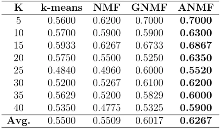
6.1 The performance of ANMF varies with the size of neighborhoodpin Coil20 (left) and ORL(right). . . 61
6.2 The performance of ANMF varies with γ in Coil20 (left) and ORL(right). . 62
6.3 The performance of ANMF varies with δ in Coil20 (left) and ORL(right). . 62
7.1 The performance of SpaNMF varies with the size of neighborhood p in Yale (left) and ORL (right) data sets. . . 78
7.2 The performance of SpaNMF varies with the regularization parameter λ. The left figure is for Yale with µ= 100. The right is for ORL with µ= 0.1 79 7.3 The performance of SpaNMF varies with the regularization parameter µ. The left figure is for Yale with λ = 1. The right is for ORL withλ= 1. . . 79
8.1 The accumulative performance comparison of ALL NMF models using Yale data set. . . 81
8.2 The accumulative performance comparison of ALL NMF models using
x
Abstract
Exploring Data Clustering with Non-negative Matrix Factorization Models Zunyan Xiong
Advisor: Xiaohua Hu, Ph.D.
The clustering problem has been widely studied in data mining and machine learn-ing. It has numerous applications to pattern recognition, information retrieval, image analysis and bioinformatics, etc. In general, clustering is a fundamental unsupervised machine learning technique that aims to partition the data set based on their sim-ilarity. Recently there has been significant development in the use of non-negative matrix factorization (NMF) methods for various clustering tasks. The method finds two negative matrix whose product approximates the original matrix. The non-negativity of the factored matrices is superior to other matrix factorization methods because it makes the data interpretation much easier. Moreover, NMF has attracted much attention due to the newly discovered ability of solving challenging data mining and machine learning problems. Studies has proved that NMF is equivalent with kernel k-means and probabilistic latent semantic indexing under some circumstances. Compared to most other clustering methods, NMF has been proved to achieve better or similar clustering results.
In the thesis, our primary goal is to study the clustering problem by establish-ing NMF models reflectestablish-ing the features of given data. First, in the case when the similarity of the data is available, we proposed two modified NMF models, one with a constraint (CNMF) and the other with a regularization term (RNMF). We take this situation as an example to show how to model the data information. Also, we compare the two commonly employed approach in this simple case. Next, we pro-pose a novel model named augmented nonnegative matrix factorization (ANMF).
The novelty of the model is that it incorporates the geometric closeness of the data on both dimensions of the data matrix. In addition to the experiments conducted on benchmark data sets, the model is also applied to real application, i.e. CiteUlike data set. Finally, for data sets with sparse features, we propose a new model named sparse regularized non-negative matrix factorization (SpaNMF). This type of data is ubiquitous in applications and has remained a hot topic for many years. Our novelty here is to combine the geometric structure and sparseness of the data. For all of the four models, we develop numerical algorithms and conduct the experiments. The results of the experiments show effectiveness of our proposed models compared with state-of-the-art clustering algorithms.
1. INTRODUCTION
1.1 Clustering and Non-negative Matrix Factorization
Clustering has been considered as a core task in data mining [33], which aims to partition a data set into clusters based on their similarity. Intuitively, the data within a cluster are expected to be more similar to each other than the data belonging to a different cluster. An example of clustering is depicted in Figure 1.1. Figure 1.1(a) shows the input data set, and Figure 1.1(b) shows the desired clusters, where points belonging to the same cluster are given the same label.
Clustering and classification are often mentioned together in literature, it is note-worthy to understand their differences. Classification is also called supervised learning method, which means the training set of data are provided with category labels, and the problem is to give new comers the “right” labels. Typically, the labeled data are used to learn the features of the classes, which in turn are used to label new data. Clustering is an unsupervised machine learning method, which means no category labels are given before grouping data, so there is no unique “right” answer for clus-tering results, and the category labels have to be explored solely from the data. As the notion of “cluster” cannot be precisely defined, that’s also one of the reason why there are so many clustering methods [23].
Clustering has been extensively applied in a large variety of fields, such as pattern recognition [2][22][40], image processing[11][83][74][61], recommender system [67][53][43], and information retrieval [41][51][72]. So far clustering also have been widely explored in data mining area, such as k-means [38], spectral clustering [6], nonnegative matrix factorization (NMF) ([55]), etc.
2 of the factorized matrices. Compared to most other clustering methods, it has been proved to achieve better or similar clustering results. NMF aims to approximate the original matrix by the production of the two factorized nonnegative matrices, which is superior for straightforward interpretation. Though as a dimension reduction method, NMF has received much attention for its application to data clustering. [77] firstly applied NMF in document clustering using term-document matrix, the experimental evaluations of NMF outperformed the latent semantic indexing and the spectral clustering methods. [79] applied NMF in topic learning by exploring term correlation data. [66] applied an extended NMF models in image clustering. [9] and [47] successfully applied NMF to biological data.
Notwithstanding that NMF have produced so many good clustering results, as a dimension reduction method, NMF doesn’t always achieve the best clustering results. For instance, NMF considers clusters linearly dependent, while in reality, quite a lot of data have nonlinear cluster structures. In [12], Cai et al. proposed a graph regular-ized non-negative matrix factorization (GNMF), which embedded manifold learning into nonnegative matrix factorization by means of local invariance assumption. [26] combined graph regularization with NMF and applied the model in text clustering. [32] proposed a dual regularized co-clustering method, which applied graph regular-ization in both dimensions of a data matrix. All the above mentioned methods proved the applying graph/manifold regularization can significantly improve the clustering results. In some other cases, a sparser basis or representation are expected after the matrix factorization. Kim and Park used a sparsity constrained NMF and analyzed gene expression data [47].
Although clustering has been extensively studied by researchers in different areas, so far it’s still a challenging problem. One challenge is that given the little prior information about the data, people has to make appropriate assumption about the
data during the building process of clustering models [39]. That’s where lies the advantage of NMF models, i.e., one can easily translate the prior information of the data into the assumption about the model, and build a clustering model that may best fit the real data structure. In this thesis, our main research question is: given by the prior information of the data set, how to achieve a good clustering result by customizing NMF models? In the next section, we will introduce our strategies in detail.
methods for grouping of unlabeled data. These communities have different ter-minologies and assumptions for the components of the clustering process and the contexts in which clustering is used. Thus, we face a dilemma regard-ing the scope of this survey. The produc-tion of a truly comprehensive survey would be a monumental task given the sheer mass of literature in this area. The accessibility of the survey might also be questionable given the need to reconcile very different vocabularies and assumptions regarding clustering in the various communities.
The goal of this paper is to survey the core concepts and techniques in the large subset of cluster analysis with its roots in statistics and decision theory. Where appropriate, references will be made to key concepts and techniques arising from clustering methodology in the machine-learning and other commu-nities.
The audience for this paper includes practitioners in the pattern recognition and image analysis communities (who should view it as a summarization of current practice), practitioners in the machine-learning communities (who should view it as a snapshot of a closely related field with a rich history of well-understood techniques), and the broader audience of scientific
profes-sionals (who should view it as an acces-sible introduction to a mature field that is making important contributions to computing application areas).
1.2 Components of a Clustering Task
Typical pattern clustering activity in-volves the following steps [Jain and Dubes 1988]:
(1) pattern representation (optionally including feature extraction and/or selection),
(2) definition of a pattern proximity measure appropriate to the data do-main,
(3) clustering or grouping,
(4) data abstraction (if needed), and (5) assessment of output (if needed). Figure 2 depicts a typical sequencing of the first three of these steps, including a feedback path where the grouping process output could affect subsequent feature extraction and similarity com-putations.
Pattern representation refers to the number of classes, the number of avail-able patterns, and the number, type, and scale of the features available to the clustering algorithm. Some of this infor-mation may not be controllable by the
X X Y Y (a) (b) x x x x x 1 1 1 x x 1 1 2 2 x x 2 2 x x x x x x x x x x x x x x x x x x x 3 3 3 3 4 4 4 4 4 4 4 4 4 4 4 4 4 44 x x x x x x x x 6 6 6 7 7 7 7 6 x x x x x x x 4 5 55 5 5 5
Figure 1. Data clustering.
266 • A. Jain et al.
ACM Computing Surveys, Vol. 31, No. 3, September 1999
Figure 1.1: Data clustering. [39]
1.2 The strategies and the outline
In this work, our primary goal is to study the clustering problem by establishing models reflecting the features of given problems. As shown in previous researches, the clustering results are improved by properly identifying the structure and main features of the data. For example, the sparseness, the manifold structure, etc. This motivates our study. From another point of view, these data features can be regarded as a way to select a better solution to the optimization problem of a clustering model
4 when the solution is not unique.
Our strategy is that for particular problems, we first explore the data structure and extract useful information. Then we build new models by including these information. For the first part, we explore the data structure from some geometrical and statistical aspects. The basic model we use is the non-negative matrix factorization (NMF), which has been widely applied in data mining. To model the extra information, we use the regularization technique in general. This means after quantifying the extra information, we formulate it as a regularization term to the cost function of NMF. We develop multiplicative algorithms for each model we build, and we discuss the effectiveness of our models compared with the state-of-the-art models.
The main contribution and novelty of this work, as explained below in detail, is to systematically study the NMF model with regularization terms reflecting data structures, and prove their effectiveness. In general , when the similarity of the data is known, we formulated two mathematic models, i.e. CNMF and RNMF (see be-low), which are shown to be superior with state-of-the-art algorithms. For two cases, when other data features are better understood (geometric structure or sparseness), we proposed two regularized NMF models (the ANMF and SpaNMF discussed be-low) which are illustrated to be more effective compared to previous works. These researches confirm our point of view that to achieve better clustering results, it is necessary to include the data features to a given clustering problem. Moreover, the methodologies proposed in this work are expected to be useful for other clustering problems.
Next we outline the contents of this work.
In Chapter 2, we briefly review some widely used clustering methods, including K-means, principal analysis and topic models. In particular, we emphasis their relations to matrix factorization methods. Actually, most of these methods can be interpreted
as matrix factorizations e.g. singular value decomposition and NMF. Since we use NMF extensively, we review them in Chapter 3 in more details. Here we formulate the NMF models following the classic work of Lee and Seung [55] and derive its multiplicative algorithms. These preparations will be quite useful for our models developed later. Also, we review some generalized NMF models which also explores the data structures.
In Chapter 4, we introduce some standard data sets applied in this thesis. Our intention is to emphasize some useful features of the data which will be explored later. Also, we discuss the evaluation metrics for experiments.
Next, in Chapter 5, we start with a simple situation where we are given the similarities of the data. We discuss two ways to model this information i.e. regarding it as a constraint to the optimization problem or a regularization term. The obtained two models are called CNMF and RNMF respectively. Our intention is to take this situation as an example to show how to model the data information. Also, we’d like to compare the two commonly employed approach in this simple case. For both models, we derive multiplicative algorithms. Finally, we test and compare the methods using standard data.
In Chapter 6, based on the GNMF method proposed by Cai et al [12], we develop a new augmented NMF model, the Augmented NMF model(ANMF). The novelty of our model is that we use geometric structure of the data in both dimensions (compared to one dimension in Cai et al [12]) to get the extra information. In particular, we use the so-called local invariance which roughly speaking says that the similarity of the data should be preserved after the decomposition. We derive the multiplicative algorithm, and test its effectiveness. Finally, we applied the new model to real applications, i.e. CiteULike data set. Also, we discuss the generalization to higher dimensional data i.e. tensors.
6 In Chapter 7, we develop a new model for data set with sparseness, called SpaNMF. This type of data is ubiquitous in applications and has remained a hot topic for many years. There are some pioneering work in the sparseness of NMF models. However, our novelty here is to combine the geometric structure and sparseness of the data. In particular, we develop a sparse regularized model in Chapter 6 which include two regularization terms, one reflecting the local invariance and the other reflecting the sparseness. We are able to derive the multiplicative algorithm without burdening the computational cost too much. The experiments also show the effectiveness of our model.
In Chapter 8, we make a general review of the four proposed NMF models: CNMF, RNMF, ANMF and SpaNMF. Finally, we make comments on future research topics.
2. A REVIEW OF DATA CLUSTERING
2.1 The kernel K-means
Despite its simplicity, the kernel K-means method is widely used in clustering problems. As discussed by Kuang et al [46], the method is also related to the matrix factorization models. In this section, we review the basics of the model and its algorithm.
Consider a set of data {x1, x2,· · · , xN}where eachxi is a vector inRM. We’d like
to group the data to K clustersCk, k = 1,2,· · · , K. The K-means method make use
of the centroid of the clusters as a characterization of the cluster class. In particular, suppose there are nk data points in Ck. Let
mk = X i∈Ck
xi/nk
be the centroid of the cluster Ck. The objective function of K-means is
OK = K X k=1 X i∈Ck kxi−mkk2.
Here k · k denotes the Euclidean norm of a vector. The optimization problem is to find Ck which minimizes OK.
The algorithm for K-means is easy to state and summarized in Table ??. See
Figure 2.1 for an example of the clustering precedure. In particular, in the first step of the loop, we determine the cluster number for each xi. The second step compute
the new centroid. The algorithm converges in the sense that it decreases the objective function after each iteration, see e.g. Lecture notes of Ng [60].
8 Table 2.1: The algorithm for K-means.
1. Randomly initialize the centroid m1, m2,· · · , mK;
2. Repeat
Step a : For every i, set ci = argminkkxi−mkk2;
Step b : For each k, set mk =Pci=kxi/Pci=k1.
until convergence.
factorization models which we discuss in detail in Chapter 3. For later reference, we reformulate the objective functionOK. From the straightforward calculation, we have
OK = N X i=1 kxik2− K X k=1 1 nk X i,j∈Ck xTi xj.
The solution of the clustering result can be represented by vectors
H = (h1, h2,· · · , hK),
where hk is a vector in RN such that
hTi hj =δij and nkhTk = (0,· · · ,0,1,· · · ,1,· · · ,0),
where the number of 1’s in the vector is nk. In other words, hk is an indicator of the
cluster Ck i.e. xi ∈Ck if and only if (hk)i = 0. Let6 H = [h1, h2,· · · , hK] be a N ×K
dimensional matrix and X = [x1, x2,· · · , xN] be a M×N dimensional matrix. Then
OK can be written as
OK = Tr(XTX)−Tr(HTXTXH).
(a) (b) (c)
(d) (e) (f)
Figure 1: K-means algorithm. Training examples are shown as dots, and cluster centroids are shown as crosses. (a) Original dataset. (b) Random ini-tial cluster centroids (in this instance, not chosen to be equal to two training examples). (c-f) Illustration of running two iterations of k-means. In each iteration, we assign each training example to the closest cluster centroid (shown by “painting” the training examples the same color as the cluster centroid to which is assigned); then we move each cluster centroid to the mean of the points assigned to it. (Best viewed in color.) Images courtesy Michael Jordan.
Is the k-means algorithm guaranteed to converge? Yes it is, in a certain sense. In particular, let us define the distortion functionto be:
J(c, µ) =
m X
i=1
||x(i)−µc(i)||2
Thus,J measures the sum of squared distances between each training exam-ple x(i) and the cluster centroid µ
c(i) to which it has been assigned. It can
be shown that k-means is exactly coordinate descent on J. Specifically, the inner-loop ofk-means repeatedly minimizesJ with respect tocwhile holding
µfixed, and then minimizes J with respect toµwhile holding cfixed. Thus,
J must monotonically decrease, and the value of J must converge.
(Usu-ally, this implies that c and µ will converge too. In theory, it is possible for Figure 2.1: An example of the clustering using K-means. Data points are denoted by dots and the centroid of two clusters are denoted by× simbol. The Figure is due to Michael Jordan.
gives the cluster result. We remark that this formulation is closely related to the Symmetric NMF method as demonstrated in [21].
2.2 Principal component analysis (PCA)
The principal component analysis belongs to the broad family of dimensionality reduction methods, see e.g. Ghodsi [28]. Generally speaking, the idea is to de-compose high dimensional data to low dimensional representations. We review the PCA method not only because its wide usage in applications, but also because its key mathematical model involves an important matrix factorization technique: the singular value decomposition (SVD).
10 tune the parameters without knowing the distribution of the data in advance. This suggests that statistical models might be able to better describe the data, assuming an underlying probability distribution. An algorithm that iteratively estimates the distribution of the data is described in Section5.2.
The difference between the Fuzzy Codok algorithm and that of Section7.3should be pointed out. On face value, both generate fuzzy memberships for documents and terms. However, while Fuzzy Codok employs a notion of aggregation in the original feature space, the latter employs PCA techniques, described next, and works in a reduced space resulting from matrix factorization.
7
Dimensionality Reduction
While proprocessing can achieve significant reduction in the size of the vector space, post-retrieval appli-cations call for higher efficiency. This section describes describes two matrix factorization techniques that have been shown to not only significantly reduce the size of document vectors (by several orders of magni-tude), but also to increase clustering accuracy. In fact, these methods can be viewed as clustering methods themselves (although post-processing is required in the case of spectral coclustering, see Section7.1).
The remainder of this section assumes a term-document matrixA∈Rm+×n. The goal of dimensionality reduction techniques is to produce a rankkapproximation of A,Ak, while introducing managable error. A common measure of the quality of this approximation is the Frobenius norm, which is defined as
|A−Ak|= sX a∈A X ak∈Ak (a−ak)2 (21)
The smaller the Frobenius norm, the better the matrixAk approximates the original matrixA.
7.1 Principal component analysis
Principal components are orthogonal (i.e. uncorrelated) projections that together explain the maximum amount of variation in a dataset. In practice, principle components can be found by computing the singular value decomposition on the correlation matrix of the dataset. This method is sometimes called spectral projection. This is illustrated in Figure7.
Figure 7: The two dashed lines represent principal components capturing the variability in the dataset. The singular value decomposition of the original matrixAinvolves breaking it up into the matrices:
An≈UΣVT (22)
14
Figure 2.2: The dashed lines represents the decomposed principal components. The dots represents original data. Figure taken from [1].
matrix which possesses eigenvalues, the spectral data of A is the singular value. We know thatATA is symmetric and denote its eigenvalues by λ
1, λ2,· · · , λn ordered by
their magnitudes. The singular values of A is the set {√λ1,
√
λ2,· · · ,
√
λn}.
More-over, we can find two orthogonal matrices U ∈Rm×m and V ∈Rn×n so that
A=UΣV,
where Σ ∈Rm×n with diagonal elements the singular values. Intuitively, we
decom-posedAto some linear spaces with the significance represented by the singular values. See Figure 2.2.
To get an approximation of A, we can truncate Σ to Σk by keeping the first k
singular values. We get
Ak=UΣkV,
and we use Ak as an approximation to A. According to the construction, Ak has
method. The vectors ofU can be used for document clustering see e.g. [81].
As reviewed in [1], PCA has two properties especially convenient for clustering: approximation and distinguishability, see also [73]. It is proved in [20] that the prin-cipal component are also the solutions to K-means. However, the computational cost of SVD for large matrices is expensive and it cannot be performed in an iterative way. In particular, PCA is not an optimization problem. A major problem for PCA is that the decomposed matrices may have negative values, which makes it hard to explain the meaning of the decomposed data. Actually, the major advantage of the non-negative matrix factorization method which we review in the next chapter is the non-negativity of the decomposed values.
2.3 Topic models
Topic models form a large class of clustering methods which involves numerous research activities. Usually, these models are built using statistical method and some-times they are related to matrix factorization. We review some of the classical models here as a comparison to matrix factorization models.
In general, topic models aim at discovering abstract “topics” in the document corpus. According to [64], topic models are based on the idea that the topics of documents can be represented by probability distribution of topics, and each topic is a mixture of words. Bearing the idea, topic models are considered promising in solving synonymy and polysemy problems. With the induction of the conception of abstract “topic”, topic models can put words with similar semantic meanings together, thus alleviate the synonymy problem. On the other hand, a word with different meanings may belong to different topics, which improve the performance of the system on polysemy problem. In addition, topic models take into account the co-occurrence of words, which provide better understanding to the semantic structure of text corpus.
12 Topic models have been intensively studied since 1990s of last century. In order to approximate the real semantic patterns from unstructured data set, researchers have explored different methods to extract abstract “topics” from documents. And different approaches have also been applied to estimate parameters in text corpus.
Topic models can be applied in various areas, such as text classification [5], im-age annotation [5], imim-age classification [24], joint modeling the patterns of the text and citations [59], real-time tag recommendation [70], etc. Cohn and Hofmann [16] integrate content and inter-association of documents in PLSA model. PSLA model identifies major topics of the collections and prominent document in the documents. In addition to the probability distribution among words, they applied hyperlinks or citations between documents to explore the associations between topics.
Rosen-Zvi et al. [62] introduce author-topic model based on Latent Dirichlet Al-location model. In author-topic model, each author is connected with a multinomial distribution over topics and each topic is a multinomial distribution over words. A document with authors is a distribution over topics which are a mixture of distribu-tions related with the authors. Gibbs sampling is applied to estimate the distribution of topics and words. Liu et al. [54] propose a topic-link LDA model to identify both research community and major topics from articles. They posit that documents are not only connected by the content similarity, they are also connected by the social ties between the authors. The connection between documents is represented by a binomial distribution modeled by the similarity between topic distribution and com-munity distribution and also a random factor. Variational EM algorithm is applied to estimate parameters.
2.3.1 Latent semantic analysis (LSA)
Latent Semantic Analysis (LSA, also refers to Latent Semantic Indexing, LSI) is proposed by Scott Deerwester and his collaborators in 1990. It assumes that docu-ments which contain frequently co-occurring terms will have similar semantic pattern, even if they have no terms in common [36]. The core of LSA is singular value decom-position (SVD) which reduces the dimension of data structure. The authors assert that after singular value decomposition, both terms and documents can be mapped in the compressed space. Besides, the arrangement of the space can reflect the major connected patterns in the data set, and the trivial influences would be dismissed.
The process of LSA starts with a term-document matrix X that based on term frequencies. Then it applies SVD to decompose the matrix into left and right singular vectorsU andV, and also a diagonal matrix of singular values Σ [19]. MatrixXcan be expressed by X =UΣV∗, where U and V are orthogonal matricesU U∗ =V∗V =I. After SVD, all the vectors are independent / orthogonal to each other. SVD can be viewed as a method for generating a set of independent factors. Each term and document is described by its vector of factor values [19]. Here, the independent factors can be viewed as abstract “topics”.
Compared to traditional TF-IDF method, LSA can significantly compress large collection. Besides, it can make terms that absent in a document close to the docu-ment in the space, if they are consonant with the key patterns of relationship in the data.
However, the author admitted that the model of latent semantic indexing is weaker in dealing with polysemy though competitive in solving synonymy problem [19]. Be-sides, the statistical foundation of LSA is also not convincing [5], [36]. These deficits led to the emergence of probabilistic Latent Semantic Analysis.
14
2.3.2 Probabilistic latent semantic analysis (PLSA)
Thomas Hofmann proposed Probabilistic Latent Semantic Analysis (PLSA) in 1999. Unlike the LSA model, which is based on the theory of linear algebra, the core of PLSA is a statistic model derived from aspect model [37]. PLSA introduce probabilistic principle into topic models, and many of following topics models are statistic models, including Latent Dirichlet Allocation model that will be introduced later. In PLSA, “topics” are represented as multinomial random variables of a mixture model. Each word in a document is regarded as a sample from the mixture model. Thus, each document is represented as the probabilistic distribution of the “topics”. This distribution represents the “reduced description” of the document [36]. In this model, the probability of modeling a word w from a document d can be represented in the expression: P(w|d) = T X z=1 P(w|d)P(z|d).
Hofmann applied Expectation Maximization (EM) algorithm to estimate the max-imum likelihood of latent variable model. EM algorithm contains two steps: one is Expectation (E) step which calculates posterior probabilities for latent variable z, based on current estimates of the parameters; the other is Maximization (M) step which updates parameters for the posterior probabilities that calculated in previous E-step [36].
Compared to LSA, PLSA has the following advantages: (1) It allows the combi-nation of different models. In [36], Hofmann investigated two schemes, PLSI-U and PLSI-Q. The former combines PLSA probability estimates of P(w|d) for the models with different factors T with the same weights; and the latter combines the cosine score of the models. Results from experiments showed that combined model have better performance than the best single model. But in LSA, different factors would
form a nested sequence. (2) PLSA can better deal with polysemous words [36] be-cause in PLSA, a word can be assigned to different topics based on the probability, but a word only has one position in the factor space in LSA.
Although PLSA performs better than LSA [36] and overcomes its problems suc-cessfully; it still has several constraints. In PLSA, each document is represented as a probability distribution of “topics”; the distribution is empirically estimated from ob-served document collection. Therefore, it doesn have a generative probabilistic model for the probability distribution of “topics”. This may cause several problems. First, when the size of the corpus expands, the number of “topics” would also grow, which may cause overfitting problem [5]. Second, when new document or query fold-in, the model needs to be re-estimated onP(z|q) in each M-step of EM algorithm [36], which is not computationally efficient.
2.3.3 Latent dirichlet allocation (LDA)
David M. Blei and his collaborators proposed Latent Dirichlet Allocation (LDA) model in 2003. Similar with PLSA model, LDA is a statistic model, and the “topics” of a document are represented as probabilistic distribution over words, also a docu-ment is a probabilistic mixture of the topics. However, as docu-mentioned in 2.2, PLSA doesn treat the generation of “topics” in a document as a random process. Blei et al. extended the model by adding a Dirichlet prior on θ, which is a multinomial distribution over topics. Besides, LDA have two hyperparameters α and β. α is a
T-dimensional vector with components αi >0 , and β is a T ×N matrix where
βij =p(wj = 1|zi = 1).
Blei et al. assume that the components of the Dirichlet distribution is “known and fixed” [5]. And the word probabilities are also viewed as fixed [5]. The reason for
16 applying Dirichlet distribution in LDA model is that it is conjugate to the multinomial distribution [5] which is convenient for data approximation. Besides, its dimension is sufficient to represent significant pattern of large data collection [5].
The expression of the probability density of a T dimensional distribution on the multinomial distribution p= (p1, p2,· · ·, pT) is:
Dir(α1, α2,· · · , αT) = Γ(Pjαj) Q jΓ(αj) T Y j=1 pαj−1 j .
Similar with PLSA, Blei et al. applied EM algorithm to estimate α andβ param-eters.
Griffiths amd Steyvers [31] (Han, Kamber, and Pei 2006) explored another scheme of LDA model by adding a symmetric Dirichlet φ(β). For each word w, a topic z is chosen from the distributionφ. And for each documentd, a multinomial distribution
θ over topics is sampled from a Dirichlet distribution with the hyperparameter α. The two hyperparmeters α and β can be viewed as the observed frequency of topic
j in a document and the observed frequency of word w in a topic respectively [64]. Different from Blei et al, Griffiths and Steyvers don estimate the distribution ofθ and
φdirectly, instead it estimates the posterior distribution ofp(z|w) first, then estimate
θ and φ according to the posterior distribution.
To estimate the posterior distribution of p(z|w), Griffiths and Steyvers applied Gibbs Sampling algorithm in the model, which significantly relaxes the process of estimation. Gibbs sampling is based on a simple assumption: the joint probability distribution can be approximate by sequentially “sampling each variable from the distribution of that variable on all other variables, making use of the most recent values and updating the variable with its new value as soon as it has been sampled.” [29]
not treat a document as a multinomial random distribution of topics, making it unnatural to fold-in new document. LDA adds the assumption. It generates the topic distribution with a randomly chosen parameter, which is sampled once per document. This method makes new documents be generatively incorporated, and doesn need to re-estimate the entire topic distribution again. (2) The first advantage of LDA also contributes to its scalability. The time needed for estimating parameters will not grow with the expansion of the training corpus.
2.3.4 Comparison of topic models Graphical model perspective
To get a more intuitive vision on topic models, one popular way is applying plate notion of graphical model. A graphical model is a probabilistic model to describe the conditional independence structure between random variables [30]. The plate notions of the three topic models PLSA and LDA models are provided below in Figure 2.5 and Figure 2.3. Note that LSA is not a probabilistic model, so it not depicted by graphical model.
In the plate notions, grey and white circles refer to observed and unobserved (i.e., latent) variables respectively. An arrow indicates a conditional dependency between variables. Variables in the lower right corner of plates are the number of samples, which indicate the repetitions of sampling steps [10]. As mentioned in Section 2, M
and N represent the number of documents and the number of words in the corpus
respectively.
Figure 2.3 shows the plate notion of PLSA model. There are two conditional
dependency relationships. Document d is conditional dependent on topic z, and
topic z is conditional dependent on word w. The estimation of topic distribution on documents requires M repetitions, and the estimation of word distribution on topic
18 requires N repetitions.
can be approximate by sequentially “sampling each variable from the distribution of that variable on all other variables, making use of the most recent values and updating the variable with its new value as soon as it has been sampled.” [8]
Compared to PLSA, LDA has the following advantages: (1) PLSA model does not treat a document as a multinomial random distribution of topics, making it unnatural to fold-in new document. LDA adds the assumption. It generates the topic distribution with a randomly chosen parameter, which is sampled once per document. This method makes new documents be generatively incorporated, and doesn’t need to re-estimate the entire topic distribution again. (2) The first advantage of LDA also contributes to its scalability. The time needed for estimating parameters will not grow with the expansion of the training corpus.
3. COMPARING TOPIC MODELS FROM
DIFFERENT PERSPECTIVES
3.1 Graphical Model Perspective
To get a more intuitive vision on topic models, one popular way is applying plate notion of graphical model. A graphical model is a probabilistic model to describe the conditional independence structure between random variables [10]. The plate notions of the three topic models – PLSA and LDA models – are provided below in Figure 1 and Figure 2. Note that LSA is not a probabilistic model, so it’s not depicted by graphical model. In the plate notions, grey and white circles refer to observed and unobserved (i.e., latent) variables respectively. An arrow indicates a conditional dependency between variables. Variables in the lower right corner of plates are the number of samples, which indicate the repetitions of sampling steps [11]. As mentioned in Section 2, M and N represent the number of documents and the number of words in the corpus respectively.
Figure 1 shows the plate notion of PLSA model. There are two conditional dependency relationships. Document d is conditional dependent on topic z, and topic z is conditional dependent on word w. The estimation of topic distribution on documents requires M repetitions, and the estimation of word distribution on topic requires N repetitions.
Figure 2 describes the plate notion of LDA model. According to Blei et al. [2], 𝛼 and 𝛽 are corpus-level parameters that would be sampled once during the process of creating a corpus. 𝜃 is document-level variables, which would be processed once per document. Variables z and w are word-level variables, which would be sampled once per word in each document.
Figure 1. Probabilistic Latent Semantic Model [2]
Figure 2. Latent Dirichlet Allocation Model [2]
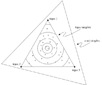
3.2 Geometric Perspective
In [2], Blei et al. compare PLSA model and LDA model and one other model with geometric graph (Figure 3). Here we only introduce the geometric perspective of PLSA model and LDA model. In the graph, there are three topics with three words representing each topic respectively. The topic simplex is contained in the word simplex. And the corners of the word simplex represent the three distribution of each word with probability one [2]. For PLSA model, it places each document on the topic simplex denoted by x with an empirical distribution [2]. While LDA sets each document on the topic simplex represented by the contour lines [2].
Figure 3. Geometric Interpretation of Topic Models [2]
3.3 Other Perspectives
3.3.1 Assumption
1. “Bag-of-Word” assumption. All the three topic models are based on the assumption that the sequence of words in a document can be neglected. In LSA, terms are represented in a term-document matrix, the method only count frequencies of co-occurrence of terms, the order of the words will not affect SVD method. In PLSA, it assumes that the observed (𝑑, 𝑤) pairs are generated independently; this assumption is consistent with “bag-of-words” notion. LDA model is based on randomly assignment of a word to a topic, and randomly selecting topic distribution to a document, which doesn’t take into account the order of words. Also Gibbs sampling doesn’t require a priori order of topics. 2. Both PLSA and LDA assume that each topic is a multinomial distribution over words. But LDA also assumes that each
Figure 2.3: Probabilistic Latent Semantic Model.
Figure 2.5 describes the plate notion of LDA model. According to Blei et al. [5],
α and β are corpus-level parameters that would be sampled once during the process of creating a corpus. θ is document-level variables, which would be processed once per document. Variables z and w are word-level variables, which would be sampled once per word in each document.
can be approximate by sequentially “sampling each variable from the distribution of that variable on all other variables, making use of the most recent values and updating the variable with its new value as soon as it has been sampled.” [8]
Compared to PLSA, LDA has the following advantages: (1) PLSA model does not treat a document as a multinomial random distribution of topics, making it unnatural to fold-in new document. LDA adds the assumption. It generates the topic distribution with a randomly chosen parameter, which is sampled once per document. This method makes new documents be generatively incorporated, and doesn’t need to re-estimate the entire topic distribution again. (2) The first advantage of LDA also contributes to its scalability. The time needed for estimating parameters will not grow with the expansion of the training corpus.
3. COMPARING TOPIC MODELS FROM
DIFFERENT PERSPECTIVES
3.1 Graphical Model Perspective
To get a more intuitive vision on topic models, one popular way is applying plate notion of graphical model. A graphical model is a probabilistic model to describe the conditional independence structure between random variables [10]. The plate notions of the three topic models – PLSA and LDA models – are provided below in Figure 1 and Figure 2. Note that LSA is not a probabilistic model, so it’s not depicted by graphical model. In the plate notions, grey and white circles refer to observed and unobserved (i.e., latent) variables respectively. An arrow indicates a conditional dependency between variables. Variables in the lower right corner of plates are the number of samples, which indicate the repetitions of sampling steps [11]. As mentioned in Section 2, M and N represent the number of documents and the number of words in the corpus respectively.
Figure 1 shows the plate notion of PLSA model. There are two conditional dependency relationships. Document d is conditional dependent on topic z, and topic z is conditional dependent on word w. The estimation of topic distribution on documents requires M repetitions, and the estimation of word distribution on topic requires N repetitions.
Figure 2 describes the plate notion of LDA model. According to Blei et al. [2], 𝛼 and 𝛽 are corpus-level parameters that would be sampled once during the process of creating a corpus. 𝜃 is document-level variables, which would be processed once per document. Variables z and w are word-level variables, which would be sampled once per word in each document.
Figure 1. Probabilistic Latent Semantic Model [2]
Figure 2. Latent Dirichlet Allocation Model [2]
3.2 Geometric Perspective
In [2], Blei et al. compare PLSA model and LDA model and one other model with geometric graph (Figure 3). Here we only introduce the geometric perspective of PLSA model and LDA model. In the graph, there are three topics with three words representing each topic respectively. The topic simplex is contained in the word simplex. And the corners of the word simplex represent the three distribution of each word with probability one [2]. For PLSA model, it places each document on the topic simplex denoted by x with an empirical distribution [2]. While LDA sets each document on the topic simplex represented by the contour lines [2].
Figure 3. Geometric Interpretation of Topic Models [2]
3.3 Other Perspectives
3.3.1 Assumption
1. “Bag-of-Word” assumption. All the three topic models are based on the assumption that the sequence of words in a document can be neglected. In LSA, terms are represented in a term-document matrix, the method only count frequencies of co-occurrence of terms, the order of the words will not affect SVD method. In PLSA, it assumes that the observed (𝑑, 𝑤) pairs are generated independently; this assumption is consistent with “bag-of-words” notion. LDA model is based on randomly assignment of a word to a topic, and randomly selecting topic distribution to a document, which doesn’t take into account the order of words. Also Gibbs sampling doesn’t require a priori order of topics. 2. Both PLSA and LDA assume that each topic is a multinomial distribution over words. But LDA also assumes that each
Geometric perspective
In [5], Blei et al. compare PLSA model and LDA model and one other model with geometric graph (Figure 2.5). Here we only introduce the geometric perspective of PLSA model and LDA model. In the graph, there are three topics with three words representing each topic respectively. The topic simplex is contained in the word simplex. And the corners of the word simplex represent the three distribution of each word with probability one [5]. For PLSA model, it places each document on the topic simplex denoted by x with an empirical distribution [5]. While LDA sets each document on the topic simplex represented by the contour lines [5].
can be approximate by sequentially “sampling each variable from the distribution of that variable on all other variables, making use of the most recent values and updating the variable with its new value as soon as it has been sampled.” [8]
Compared to PLSA, LDA has the following advantages: (1) PLSA model does not treat a document as a multinomial random distribution of topics, making it unnatural to fold-in new document. LDA adds the assumption. It generates the topic distribution with a randomly chosen parameter, which is sampled once per document. This method makes new documents be generatively incorporated, and doesn’t need to re-estimate the entire topic distribution again. (2) The first advantage of LDA also contributes to its scalability. The time needed for estimating parameters will not grow with the expansion of the training corpus.
3. COMPARING TOPIC MODELS FROM
DIFFERENT PERSPECTIVES
3.1 Graphical Model Perspective
To get a more intuitive vision on topic models, one popular way is applying plate notion of graphical model. A graphical model is a probabilistic model to describe the conditional independence structure between random variables [10]. The plate notions of the three topic models – PLSA and LDA models – are provided below in Figure 1 and Figure 2. Note that LSA is not a probabilistic model, so it’s not depicted by graphical model. In the plate notions, grey and white circles refer to observed and unobserved (i.e., latent) variables respectively. An arrow indicates a conditional dependency between variables. Variables in the lower right corner of plates are the number of samples, which indicate the repetitions of sampling steps [11]. As mentioned in Section 2, M and N represent the number of documents and the number of words in the corpus respectively.
Figure 1 shows the plate notion of PLSA model. There are two conditional dependency relationships. Document d is conditional dependent on topic z, and topic z is conditional dependent on word w. The estimation of topic distribution on documents requires M repetitions, and the estimation of word distribution on topic requires N repetitions.
Figure 2 describes the plate notion of LDA model. According to Blei et al. [2], 𝛼 and 𝛽 are corpus-level parameters that would be sampled once during the process of creating a corpus. 𝜃 is document-level variables, which would be processed once per document. Variables z and w are word-level variables, which would be sampled once per word in each document.
Figure 1. Probabilistic Latent Semantic Model [2]
Figure 2. Latent Dirichlet Allocation Model [2]
3.2 Geometric Perspective
In [2], Blei et al. compare PLSA model and LDA model and one other model with geometric graph (Figure 3). Here we only introduce the geometric perspective of PLSA model and LDA model. In the graph, there are three topics with three words representing each topic respectively. The topic simplex is contained in the word simplex. And the corners of the word simplex represent the three distribution of each word with probability one [2]. For PLSA model, it places each document on the topic simplex denoted by x with an empirical distribution [2]. While LDA sets each document on the topic simplex represented by the contour lines [2].
Figure 3. Geometric Interpretation of Topic Models [2]
3.3 Other Perspectives
3.3.1 Assumption
1. “Bag-of-Word” assumption. All the three topic models are based on the assumption that the sequence of words in a document can be neglected. In LSA, terms are represented in a term-document matrix, the method only count frequencies of co-occurrence of terms, the order of the words will not affect SVD method. In PLSA, it assumes that the observed (𝑑, 𝑤) pairs are generated independently; this assumption is consistent with “bag-of-words” notion. LDA model is based on randomly assignment of a word to a topic, and randomly selecting topic distribution to a document, which doesn’t take into account the order of words. Also Gibbs sampling doesn’t require a priori order of topics. 2. Both PLSA and LDA assume that each topic is a multinomial distribution over words. But LDA also assumes that each
20
3. A REVIEW OF NON-NEGATIVE MATRIX FACTORIZATION AND ITS EXTENSION
3.1 The NMF model
3.1.1 Formulation of the model
Let F = {f1, f2,· · · , fM} be the set of features and D = {d1, d2,· · · , dN} be the
set of data samples. Let X = [x1, x2,· · ·, xN] ∈ RM×N be the feature-data matrix.
The famous nonnegative matrix factorization (NMF for short) methods linearly de-composes X by two low-rank nonnegative matrices U ∈ RM×K and V ∈ RN×K. K
is the number of latent vectors. In general, the latent vectors represent the meaning-ful parts or spectra of the data. The NMF method is formulated as a optimization problem min U,V ON M F, ON M F =kX−U V T k2 s.t. U, V ≥0. (3.1.1)
3.1.2 The multiplicative algorithm
One advantage of the NMF method is that it has a simple multiplicative algorithm developed by Lee and Seung [55; 56]. In this subsection, we follow their work to derive the algorithm. This paves the way for the algorithms of more complicated models studied in later chapters.
First of all, we rewrite the cost function. Since the optimization problem of NMF is under the constraintU, V ≥0, we use the Lagrange multiplier method. Let ψik be
the Lagrange multiplier for the condition uik ≥ 0, and φjk be the multiplier for the
for any matrices A and B, the augmented Lagrangian is
L= Tr(XXT)−2Tr(XV UT) + Tr(U VTV UT) + Tr(ΨU) + Tr(ΦVT),
where Ψ = (ψik)M×K and Φ = (φjk)N×K . Moreover, the multipliers should satisfy
the KKT condition, ψikuik = 0, φikvik = 0.
Now we compute the partial derivatives and divide them by 2 to get
∂L ∂U =−XV +U V TV + Ψ, ∂L ∂V =−XU +V U TU + Φ.
Using the KKT condition, we get
−(XV)ikuik+ (U VTV)ikuik = 0,
−(XTU)jkvjk+ (V UTU)jkvjk = 0.
These equations lead to the following updating rules
uik ←uik (XV)ik (U VTV) ik , vjk ←vjk (XTU) jk (V UTU) jk . (3.1.2)
One problem of the cost function of NMF is that the solutions U and V are not unique. If U and V are the solutions, then U D and V D−1 can also be the solutions
of the objective function. To eliminate this uncertainty, we normalize U, V as follows
uik ← uik pP iu2ik vjk ←vjk sX i u2 ik (3.1.3)
22 The algorithm of sparse NMF model are shown below.
Table 3.1: The NMF algorithm
Input: the data matrix X;
Output: the feature-factor matrixU, and the factor-sample matrix V. 1. Random initialize U and V;
2. Repeat (3.1.2) until convergence; 3. Normalize U and V according to 6.2.6; 4. Return U, V.
It is also proved in [56] that the algorithm converges in the sense that each iteration decreases the value of the objective function ON M F.
3.2 Some generalizations of the NMF
For particular applications, NMF can be enhanced by the exploring the intrinsic geometric structure of the data. There are numerous models in literatures and it is still developing fast. In this section, we review some models particularly in relation to what we will study later.
3.2.1 Symmetric NMF
In [46], Da Kuang et al. proposed the Symmetric NMF model (SymNMF for short). They consider situations when the data matrix X in NMF is symmetric, and denoted by A ∈ RM×N. This type of matrix naturally appears when constructing
natural to find a matrix U so that A'U UT. So the cost function of SymNMF is
OSymN M F =kA−U UTk2,
where U is an M ×K nonnegative matrix. We look for U ≥ 0 which minimizes
OSymN M F.
We mention this simple model here also for its relation to the classical K-means method reviewed in Chapter 2. This is studied by Ding et al [21] and [82]. In particular, it is proved that SymNMF is the kernel K-means clustering with the othogonality condition HTH = Id relaxed.
3.2.2 Graph regularized NMF
In [12], Cai et al proposed a graph regularized NMF (GNMF for short) method to include more information to the NMF model. The information is of geometric nature and based on the local invariance assumption. The new objective function has a regularizer on the coefficient matrix factor (vi) in NMF objective function to
uncover data geometric structure. The objective function of GNMF is
OGN M F =kX−U VTk2+λTr(VTLV),
where Tr(·) denotes the trace of a matrix. Lis a Laplacian matrix, which is defined by
L=D−W. D is a diagonal matrix and its diagonal entries are the sum of columns or rows of the weight matrix W (forW is a symmetric matrix), i.e. dii =PMj=1wij.
Along this direction, Xiong et al. [76] studied the two term regularized NMF and named it Augmented Nonnegative Matrix Factorization (ANMF for short). The two added regularizers simultaneously capture the geometric structure of matrix X on
24 both feature and data sample dimensions. The objective function of ANMF is
OAN M F =kX−U VTk2+λTr(VTLV) +µTr(UTLU˜ )
The definition of Tr(·) and Laplacian matrix L are the same as GNMF. Compared to GNMF, ANMF adds one more regularizer on the basis matrix factor (ui) in NMF
objective function.
3.2.3 Sparse NMF
As discussed in the original paper of Lee and Seung [55], the NMF decomposition does show some degree of sparseness but it is observed in [17] that NMF doesn’t always produce parts-based representations. Their experiments on some face image datasets indicated that the factorization results of NMF were global rather than local, and they asserted that adding the “sparseness” can improve the decomposition results. For some applications when the sparseness is notable, it is desirable to obtain some sparse decomposition. There are many works to improve the NMF model when the data pertain certain sparse features. In [35], Hoyer proposed a NMF model with simple sparseness constraints:
OSpaN M F1 =kX−U VTk2
s.t.U, V ≥0;
sparseness(ui) =Su, ∀i;
sparseness(vi) = Sv, ∀i.
whereui is the ith column ofU , andvi is theith column ofV. Su andSv denote the
desired sparseness ofU andV respectively and there are formulars to compute them. In a series of works [47; 48; 49], Kim and Park developed sparse NMF model which
introduced sparsity constraints on the coefficient matrix factor (vi). This information
is formulated as a regularization term. In particular, the cost function is
OSpaN M F2 =kX−U VTk2+ηkUk2+β n X j=1 kV(j,:)k21, s.t. U, V ≥0,
where η and β are parameters to choose. The parameter η controls the size of the elements ofU, and β controls the desired sparsity ofV. Larger β imposes a stronger sparsity on V. Observe that to ensure the sparseness, they used l1 norm instead of
the l2 norm. They give multiplicative type algorithm based on the original NMF
algorithm.
3.3 Higher dimensions: non-negative tensor factorization (NTF)
In many applications when multi-dimensional data are encountered, it is necessary to build models using multidimensional arrays also called tensors instead of matrices. The generalization of the NMF model to such high dimensional objects is straight-forward, although the notations are more complicated and the computations become more demanding. In this section, we consider 3-tensors for simplicity. We review the NTF model and discuss the multiplicative algorithm. Our main references are A. Cichocki et al [17] and Kolda-Bader [44].
3.3.1 The PARAFAC model
Let’s recall that a general 3-tensor can be written as A= (aijk)∈RI×RJ ×RK,
26 outer productA◦B∈RI1×I2×I3×J1×J2×J3 is a tensor and its components are given by
(A◦B)i1i2i3j1j2j3 =ai1i2i3bj1j2j3.
Hereafter, the component of a tensor will be denoted by the same lower case letter. For example, in the special case of two vectors a∈RI,b∈RJ, we have
a◦b=abT,
which is a rank one matrix.
Let Y∈RI×T×Q be a 3-way tensor, where I, T, Qare non-negative integers. The
PARAFAC nonnegative tensor factorization can be formulated as following. Given an index J, we look for three loading matrices A = [a1,a2,· · · ,aJ] ∈ RI×J,B =
[b1,b2,· · · ,bJ]∈RT×J and C= [c1,c2,· · ·,cJ]∈RQ×J such that
Y =
J X j=1
aj ◦bj ◦cj +E, (3.3.1)
where E ∈ RI×T×Q is a 3-way tensor representing the error. The number J can be
regarded as the amount of desired feature. Component-wisely, the PARAFAC model reads yitq = J X j=1 aijbtjcqj +eitq.
Sometimes, it is convenient to describe PARAFAC by using frontal, lateral and hori-zontal slices of Y. For example, the frontal slices Y::q are defined by frozen the last
index ofY, which areI×T matrices. See Figure??. LetD(cq:) be a diagonal matrix
with diagonal theq-th row of C. Then (3.3.1) is equivalent to
Y::q q
i t
The lateral and horizontal cases can be obtained similarly.
For simplicity, we choose to work with the Euclidean distance (or Frobenius norm
k · kF). The cost function for PARAFAC is
ON T F = 1 2kY− J X j=1 aj ◦bj ◦cjk2F.
Similar to NMF, the problem is to find non-negative loading matrices A, B, C which minimize ON T F.
3.3.2 The multiplicative algorithm
Similar to the NMF algorithm, we derive the multiplicative algorithm from the Lagrange multiplier method. Note that we impose non-negtivity conditions on three loading matrices A,B,C. So let ψij, φtj, θqj be the Lagrange multipliers for aij ≥
0, btj ≥0, cqj ≥0 respectively. The Lagrangian function is
F = 1 2 I X i=1 T X t=1 Q X q=1 (yitq− J X j=1 aijbtjcqj)2+ + I X i=1 J X j=1 ψijaij+ T X t=1 J X j=1 φtjbtj+ Q X q=1 J X j=1 θqjcqj.
28 We first find the partial derivative in aij
∂F ∂aij =− T X t=1 Q X q=1 (yitq− J X j=1 aijbtjcqj)btjcqj +ψij.
To simplify this expression, we denote the Hadamard product i.e. the element-wise product of two matrices of the same dimension by~. For any matrixA, we useS(A) to denote the sum of all the entries of A. We let
Z =
J X
j=1
aj ◦bj◦cj.
Then we can write (6.5.3) as
∂F ∂aij
=−S(Yi::~(bj ◦cj)) +S(Zi::~(bj◦cj)) + (Ψ)ij.
Similarly, the other partial derivatives are
∂F ∂btj =−S(Y:t:~(aj ◦cj)) +S(Z:t:~(aj◦cj)) + (Φ)tj, ∂F ∂cqj =−S(Y::q~(aj◦bj)) +S(Z::q~(aj◦bj)) + (Θ)qj.
By the KTT condition, one has ψijaij = 0, φtjbtj = 0 and θqjcqj = 0. So when all
the partial derivatives vanish, we get the following equations
−S(Yi::~(bj◦cj))aij+S(Zi::~(bj ◦cj))aij = 0,
−S(Y:t:~(aj ◦cj))btj+S(Z:t:~(aj◦cj))btj = 0,
Finally, we derive the multiplicative rules aij ←aijS (Yi::~(bj◦cj)) S(Zi::~(bj ◦cj)) , btj ←btjS (Y:t:~(aj◦cj)) S(Z:t:~(aj ◦cj)) , cqj ←cqjS (Y::q~(aj◦bj)) S(Z::q~(aj ◦bj)) . (3.3.2)
The algorithm of PARAFAC model is shown below.
Table 3.2: The PARAFAC algorithm
Input: the data tensor Y;
Output: three loading matrices A,B,C; 1. Random initialize A,B and C;
2. Repeat (3.3.2) until convergence; 3. Normalize A, B,C and return.