Scholar Commons
Scholar Commons
Faculty Publications
Computer Science and Engineering, Department
of
1-16-2018
A Hierarchical Feature Extraction Model for Multi-Label
A Hierarchical Feature Extraction Model for Multi-Label
Mechanical Patent Classification
Mechanical Patent Classification
Jie Hu
Shaobo Li
Jianjun Hu
University of South Carolina - Columbia, [email protected]
Guanci Yang
Follow this and additional works at: https://scholarcommons.sc.edu/csce_facpub Part of the Computer Engineering Commons, and the Computer Sciences Commons
Publication Info
Publication Info
Published in Sustainability, Volume 10, Issue 1, 2018, pages 1-22.
© 2018 by the authors. Licensee MDPI, Basel, Switzerland. This article is an open access article distributed under the terms and conditions of the Creative Commons Attribution (CC BY) license (http://creativecommons.org/licenses/by/4.0/).
Hu, J., Li, S., Hu, J., & Yang, G. (2018). A Hierarchical Feature Extraction Model for Multi-Label Mechanical Patent Classification. Sustainability, 10(1), 219. doi: 10.3390/su10010219
This Article is brought to you by the Computer Science and Engineering, Department of at Scholar Commons. It has been accepted for inclusion in Faculty Publications by an authorized administrator of Scholar Commons. For more information, please contact [email protected].
Article
A Hierarchical Feature Extraction Model for
Multi-Label Mechanical Patent Classification
Jie Hu1 ID, Shaobo Li1,2,*, Jianjun Hu2,3 ID and Guanci Yang1 ID
1 Key Laboratory of Advanced Manufacturing Technology of Ministry of Education, Guizhou University, Guiyang 550025, China; [email protected] (J.H.); [email protected] (G.Y.)
2 School of Mechanical Engineering, Guizhou University, Guiyang 550025, China; [email protected] 3 Department of Computer Science and Engineering, University of South Carolina, Columbia, SC 29208, USA * Correspondence: [email protected]
Received: 30 November 2017; Accepted: 15 January 2018; Published: 16 January 2018
Abstract: Various studies have focused on feature extraction methods for automatic patent classification in recent years. However, most of these approaches are based on the knowledge from experts in related domains. Here we propose a hierarchical feature extraction model (HFEM) for multi-label mechanical patent classification, which is able to capture both local features of phrases as well as global and temporal semantics. First, an-gram feature extractor based on convolutional neural networks (CNNs) is designed to extract salient local lexical-level features. Next, a long dependency feature extraction model based on the bidirectional long–short-term memory (BiLSTM) neural network model is proposed to capture sequential correlations from higher-level sequence representations. Then the HFEM algorithm and its hierarchical feature extraction architecture are detailed. We establish the training, validation and test datasets, containing 72,532, 18,133, and 2679 mechanical patent documents, respectively, and then check the performance of HFEMs. Finally, we compared the results of the proposed HFEM and three other single neural network models, namely CNN, long–short-term memory (LSTM), and BiLSTM. The experimental results indicate that our proposed HFEM outperforms the other compared models in both precision and recall.
Keywords: text feature extraction; patent analysis; hybrid neural networks; mechanical patent classification
1. Introduction
The World Intellectual Property Organization (WIPO) developed the International Patent Classification (IPC) as a standard taxonomy to classify patents and their applications. According to the report from the WIPO’s intellectual property statistics data [1], the current number of worldwide patent applications is rapidly increasing. When an enormous number of patent applications come to the local patent office, it could be a nightmare for the patent examiners. Thus, patent automatic classification (PAC) tasks have drawn much research interest, with many conferences and campaigns hosted around this topic [1,2]. A PAC system is designed for classifying patents into corresponding categories. When a patent application is submitted to a patent office, a search for previous inventions in the field is required, which can be done by retrieving related patents using the classification labels of the submitted patent. The result of this retrieval procedure can be used to decide whether a patent should be granted or not. The patent classification procedure is still time-consuming and labor-intensive work, even for experienced patent examiners, due to the extremely complicated patent language and the hierarchical classification scheme.
In order to find relevant prior arts easier and allow patent examiners pay more attention to the patent innovation content, a PAC system is highly demanded. Significant efforts have been made in many previous studies [3–7]. Many researchers have made contributions to this topic from different Sustainability2018,10, 219; doi:10.3390/su10010219 www.mdpi.com/journal/sustainability
perspectives. Some of them focused on the patent text representation [8,9], trying to find the best solution to represent the patent text, while some of them were dedicated to designing the most effective classification algorithms [3,4,7]. Besides this, some others worked on extraction semantic features from patent text [10–12]. Moreover, some researchers tried to identify which parts in a patent document can provide more representative information for classification tasks [5,13]. Almost all these studies highly rely on hand-crafted feature engineering, hence researchers have to design sophisticated feature extractors to extract features from patent documents to achieve competitive performance in the PAC system.
Previous studies showed that distributed representation has great potential to represent texts from both semantic and syntactic perspectives without any external domain knowledge [14,15]. Meanwhile, convolutional neural networks (CNN) can capture salient local lexical-level features and bidirectional long–short-term memory (BiLSTM) can learn long-term dependencies from sequences of higher-level representations in the patent text [16,17].
This paper presents a hybrid hierarchical feature extraction model (HFEM) for multi-label mechanical patent classification. HFEM employs a continuous bag-of-words (CBOW) algorithm to map words in the patent text into word embeddings, which can well represent each word from both syntactic and semantic perspectives with low dimensional vectors. Our algorithm adopts CNN and BiLSTM to capture local lexical-level and long dependency sentence-level features, and uses a supervised feature learning scheme to automatically extract features from patent documents without any expert knowledge.
The main contributions of this paper are summarized as follows:
• A novel hybrid hierarchical feature extraction model (HFEM) for multi-label mechanical patent classification is introduced, which applies deep learning algorithms to patent feature extraction and classification.
• A CNN-basedn-gram feature extractor is proposed to automatically extract features from a lengthy patent text full of technical and legal terminologies. A long dependency feature extraction model based on bidirectional LSTM is proposed to uncover sequential correlations from higher-level sequence representations.
• We compared HFEM with CNN, LSTM, and BiLSTM. It is shown that HFEM outperforms other compared models in terms of precision, recall and the weighted harmonic mean of precision and recall (F1) scores.
The remainder of this paper is organized as follows. Section2presents some related works. Section3is devoted to the description of the feature extractor based on CNN and depicts the HFEM architecture. In Section4, we present the designed datasets and the performance metrics in the experiments. In Section5, we first define detailed hyper-parameters of the HFEM models, then conduct a series of classification experiments to determine the best variant of the HFEM algorithm. Section6presents the comprehensive experiments and analysis. In Section7, we draw conclusions and present future study directions.
2. Related Works
2.1. Feature Extraction from Text
Previous approaches to represent patent text in the PAC systems of related studies can be roughly classified into two categories: statistical based and semantic based. The bag-of-words (BOW) model [8,18] is a typical, statistically-based text representation approach, which is almost always used in patent analysis studies [1,18]. After stemming, filtering and stop-word removal, the BOW represents each document by the words’ occurrences, ignoring their ordering and grammar in the original document. The empirical results [3,19] showed that phrases (n-gram) contain more information than single word schemes and could lead to better performance. However, longer phrases may result in
the curse of dimensionality issue. For example, in Web 1T five-gram [20], Google Inc. (Mountain View, CA, USA) provides the dataset with its length ranging from unigrams to five-grams. The other variation of BOW is term frequency–inverse document frequency (TF-IDF), which proposes to reduce the dimensions of BOW and increases the weight of words which are relevant to the current document. TF-IDF is often use in patent classification as a text feature extractor [4,5]. However, the BOW discards a large amount of the information from the original document, such as position in the text, semantics, and co-occurrences in different documents. Therefore, it only useful as a lexical level feature.
To address these issues, some scholars used syntactic- and semantic-based approaches to alleviate these problems [9,18,21]. Experienced experts extract representative terms from documents, identify term patterns, and use these patterns find semantic relationships between these terms. WordNet often works as a lexical resource for semantic relation establishment and polysemy-based filters. A semantic-based approach can bring a lot of benefit to the PAC system, but it relies highly on domain knowledge from human experts.
The emerging word embedding encoding approach has shown its capability to capture important syntactic and semantic regularities and identify text contents and subsets of the content. Distributed representation is developed based on the distributional hypothesis, which states that words that appear in the same contexts share similar semantic meaning. That also means words that occur in similar contexts may have similar embeddings. Dongwen et al. [22] proposed a method using the skip-gram algorithm to extract semantic features. When combined with Support Vector Machine for Multivariate Performance Measures (SVMperf), their algorithm achieved state-of-art performance in a Chinese sentiment classification task. Xu et al. [23] designed a document classification framework based on word embedding and conducted a series of experiments on a biomedical documents classification task, which leveraged the semantic features generated by the word embedding approach, achieving highly competitive results. Kuang [15] proposed two algorithms based on the CBOW model and evaluated word embeddings learned from these proposed algorithms for two healthcare-related datasets. The results showed that the proposed algorithms improved accuracy by more than 9% compared to existing techniques.
2.2. Patent Classification
Patent classification is mainly based on the IPC taxonomy, which is a hierarchical structure consisting of sections, classes, subclasses, groups and subgroups. At each sublevel of the hierarchy, the number of categories is multiplied by about 10. As a result, the IPC contains approximately 72,000 categories. Meanwhile, as patent documents are often lengthy and full of technical and legal terminologies, it becomes a highly impracticable and almost impossible task for people who are not from this domain to design a PAC system. Nevertheless, previous methods often come with an elaborately-designed, hand-crafted features extractor to achieve decent performance. The ultimate purpose of a PAC system is to find the best candidate IPC labels, as a patent examiner does. However, the complicated classification taxonomy system and the difficulty of analyzing lengthy patents full of technical and legal terminologies often make it a challenge to develop a high performance PAC system.
A wide variety of algorithms have been proposed for PAC systems. SVM classifiers, parse network of winnows (SNoW), Bayesian classifiers, and neural network classifiers have been investigated for this task. J. Stutzk [5] treated PAC as a multi-label hierarchical classification problem and employedk Nearest Neighbors (k-NN) and a one-versus-rest SVM to classify patent data with additional geospatial data. From the results, they concluded that coverage error could be significantly decreased, and the application classification system can be improved by incorporating the home addresses of the inventors. Verberne [24] conducted a series of classification experiments with the linguistic classification system (LCS) based on Naive Bayes, Winnow and SVMlight in the context of Conference and Labs of the Evaluation Forum Intellectual Property (CLEF-IP) 2011. They found that adding full descriptions to abstracts gives an improvement for classifying documents at the subclass level. Finally, they reached the classification precision score of 74.43%. Lim [6] applied a multi-label Naive Bayes classifier to
classify 564,793 registered patents from Korea at the IPC subclass level, using titles, abstracts, claims, technical fields and backgrounds narrative text in the patent as their model’s inputs. They found that when taking advantage of all narrative text, they achieved the highest classification precision at 68.31%. Li, Tate et al. [25] proposed a two-layered feed-forward neural network and employed the Levenberg–Marquardt algorithm to train the network for 1948 patent documents from United States Patent Classification (USPC) 360/324. The authors used a stemming approach, the Brown Corpus, to handle most irregular words. They achieved an accuracy of 73.38% and 77.12% on two category sets, respectively.
2.3. Deep Learning in Text Feature Extraction
Recently an increasing number of studies employed deep learning models for text classification, and achieved dominant performance on massive data processing. A CNN is a class of deep, multilayer, feed-forward and back-propagation artificial neural networks [26]. When comparing to standard multilayer neural networks with the same number of hidden units, it takes less time to train and has fewer parameters. A CNN is comprised of one or more convolutional layers and subsampling layers. Each convolutional layer consists of a set of neurons with learnable weights and biases. Each neuron performs dot operations with some inputs and optionally follows it with a non-linearity mapping. The architecture of CNN is designed to learn complex, high-dimensional, nonlinear mapping from large collections of examples [27]. CNN models have been widely used and achieved top performance in computer vision, image classification [28], speech recognition, and Natural Language Processing (NLP) [16], due to their capability of capturing local correlations of spatial or temporal structures. For text modeling, CNN uses a series of convolutional filters on nearby words to extractn-gram features at different positions of text. Xiang et al. [29] built a character-level CNN model for several large-scale datasets to show that it could achieve state-of-the-art or competitive results. They treated texts as a kind of raw signal at the character level and applied one-dimensional CNN to them. In order to show CNN’s advantage, they also constructed several large-scale datasets. The results show that CNN is an effective method for text classification, especially for large-scale datasets.
Another popular deep learning architecture is recurrent neural networks (RNN), which is designed to handle sequence data and capture long-term dependencies. RNN is able to propagate historical information via a chain-like neural network architecture, which makes them a natural choice for processing sequential data. RNN has been successfully applied to a variety of problems: speech recognition, language modeling, translation, image captioning, etc. While processing sequential data, it looks at the current inputxtas well as the previous outputs of hidden stateht−1at each time step. Unfortunately, it would be a disaster for standard RNN when the gap between two-time steps becomes too large, leading to vanishing/exploding gradients. LSTM [30] is explicitly designed to address this issue, which consists of three-point wise multiplication gates aiming at controlling the ratio of information to forget and to store in the cell states. Gates are a way to optionally let information through. A bidirectional LSTM network is a variation of LSTM which consist of two separate LSTM networks to store the context in both directions; one forward network reading the input sequence from left to right and one backward reading the sequence from right to left. The forward network accumulates any sequence context to the left of each position in the sequence, and the backward net accumulates the sequence context to the right of each position. After processing a sequence in both directions, the outputs of the separate networks are used to compute the final output using the weights and biases from the output neurons. Kiperwasser et al. [17] proposed an approach for feature extraction for dependency parsing based on a BiLSTM encoder. They trained BiLSTM jointly with the parser objective. The results demonstrate the effectiveness of proposed parsers, when compared to the state-of-the-art accuracies on English and Chinese. Ying et al. [16] combined CNN and BiLSTM to extract Chinese events from unstructured data. They employed CNN and LSTM to capture both lexical-level and sentence-level features. The proposed method achieved competitive performance in several aspects on the Automatic Content Extraction (ACE) 2005 dataset.
Sustainability2018,10, 219 5 of 22
3. Deep-Learning-Based Hierarchical Feature Extraction Model for Patent Classification 3.1. N-Gram Feature Extraction Based on CNN
Convolutional neural networks were originally applied to computer vision to capture local features [27]. CNN architectures have gradually shown effectiveness in various NLP tasks, and have been used for feature extraction in previous studies, which show that they have the capability of capturing features by themselves [31]. Due to the extremely complicated patent language and hierarchical classification scheme, many previous studies have had to design sophisticated feature extractors to achieve competitive performance for the task. While patent documents are often lengthy and full of technical and legal terminology, it has become a highly impracticable and almost impossible task for people who are not from this domain. Therefore, we employ a CNN-based model (see Figure1) to extractn-gram features from patent texts.
3. Deep-Learning-Based Hierarchical Feature Extraction Model for Patent Classification 3.1. N-Gram Feature Extraction Based on CNN
Convolutional neural networks were originally applied to computer vision to capture local features [27]. CNN architectures have gradually shown effectiveness in various NLP tasks, and have been used for feature extraction in previous studies, which show that they have the capability of capturing features by themselves [31]. Due to the extremely complicated patent language and hierarchical classification scheme, many previous studies have had to design sophisticated feature extractors to achieve competitive performance for the task. While patent documents are often lengthy and full of technical and legal terminology, it has become a highly impracticable and almost impossible task for people who are not from this domain. Therefore, we employ a CNN-based model (see Figure 1) to extract n-gram features from patent texts.
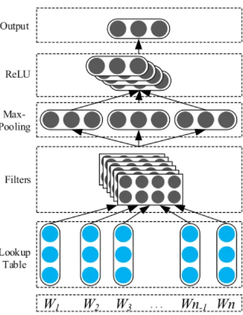
We transform each input text into the concatenation of all word vectors, each of which is a word embedding that captures the syntactic and semantic meanings of the word. In this way, we can represent the input text as a vector sequence = , , … , . The vector sequence can be converted into a matrix ∈ × , where is the dimension of the word embedding and is the length of the text. After encoding the input text, we use a convolutional layer to extract the local features, then apply max-pooling and a non-linear layer to merge all local features into a global representation. Lookup Table Filters ReLU Output Max-Pooling W1 W2 W3 · · · Wn-1 Wn
Figure 1. Convolutional neural network with multiple convolutional filters for n-gram feature extraction.
Specifically, the convolutional layer extracts local features by sliding continuously window shaped filters with full rows of the matrix T. The width of the filters is the same as width d of the word embedding. The height ℎ of filters is a number of adjacent rows. Empirical research demonstrates that sliding filters over 2–5 words at a time could achieve strong performance [31]. The filters slide over matrix A and perform convolutional operations. Let : denote sub-matrix of T from row to row ; denotes the th filter. Formally, the output of the convolutional layer for -th filter is computed as:
[
]
T : 1 i i o = i i h+ − ⊗w (1)(
)
i ic
=
f o b
+
(2)where ⊗ is element-wise multiplication, is the feature learned by the -th filter, is the bias, and is the activation function that can be sigmoid, tangent, etc. In our case, we chose Rectified
Figure 1. Convolutional neural network with multiple convolutional filters for n-gram feature extraction.
We transform each input text into the concatenation of all word vectors, each of which is a word embedding that captures the syntactic and semantic meanings of the word. In this way, we can represent the input text as a vector sequenceV = {v1,v2, . . . ,vn}. The vector sequence Vcan be converted into a matrixT∈Rs×d, wheredis the dimension of the word embedding andsis the length of the text. After encoding the input text, we use a convolutional layer to extract the local features, then apply max-pooling and a non-linear layer to merge all local features into a global representation. Specifically, the convolutional layer extracts local features by sliding continuously window shaped filters with full rows of the matrixT. The widthlof the filters is the same as widthdof the word embedding. The heighthof filters is a number of adjacent rows. Empirical research demonstrates that sliding filters over 2–5 words at a time could achieve strong performance [31]. The filters slide over matrixAand perform convolutional operations. LetT[i:j]denote sub-matrix ofTfrom rowito rowj; widenotes thei-th filter. Formally, the output of the convolutional layer fori-th filter is computed as:
oi=T[i:i+h−1]⊗wi (1)
ci = f(oi+b) (2)
where⊗is element-wise multiplication,ci is the feature learned by thei-th filter,bis the bias, and f is the activation function that can be sigmoid, tangent, etc. In our case, we chose Rectified Linear
Sustainability2018,10, 219 6 of 22
Unit ReLU as the nonlinear activation function. After that, we combine all local features map c via a max-pooling function. The max-pooling function applies to each feature mapcito reduce the dimensionality and capture the highest value from the features. Fornfilters, the generatednfeature maps can be treated as the input of BiLSTM,
W ={c1,c2, . . . ,cn} (3)
Here, comma represents column vector concatenation andciis the feature map generated with thei-th filter.
3.2. Long Dependency Feature Extraction Based on Bidirectional LSTM
The LSTM has a series of repeating modules of a neural network for each time step as in standard RNN. At each time step, the cell statect(old hidden stateht−1, the input at the current time stepxt) is controlled by a set of gates, the forget gate ft, the input gateit, and the output gateot. These gates using previous hidden stateht−1and current inputxito jointly make decide how to update the current memory cellctand the current hidden stateht. The LSTM transition functions are defined as follows:
Input gates: it=σg(Wi⊗[ht−1,xt] +bi) (4) Forget gates: ft=σg Wf⊗[ht−1,xt] +bf (5) tput gates: ot=σc(Wo⊗[ht−1,xt] +bo) (6) Cell states: ct= ft ⊗ct−1+it⊗qt (7) Cell outputs: ht=ot⊗σc(ct) (8)
Here,σgis the logistic sigmoid function f(x) = 1+1e−x, that has an output in [0, 1],σcdenotes a
hyperbolic tangent function, and⊗denotes the element-wise multiplication.
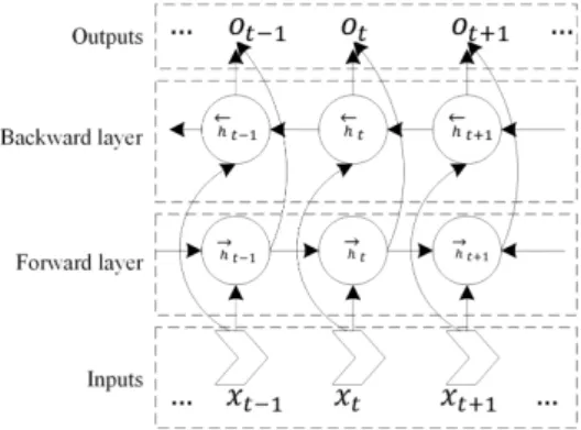
The LSTM is designed for learning long-term dependencies of time-series data, and it is especially true in the case of bidirectional long–short-term memory networks (BiLSTM), since BiLSTM enables us to classify each element in a sequence while using information from that element’s past and future. Figure2shows the architecture of BiLSTM. Therefore, we choose BiLSTM to stack to the convolution layer to learn such dependencies in the sequence of higher-level features.
Linear Unit ReLU as the nonlinear activation function. After that, we combine all local features map via a max-pooling function. The max-pooling function applies to each feature map to reduce the dimensionality and capture the highest value from the features. For n filters, the generated n feature maps can be treated as the input of BiLSTM,
{
1,
2, ,
n}
W
=
c c
…
c
(3)Here, comma represents column vector concatenation and is the feature map generated with the -th filter.
3.2. Long Dependency Feature Extraction Based on Bidirectional LSTM
The LSTM has a series of repeating modules of a neural network for each time step as in standard RNN. At each time step, the cell state (old hidden state ℎ , the input at the current time step ) is controlled by a set of gates, the forget gate , the input gate , and the output gate . These gates using previous hidden state ℎ and current input to jointly make decide how to update the current memory cell and the current hidden state ℎ . The LSTM transition functions are defined as follows: Input gates:
[
]
(
1)
σ
,
t g i t t ii
=
W
⊗
h
−x
+
b
(4) Forget gates:[
]
(
1)
σ , t g f t t f f = W ⊗ h− x +b (5) Output gates:[
]
(
1)
σ , t c o t t o o = W ⊗ h− x +b (6) Cell states: 1 t t t t tc
= ⊗
f
c
−+ ⊗
i
q
(7) Cell outputs:σ
( )
t t c th
= ⊗
o
c
(8)Here, is the logistic sigmoid function ( ) 1
1 x
f x e−
=
+ , that has an output in [0, 1], denotes a hyperbolic tangent function, and ⊗ denotes the element-wise multiplication.
The LSTM is designed for learning long-term dependencies of time-series data, and it is especially true in the case of bidirectional long–short-term memory networks (BiLSTM), since BiLSTM enables us to classify each element in a sequence while using information from that element’s past and future. Figure 2 shows the architecture of BiLSTM. Therefore, we choose BiLSTM to stack to the convolution layer to learn such dependencies in the sequence of higher-level features.
Figure 2. The architecture of BiLSTM. Figure 2.The architecture of HFEM.
3.3. The Architecture of the Hierarchical Feature Extraction Model and Algorithm
Based on the analyses above, a hybrid neural network model based on convolutional and long short-term memory neural networks, is proposed. The architecture of hierarchical feature extraction model (HFEM) is shown in Figure3, and the algorithm can be detailed as follows:
Input: Narrative text in patent documents.
Output: Probabilities of IPC labels for each patent document.
(1) Split the document into four sections, keep the top 150 words of each section.
(2) Initialize the text with pertained word embedding by looking up the word embedding lookup table, then each patent document is represented by four matrices with dimension 150×100. (3) The four matrices are fed in to four independent CNN channels, each channel applies 128 filters
with the dimensions of 3×100. The convolutional operation converts four input channels into four feature maps with the dimension of 148×128.
(4) Concatenation, maximum, average, and summation strategies are employed to join the feature maps. After four concatenation operations, four kinds of feature maps are obtained with the dimension of 592×128, 148×128, 148×128, and 148×128 respectively.
(5) The four feature maps are fed into four BiLSTM networks with 128 forward and backward LSTM neurons. After the BiLSTM network, each feature map is reduced to a matrix of 1×256. (6) Sigmoid function is utilized to calculate the feature vector’s probabilities for each label.
Sustainability 2018, 10, 219 7 of 22
3.3. The Architecture of the Hierarchical Feature Extraction Model and Algorithm
Based on the analyses above, a hybrid neural network model based on convolutional and long short-term memory neural networks, is proposed. The architecture of hierarchical feature extraction model (HFEM) is shown in Figure 3, and the algorithm can be detailed as follows:
Input: Narrative text in patent documents.
Output: Probabilities of IPC labels for each patent document.
(1) Split the document into four sections, keep the top 150 words of each section.
(2) Initialize the text with pertained word embedding by looking up the word embedding lookup table, then each patent document is represented by four matrices with dimension 150 × 100. (3) The four matrices are fed in to four independent CNN channels, each channel applies 128 filters
with the dimensions of 3 × 100. The convolutional operation converts four input channels into four feature maps with the dimension of 148 × 128.
(4) Concatenation, maximum, average, and summation strategies are employed to join the feature maps. After four concatenation operations, four kinds of feature maps are obtained with the dimension of 592 × 128, 148 × 128, 148 × 128, and 148 × 128 respectively.
(5) The four feature maps are fed into four BiLSTM networks with 128 forward and backward LSTM neurons. After the BiLSTM network, each feature map is reduced to a matrix of 1 × 256.
(6) Sigmoid function is utilized to calculate the feature vector’s probabilities for each label.
Figure 3. The architecture of HFEM.
Since each patent document consists of multiple narrative text sections, the classification model should take various sections into account. We apply a CNN to extract n-gram features from mechanical patent documents with consecutive window filters. After that, we combine all the local n-gram feature maps extracted from different sections, via four kinds of concatenation strategies to concatenate local features into global ones. Especially, we did not employ a max-pooling layer to the convolutional network due to the fact that a max-pooling operation will break the continuous sequence organization of selected features. However, the BiLSTM is explicitly designed for sequence data. We do not apply pooling after the convolution operations since we stack the BiLSTM on top of the CNN.
After the CNN layer, the four channel inputs have been converted into four feature maps. We use , , and to denote the feature maps from the four input channels, respectively. Then we employ concatenation, maximum, average and summation strategies to concatenate features into global ones.
CON title abstract claims description
W =W ⊕W ⊕W ⊕W (9)
Here, ⊕ denotes the matrix concatenation operation and denotes the result after concatenation operation, so the shape of the matrix will be four times that of the feature map.
( , , , )
MAX title abstract claims description
W =MAX W W W W (10)
Figure 3.The architecture of HFEM.
Since each patent document consists of multiple narrative text sections, the classification model should take various sections into account. We apply a CNN to extractn-gram features from mechanical patent documents with consecutive window filters. After that, we combine all the localn-gram feature maps extracted from different sections, via four kinds of concatenation strategies to concatenate local features into global ones. Especially, we did not employ a max-pooling layer to the convolutional network due to the fact that a max-pooling operation will break the continuous sequence organization of selected features. However, the BiLSTM is explicitly designed for sequence data. We do not apply pooling after the convolution operations since we stack the BiLSTM on top of the CNN.
After the CNN layer, the four channel inputs have been converted into four feature maps. We use Wtitle, Wabstract, Wclaims and Wdescription to denote the feature maps from the four input channels, respectively. Then we employ concatenation, maximum, average and summation strategies to concatenate features into global ones.
Here, ⊕ denotes the matrix concatenation operation and WCON denotes the result after concatenation operation, so the shape of theWCONmatrix will be four times that of the feature map.
WMAX = MAX(Wtitle,Wabstract,Wclaims,Wdescription) (10) where theMAX()operation selects the maximum value from each feature map.
WAVE=AVE(Wtitle,Wabstract,Wclaims,Wdescription) (11) where theAVE()conducts the sum operation of each feature map first, then averages the value.
WSU M=Wtitle+Wabstract+Wclaims+Wdescription (12) Here,+denotes the summation operation andWSU Mdenotes the sum of each feature map. Then, theWCON, WMAX,WAVEandWSU Mchannel features are fed into the BiLSTM jointly. Our approach is different from those methods that use multi-layer CNNs and train the CNN and LSTM separately. We treat the model as an entire network and train the CNN and BiLSTM layers simultaneously. We adopt Adaptive Moment Estimation (ADAM) [32] to minimize the objective function to solve the optimization problem. For the training procedure, we randomly feed the model with a batch of training set until the results converge.
4. Datasets and Evaluation Metrics
In order to check the performance of the proposed algorithm, we established the training, validation and test datasets, all of which are subsets of the CLEF-IP 2011 dataset [33]. The CLEF-IP 2011 dataset consists of more than 2.6 million patent documents from the European Patent Office (EPO) and 400,000 patent documents from the World Intellectual Property Organization (WIPO), representing of 1.35 million (each patent may consist of multiple patent documents) patents filed between 1978 and 2009. These 1.35 million patents contain three kinds olanguage contents, namely English, German, and French.
Generally speaking, a patent document includes bibliographic information, a title, document number, issued date, patent type, classification information, a list of inventors, a list of applicant companies or individuals, abstract, claims section, and a full-text description. More specifically, the title of a patent indicates the name of the patent; the abstract part gives a brief technical description of the innovation; the patent type explains the patent type, and the classification part presents one or multiple class labels. The claim section’s main function is to protect the inventors’ rights. The description section describes the process, the machine, manufacture, composition of matter, or improvement invented, a brief summary and the background of the invention, the detailed description, and a brief description of its application. The documents also contain meta-information on the assignee, date of application, inventor, etc.
In our experiments, we extracted records from the CLEF-IP 2011 dataset that contain at least one IPC-R classification label, which belongs to section F and the title, abstract, claims, and description textual content in English, namely M-CLEF. Figure4shows the yearly distribution of the patent document quantities in the M-CLEF dataset. In the IPC hierarchic taxonomy, section F includes patent applications ranging from the mechanical engineering, lighting, heating and weapons fields. All different document versions for a single patent are merged into a single document with fields updated from its latest versions. After data cleaning, the final M-CLEF dataset consists of 107,302 patent documents. In order to approach a realistic patent classification scenario, we split the dataset into training, validation, and test datasets based on time, so that patents in the training and validation datasets have timestamps earlier than those in the test datasets. More specifically, we used the patents published during 2006 to 2008 as test data and randomly split the rest of patents (all before 2006) into 80% and 20%, as training and validation datasets, respectively. Table1shows the detailed numbers
for each dataset used in our experiments. We conduct a series of experiments on the multi-label patent classification task. On average, each patent in the training set has 1.4 classification labels at the
subclass level.Sustainability 2018, 10, 219 9 of 22
Figure 4. The distribution of the dataset.
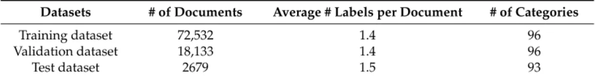
Table 1. Brief information of the training, validation and test datasets.
Datasets # of Documents Average # Labels per Document # of Categories
Training dataset 72,532 1.4 96
Validation dataset 18,133 1.4 96
Test dataset 2679 1.5 93
The M-CLEF dataset consists of the four sections of subset title, abstract, claims, and description. In previous studies, researchers found that methods based on only patent title and abstract score lower than those based on the full content of patent documents [34]. Therefore, we used the entire document content as different input channels for our models to determine the effect of various sections in the patent content on the classification performance.
Figure 5 shows the detailed text preprocessing procedure and research framework. First of all, we selected the patents from the CLEF-IP 2011 dataset, which are filled in English and belong to section F. Then, we conducted the followings text preprocessing procedures on the selected patent texts (M-CLEF): (1) Remove all punctuation and convert to lowercase; (2) Replace all contiguous whitespace sequences with a single space; (3) Separate unrelated blocks of text with a newline character. After these text preprocessing procedures, the CLEF dataset was converted to the M-CLEF corpus. Then the corpus was fed to the CBOW model to train word embeddings. The remaining descriptions of Figure 5 are presented above.
For each experiment, we used the followings evaluation metrics to evaluate various methods, since we conducted multi-label patent classification experiments. Firstly, we predicted one, five and 10 IPC labels for each patent document respectively. Then we calculated
, , and 1 for each prediction.
Figure 4.The distribution of the dataset.
Table 1.Brief information of the training, validation and test datasets.
Datasets # of Documents Average # Labels per Document # of Categories
Training dataset 72,532 1.4 96
Validation dataset 18,133 1.4 96
Test dataset 2679 1.5 93
The M-CLEF dataset consists of the four sections of subset title, abstract, claims, and description. In previous studies, researchers found that methods based on only patent title and abstract score lower than those based on the full content of patent documents [34]. Therefore, we used the entire document content as different input channels for our models to determine the effect of various sections in the patent content on the classification performance.
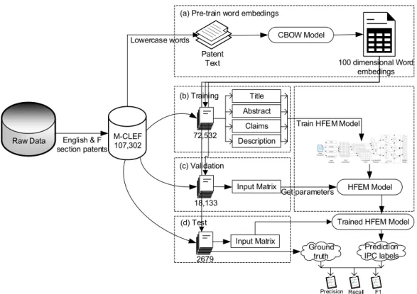
Figure5shows the detailed text preprocessing procedure and research framework. First of all, we selected the patents from the CLEF-IP 2011 dataset, which are filled in English and belong to section F. Then, we conducted the followings text preprocessing procedures on the selected patent texts (M-CLEF): (1) Remove all punctuation and convert to lowercase; (2) Replace all contiguous whitespace sequences with a single space; (3) Separate unrelated blocks of text with a newline character. After these text preprocessing procedures, the M-CLEF dataset was converted to the M-CLEF corpus. Then the corpus was fed to the CBOW model to train word embeddings. The remaining descriptions of Figure5are presented above.
For each experiment, we used the followings evaluation metrics to evaluate various methods, since we conducted multi-label patent classification experiments. Firstly, we predicted one, five and 10 IPC labels for each patent document respectively. Then we calculatedPrecisonweighted,Recallweighted, andF1weightedfor each prediction.
Sustainability 2018, 10, 219 10 of 22
Raw Data English & F M-CLEF107,302 section patents
Patent Text Lowercase words
(a) Pre-train word embedings
CBOW Model 100 dimensional Word embedings Title Abstract Claims (b) Training Description
Train HFEM Model
(c) Validation (d) Test 72,532 18,133 2679 Input Matrix Input Matrix HFEM Model Get parameters Prediction IPC labels Precision F1 Ground truth Recall
Trained HFEM Model
Figure 5. Data preprocessing and data flow diagram.
For each patent document, the number of outcome labels of our approach (prediction labels) that matched the available IPC labels (available labels), without taking the exact order into account, are considered to be true positives (TP). False positives (FP) are the labels predicted by our approach that do not match the available IPC labels. As false negatives (FN), we considered the labels that should have been predicted by our approach, but were not. True negatives (TN) are the labels that, correctly, were not predicted by our approach. Then the precision and recall could be calculated as follows:
|available labels
prediction labels|
=
|prediction labels|
scorePrecison
∩
(13)|available labels
prediction labels|
=
|available labels|
scoreRecall
∩
(14)After calculating each and for each patent, then the weighted
average , and 1 can be calculated as follows:
1
1
=
Total Samples weighted i iPrecison
Precison
Total Samples
= (15) 11
Total Samp weig le ht s ed i iRecall
Recall
Total Samples
==
(16)1
2
weighted weighted weighted weighted weightedPrecison
Recall
F
Precison
Recall
×
+
×
=
(17)The , and 1 are denoted as , , and 1
respectively. We use # to denote the number of topmost labels returned by the model, and then we can denote the measures as @#, @#, and 1@# respectively.
Figure 5.Data preprocessing and data flow diagram.
For each patent document, the number of outcome labels of our approach (prediction labels) that matched the available IPC labels (available labels), without taking the exact order into account, are considered to be true positives (TP). False positives (FP) are the labels predicted by our approach that do not match the available IPC labels. As false negatives (FN), we considered the labels that should have been predicted by our approach, but were not. True negatives (TN) are the labels that, correctly, were not predicted by our approach. Then the precision and recall could be calculated as follows:
Precisonscore= |available labels∩prediction labels|
|prediction labels| (13)
Recallscore= |available labels∩prediction labels|
|available labels| (14)
After calculating eachPrecisonscore andRecallscorefor each patent, then the weighted average Precisonweighted,RecallweightedandF1weightedcan be calculated as follows:
Precisonweighted = 1 Total Samples Total Samples
∑
i=1 Precisoni (15) Recallweighted = 1 Total Samples Total Samples∑
i=1 Recalli (16) F1weighted=2×Precisonweighted×Recallweighted Precisonweighted+Recallweighted
(17) ThePrecisonweighted,RecallweightedandF1weightedare denoted asP,R, andF1 respectively. We use # to denote the number of topmost labels returned by the model, and then we can denote the measures asP@#,R@#, andF1@# respectively.
5. Performance Analysis of HFEM with Different Concatenation Strategies
Since the concatenation strategies influence the performance of our algorithm, we implemented the HFEM with different concatenation strategies using Keras [35], a Python deep learning library, which supports efficient symlic dntiation and transparent use of a Graphics Processing Unit (GPU). To benefit from the efficiency of parallel computation of the tensor, we trained the model on a GPU.
First, since the convolutional layers in our model demand fixed-length inputs, we used MAX_LENto denote the maximum length of text for each input section in the training and test dataset. We employed the CBOW algorithm [36] to pre-train our M-CLEF corpora into word embeddings, with a dimensionality of 100, 200, and 300.
We initialized each section text that had a length less than MAX_LEN with a (MAXLEN−CURLEN)×d zero vector at the end of the representation matrix. Nevertheless, for the texts which had a length longer thanMAX_LEN, we simply cut extra words at the end of these texts to reachMAX_LEN. Therefore, all text was converted to representation matrixes of the same shape. The shape of the final matrices isMAX_LEN×d. For the classification labels, the whole number of categories in the M-CLEF dataset was 96. Each patent had at least one classification label. In the case of multi-label classification task, we represented the joint set of labels with a binary indicator matrix. For example, given several patents with labels as follows—p1={F03G},p2={F16B,F16L}, p3={F16B}—the label set should beS={F03G,F16B,F16L}. Each patent could be represented as one row of the label matrix with binary values; the label matrix
1 0 0 0 1 1 0 1 0 represents labelF03G
in the first patent, labels F16BandF16Lin the second patent and labels F16B in the third patent. The non-zero elements correspond to the subset of labels.
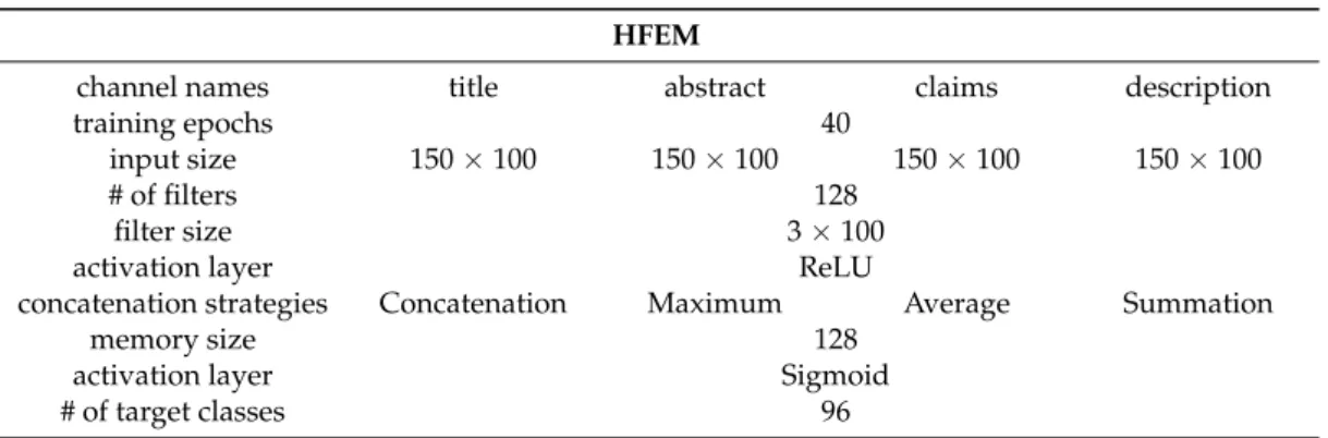
In order to determine which concatenation strategy offered the best effect, we implemented four versions of HFEM with different concatenation strategies. The detailed configuration parameters are listed in Table2. Each variant of HFEM takes four input channels and each channel uses 150 word vectors to concatenate into a text matrix of 150×100. A total of 128 convolutional filters with size of 3×100 were applied in the convolutional layer and a ReLU function was subsequently used as the non-linear activation function. Then the concatenation strategy was employed to concatenate the extracted feature maps. The jointed feature maps were fed to BiLSTM, consisting of 128 forward and backward LSTM neurons. Finally, a fully-connected layer with sigmoid activation was used to calculate the probabilities of 96 IPC labels.
Table 2.The parameters of the HFEM model. HFEM
channel names title abstract claims description
training epochs 40
input size 150×100 150×100 150×100 150×100
# of filters 128
filter size 3×100
activation layer ReLU
concatenation strategies Concatenation Maximum Average Summation
memory size 128
activation layer Sigmoid
# of target classes 96
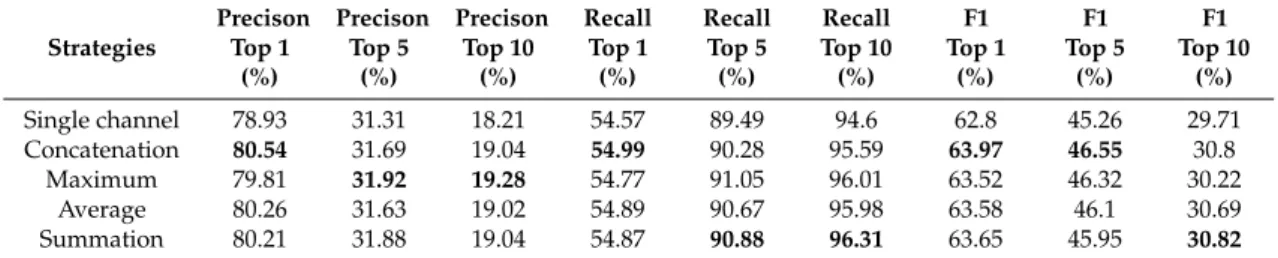
Five experiments were conducted to determine which concatenation strategy can provide the best performance, and the statistical results are shown in Table3. As we can summarize from Table3, the single channel HFEM achieved decent results, taking the entire text as the single channel input. At the same time, all the other four multi-channel variants of HFEM improved the performance in nine evaluation metrics. In the scenario of predicting one IPC label for each patent, the concatenation
scheme obtained the best performance for three evaluating criteria, namely improving the precision, recall and F1 scores by 1.61%, 0.42% and 1.17%, respectively, compared with the single channel HFEM. The maximum scheme had a slight advantage in predicting five IPC labels for each patent, and achieved the best performance for two out of three criteria. Regarding the prediction of 10 IPC labels, the best performance was achieved by different concatenation schemes. Nevertheless, we found that the concatenation scheme obtained the best performance in five out of nine evaluation metrics. Hence, we choose the HFEM with concatenation scheme as our ultimate version model for all experiments.
Table 3.Performance of HFEM with different strategies using the narrative text as input.
Strategies Precison Top 1 (%) Precison Top 5 (%) Precison Top 10 (%) Recall Top 1 (%) Recall Top 5 (%) Recall Top 10 (%) F1 Top 1 (%) F1 Top 5 (%) F1 Top 10 (%) Single channel 78.93 31.31 18.21 54.57 89.49 94.6 62.8 45.26 29.71 Concatenation 80.54 31.69 19.04 54.99 90.28 95.59 63.97 46.55 30.8 Maximum 79.81 31.92 19.28 54.77 91.05 96.01 63.52 46.32 30.22 Average 80.26 31.63 19.02 54.89 90.67 95.98 63.58 46.1 30.69 Summation 80.21 31.88 19.04 54.87 90.88 96.31 63.65 45.95 30.82
6. Comparison and Analysis with Other Methods
In this section, we first describe the implementation of three baseline models for the classification task, consisting of CNN, LSTM, and BiLSTM, then give a detailed description of how to conduct the experiments. Five groups of experiments are carried out to validate the feasibility and effectiveness of our HEFM model, and then the results and related analyses are presented.
6.1. Experimental Setup
We compare the HFEM with the following baseline neural network models for mechanical patent classification.
1. CBOW+CNN: We converted patent text using word embeddings pre-trained with the CBOW algorithm into the input matrix and then trained a CNN model with 128 filters for classifying mechanical patent documents.
2. CBOW+LSTM: We converted patent text using word embeddings pre-trained with the CBOW algorithm into the input matrix and then trained an LSTM model with 128 memory LSTM units for classifying mechanical patent documents.
3. CBOW+BiLSTM: We converted patent text using word embeddings pre-trained with the CBOW algorithm into the input matrix and trained a BiLSTM model with 128 forward and backward LSTM units for classifying mechanical patent documents.
The detailed hyper-parameters are listed in Table4. For each baseline method, the training epoch was fixed to 40, and the number of input words was set to 150 when only taking one section from the entire patent document. The number was set to 600 when the entire text was used by the model, and finally, a fully-connected layer with sigmoid activation function was connected to 96 categories from the IPC label matrix.
Table 4.Hyper-parameters for baseline methods.
Hyper-Parameters CNN LSTM BiLSTM training epochs 40 40 40 input size 600×100 600×100 600×100 # of filters 128 - -memory size - 128 128 max-pooling size 2 - -# of target classes 96 96 96
6.2. Experimental Results and Discussion
We conducted a series of experiments on our HFEM and the baseline models, using the entire narrative text from the M-CLEF dataset. The results are shown in Figures6–11and Tables5and6.
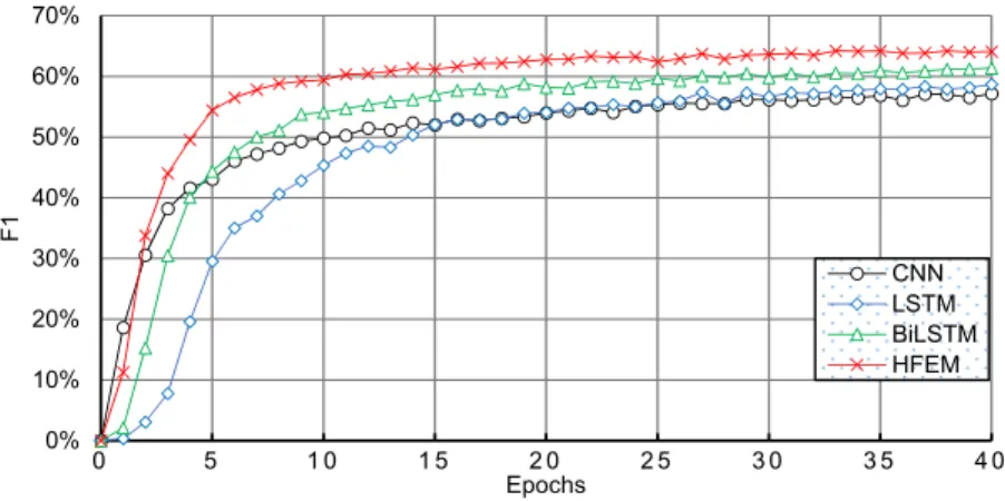
According to Figure6, it can be seen that HFEM obtained approximate precision, recall, and F1 scores of 81%, 55%, and 64%, respectively, while the best performance of the three baseline models was 78%, 52%, and 64%.This indicates that HFEM improved the performance by 3% in terms of the three evaluation criteria. Figure6a illustrated the precision scores achieved by four models. HFEM showed its overwhelming advantage in precision when compared with the three baseline methods. Besides, HFEM also demonstrated its superiority in recall, as shown in Figure6b. From the evaluation criterion of F1, the four approaches show very similar performance in terms of precision and recall, and the results are displayed in Figure6c. Furthermore, as we can see from Figure6, the HFEM model converged faster than the three baseline models. The precision, recall, and F1 scores for HFEM tended to converge before 15 epochs, while the other models needed at least 20 epochs to reach steady state. In addition, we report the performance of these four models for nine evaluation indictors in Table5. HFEM obtained the best performance in predicting one label for each patent document as well as in predicting five and ten labels. The experimental results demonstrate and verify the feasibility and effectiveness of our HFEM model for mechanical patent classification.
Moreover, we were interested in understanding which section in the patent document has more representative features for classification. We conducted a series of orthogonal experiments by separately using four sections as input and four models as classifiers. More specifically, we used the title, abstract, claims and description separately as input for the CNN, LSTM, BiLSTM, and HFEM models.
Sustainability 2018, 10, 219 13 of 22
6.2. Experimental Results and Discussion
We conducted a series of experiments on our HFEM and the baseline models, using the entire narrative text from the M-CLEF dataset. The results are shown in Figures 6–11 and Tables 5 and 6.
According to Figure 6, it can be seen that HFEM obtained approximate precision, recall, and F1 scores of 81%, 55%, and 64%, respectively, while the best performance of the three baseline models was 78%, 52%, and 64%.This indicates that HFEM improved the performance by 3% in terms of the three evaluation criteria. Figure 6a illustrated the precision scores achieved by four models. HFEM showed its overwhelming advantage in precision when compared with the three baseline methods. Besides, HFEM also demonstrated its superiority in recall, as shown in Figure 6b. From the evaluation criterion of F1, the four approaches show very similar performance in terms of precision and recall, and the results are displayed in Figure 6c. Furthermore, as we can see from Figure 6, the HFEM model converged faster than the three baseline models. The precision, recall, and F1 scores for HFEM tended to converge before 15 epochs, while the other models needed at least 20 epochs to reach steady state. In addition, we report the performance of these four models for nine evaluation indictors in Table 5. HFEM obtained the best performance in predicting one label for each patent document as well as in predicting five and ten labels. The experimental results demonstrate and verify the feasibility and effectiveness of our HFEM model for mechanical patent classification.
Moreover, we were interested in understanding which section in the patent document has more representative features for classification. We conducted a series of orthogonal experiments by separately using four sections as input and four models as classifiers. More specifically, we used the title, abstract, claims and description separately as input for the CNN, LSTM, BiLSTM, and HFEM models.
(a) Precision scores of four models using the entire text as input.
(b) Recall scores of four models using the entire text as input.
0% 10% 20% 30% 40% 50% 60% 70% 80% 90% 0 5 1 0 1 5 2 0 2 5 3 0 3 5 4 0 Pr ecision Epochs CNN LSTM BiLSTM HFEM 0% 10% 20% 30% 40% 50% 60% 0 5 1 0 1 5 2 0 2 5 3 0 3 5 4 0 Recall Epochs CNN LSTM BiLSTM HFEM Figure 6.Cont.
Sustainability 2018, 10, 219 14 of 22
(c) F1 scores of four models using the entire text as input.
Figure 6. Performance using the entire text as input.
Table 5. Results of various models using the narrative text as input.
Algorithms P@1% P@5% P@10 % R@1 % R@5 % R@10 % F1@1 % F1@5 % F1@10 % CNN 71.34 29.89 17.43 50.08 86.81 92.93 57.02 43.09 28.35 LSTM 74.44 30.53 18.44 51.96 86.14 92.96 59.26 43.72 29.73 BiLSTM 77.71 30.96 18.83 53.57 88.1 94.67 61.55 44.53 30.24 HFEM 80.54 31.69 19.04 54.99 90.28 95.59 63.97 46.55 30.8
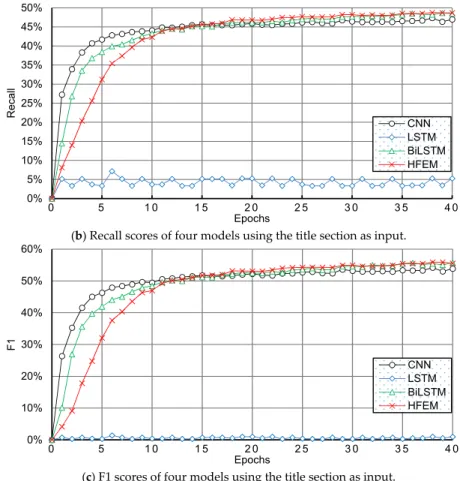
First of all, we used the title section as the input for the models. Figure 7 illustrates the performance of the four models on the title section. From the figure, we can find that the LSTM model achieved quite poor performance whether in terms of precision (see Figure 7a), recall (see Figure 7b), or F1 score (see Figure 7c). The CNN and BiLSTM models obtained decent results, while the convergence of CNN was faster than the other models. Although the convergence of our HFEM model was not as fast as CNN, after 10 epochs, it began to achieve comparable results. After 20 epochs, our model began to outperform the other methods. The best precision of our model was around 72%, while it was only 5% for LSTM. We inspected the M-CLEF dataset and found the title section in the patent documents to be quite short. On average, there are less than ten words in the title section, which explains why the LSTM model achieved poor performance.
(a) Precision scores of four models using the title section as input.
0% 10% 20% 30% 40% 50% 60% 70% 0 5 1 0 1 5 2 0 2 5 3 0 3 5 4 0 F1 Epochs CNN LSTM BiLSTM HFEM 0% 10% 20% 30% 40% 50% 60% 70% 80% 0 5 1 0 1 5 2 0 2 5 3 0 3 5 4 0 Pr ecision Epochs CNN LSTM BiLSTM HFEM
Figure 6.Performance using the entire text as input. Table 5.Results of various models using the narrative text as input.
Algorithms P@1% P@5% P@10% R@1% R@5% R@10% F1@1% F1@5% F1@10% CNN 71.34 29.89 17.43 50.08 86.81 92.93 57.02 43.09 28.35 LSTM 74.44 30.53 18.44 51.96 86.14 92.96 59.26 43.72 29.73 BiLSTM 77.71 30.96 18.83 53.57 88.1 94.67 61.55 44.53 30.24 HFEM 80.54 31.69 19.04 54.99 90.28 95.59 63.97 46.55 30.8
First of all, we used the title section as the input for the models. Figure7illustrates the performance of the four models on the title section. From the figure, we can find that the LSTM model achieved quite poor performance whether in terms of precision (see Figure7a), recall (see Figure7b), or F1 score (see Figure7c). The CNN and BiLSTM models obtained decent results, while the convergence of CNN was faster than the other models. Although the convergence of our HFEM model was not as fast as CNN, after 10 epochs, it began to achieve comparable results. After 20 epochs, our model began to outperform the other methods. The best precision of our model was around 72%, while it was only 5% for LSTM. We inspected the M-CLEF dataset and found the title section in the patent documents to be quite short. On average, there are less than ten words in the title section, which explains why the LSTM model achieved poor performance.
Sustainability 2018, 10, 219 14 of 22
(c) F1 scores of four models using the entire text as input.
Figure 6. Performance using the entire text as input.
Table 5. Results of various models using the narrative text as input.
Algorithms P@1% P@5% P@10 % R@1 % R@5 % R@10 % F1@1 % F1@5 % F1@10 % CNN 71.34 29.89 17.43 50.08 86.81 92.93 57.02 43.09 28.35 LSTM 74.44 30.53 18.44 51.96 86.14 92.96 59.26 43.72 29.73 BiLSTM 77.71 30.96 18.83 53.57 88.1 94.67 61.55 44.53 30.24 HFEM 80.54 31.69 19.04 54.99 90.28 95.59 63.97 46.55 30.8
First of all, we used the title section as the input for the models. Figure 7 illustrates the performance of the four models on the title section. From the figure, we can find that the LSTM model achieved quite poor performance whether in terms of precision (see Figure 7a), recall (see Figure 7b), or F1 score (see Figure 7c). The CNN and BiLSTM models obtained decent results, while the convergence of CNN was faster than the other models. Although the convergence of our HFEM model was not as fast as CNN, after 10 epochs, it began to achieve comparable results. After 20 epochs, our model began to outperform the other methods. The best precision of our model was around 72%, while it was only 5% for LSTM. We inspected the M-CLEF dataset and found the title section in the patent documents to be quite short. On average, there are less than ten words in the title section, which explains why the LSTM model achieved poor performance.
(a) Precision scores of four models using the title section as input.
0% 10% 20% 30% 40% 50% 60% 70% 0 5 1 0 1 5 2 0 2 5 3 0 3 5 4 0 F1 Epochs CNN LSTM BiLSTM HFEM 0% 10% 20% 30% 40% 50% 60% 70% 80% 0 5 1 0 1 5 2 0 2 5 3 0 3 5 4 0 Pr ecision Epochs CNN LSTM BiLSTM HFEM Figure 7.Cont.
Sustainability 2018, 10, 219 15 of 22
(b) Recall scores of four models using the title section as input.
(c) F1 scores of four models using the title section as input.
Figure 7. Performance of four models on the title section.
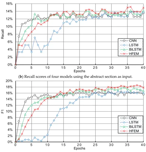
Then, we conducted experiments using the abstract section. Figure 8 shows the performance of the four models on the abstract section. As illustrated in Figure 8a below, the best performance for precision achieved by each model was 60.4%, 63.1%, 67.2%, and 70.3%. At the very beginning, the BiLSTM and CNN models performed better in recall than HFEM, but the HFEM model obtained better recall scores than the others after 15 epochs (see Figure 8b). Furthermore, we found that the curves of Figure 8c are not as smooth as in Figure 7c. After inspecting the M-CLEF dataset, we found that some documents have a missing abstract section, which may have led to the unsmooth curve phenomenon.
(a) Precision scores of four models using the abstract section as input.
0% 5% 10% 15% 20% 25% 30% 35% 40% 45% 50% 0 5 1 0 1 5 2 0 2 5 3 0 3 5 4 0 Recall Epochs CNN LSTM BiLSTM HFEM 0% 10% 20% 30% 40% 50% 60% 0 5 1 0 1 5 2 0 2 5 3 0 3 5 4 0 F1 Epochs CNN LSTM BiLSTM HFEM 0% 10% 20% 30% 40% 50% 60% 70% 0 5 1 0 1 5 2 0 2 5 3 0 3 5 4 0 Pr ecision Epochs CNN LSTM BiLSTM HFEM
Figure 7.Performance of four models on the title section.
Then, we conducted experiments using the abstract section. Figure8shows the performance of the four models on the abstract section. As illustrated in Figure8a below, the best performance for precision achieved by each model was 60.4%, 63.1%, 67.2%, and 70.3%. At the very beginning, the BiLSTM and CNN models performed better in recall than HFEM, but the HFEM model obtained better recall scores than the others after 15 epochs (see Figure8b). Furthermore, we found that the curves of Figure8c are not as smooth as in Figure7c. After inspecting the M-CLEF dataset, we found that some documents have a missing abstract section, which may have led to the unsmooth curve phenomenon.
(b) Recall scores of four models using the title section as input.
(c) F1 scores of four models using the title section as input.
Figure 7. Performance of four models on the title section.
Then, we conducted experiments using the abstract section. Figure 8 shows the performance of the four models on the abstract section. As illustrated in Figure 8a below, the best performance for precision achieved by each model was 60.4%, 63.1%, 67.2%, and 70.3%. At the very beginning, the BiLSTM and CNN models performed better in recall than HFEM, but the HFEM model obtained better recall scores than the others after 15 epochs (see Figure 8b). Furthermore, we found that the curves of Figure 8c are not as smooth as in Figure 7c. After inspecting the M-CLEF dataset, we found that some documents have a missing abstract section, which may have led to the unsmooth curve phenomenon.
(a) Precision scores of four models using the abstract section as input. 0% 5% 10% 15% 20% 25% 30% 35% 40% 45% 50% 0 5 1 0 1 5 2 0 2 5 3 0 3 5 4 0 Recall Epochs CNN LSTM BiLSTM HFEM 0% 10% 20% 30% 40% 50% 60% 0 5 1 0 1 5 2 0 2 5 3 0 3 5 4 0 F1 Epochs CNN LSTM BiLSTM HFEM 0% 10% 20% 30% 40% 50% 60% 70% 0 5 1 0 1 5 2 0 2 5 3 0 3 5 4 0 Pr ecision Epochs CNN LSTM BiLSTM HFEM Figure 8.Cont.
Sustainability 2018, 10, 219 16 of 22
(b) Recall scores of four models using the abstract section as input.
(c) F1 scores of four models using the abstract section as input.
Figure 8. Performance of four models using the abstract section as input.
After that, the claims section was used in the following experiments. Figure 9 illustrates the performance of the four models using the claims section as input. As shown in Figure 9a, for the first 10 epochs the CNN and BiLSTM models converged rapidly with decent precision scores, while after 15 epochs HFEM began to show its superiority. The LSTM approach obtained a precision score of at least 70%, but the CNN model performed worse than the others. We can find similar phenomena in Figure 9b, where the CNN, LSTM and BiLSTM models show better convergence in the recall scores, but HFEM achieved the best performance at last. Figure 9c shows the F1 scores achieved by the four models, after 25 epochs the four curves reached a relatively steady state. We found that our HFEM model slightly improved the precision, recall, and F1 results. Our results show that the claims section can produce better classification performance as it contains more information than the title or the abstract section. 0% 2% 4% 6% 8% 10% 12% 14% 16% 0 5 1 0 1 5 2 0 2 5 3 0 3 5 4 0 Recall Epochs CNN LSTM BiLSTM HFEM 0% 2% 4% 6% 8% 10% 12% 14% 16% 18% 20% 0 5 1 0 1 5 2 0 2 5 3 0 3 5 4 0 F1 Epochs CNN LSTM BiLSTM HFEM
Figure 8.Performance of four models using the abstract section as input.
After that, the claims section was used in the following experiments. Figure9illustrates the performance of the four models using the claims section as input. As shown in Figure9a, for the first 10 epochs the CNN and BiLSTM models converged rapidly with decent precision scores, while after 15 epochs HFEM began to show its superiority. The LSTM approach obtained a precision score of at least 70%, but the CNN model performed worse than the others. We can find similar phenomena in Figure9b, where the CNN, LSTM and BiLSTM models show better convergence in the recall scores, but HFEM achieved the best performance at last. Figure9c shows the F1 scores achieved by the four models, after 25 epochs the four curves reached a relatively steady state. We found that our HFEM model slightly improved the precision, recall, and F1 results. Our results show that the claims section can produce better classification performance as it contains more information than the title or the abstract section.
Sustainability 2018, 10, 219 17 of 22
(a) Precision scores of four models using the claims section as input.
(b) Recall scores of four models using the claims section as input.
(c) F1 scores of four models using the claims section as input.
Figure 9. Performance of four models using the claims section as input.
Furthermore, we used the description section as the input for the four models. Figure 10 displays the performance achieved by these four models. We found that using the description section as the input for the models could lead to relatively decent performance. As a result, all the approaches achieved precision scores of more than 70% (see Figure 10a). In addition, our HFEM model achieved the best performance among all the approaches. Compared to previous experiments, using the description section can obtain better performance for all models, because the description section consists of more information than the title, abstract or claims sections. Therefore, it can be concluded that the description section has the most discriminating features for mechanical patent classification.
0% 10% 20% 30% 40% 50% 60% 70% 80% 0 5 1 0 1 5 2 0 2 5 3 0 3 5 4 0 Pr ecision Epochs CNN LSTM BiLSTM HFEM 0% 5% 10% 15% 20% 25% 30% 35% 40% 45% 50% 0 5 1 0 1 5 2 0 2 5 3 0 3 5 4 0 Recall Epochs CNN LSTM BiLSTM HFEM 0% 10% 20% 30% 40% 50% 60% 0 5 1 0 1 5 2 0 2 5 3 0 3 5 4 0 F1 Epochs CNN LSTM BiLSTM HFEM
Figure 9.Performance of four models using the claims section as input.
Furthermore, we used the description section as the input for the four models. Figure10displays the performance achieved by these four models. We found that using the description section as the input for the models could lead to relatively decent performance. As a result, all the approaches achieved precision scores of more than 70% (see Figure10a). In addition, our HFEM model achieved the best performance among all the approaches. Compared to previous experiments, using the description section can obtain better performance for all models, because the description section
consists of more information than the title, abstract or claims sections. Therefore, it can be concluded that the description section has the most discriminating features for mechanical patent classification.
Sustainability 2018, 10, 219 18 of 22
(a) Precision scores of four models using the description section as input.
(b) Recall scores of four models using the description section as input.
(c) F1 scores of four models using the description section as input.
Figure 10. Performance of four models using the description section as input.
According to the five experimental results above, we summarize all detailed experimental results in Table 6. As shown in the table, when predicting one label for each patent document, HFEM achieved better performance in all evaluation metrics regardless of which input scheme was used.
Table 6. Results of various models using the narrative text as input.
Metrics Algorithms Input Schemes
Title Abstract Claims Description Entire Text
Precision Top 1 CNN 68.67% 60.36% 67.54% 73.21% 71.75% LSTM 3.08% 62.68% 71.60% 76.98% 73.82% BiLSTM 71.22% 65.19% 74.16% 79.22% 77.02% HFEM 72.22% 69.09% 74.81% 79.62% 81.55% 0% 10% 20% 30% 40% 50% 60% 70% 80% 0 5 1 0 1 5 2 0 2 5 3 0 3 5 4 0 Pr ecision Epochs CNN LSTM BiLSTM HFEM 0% 5% 10% 15% 20% 25% 30% 35% 40% 45% 50% 0 5 1 0 1 5 2 0 2 5 3 0 3 5 4 0 Recall Epochs CNN LSTM BiLSTM HFEM 0% 10% 20% 30% 40% 50% 60% 0 5 1 0 1 5 2 0 2 5 3 0 3 5 4 0 F1 Epochs CNN LSTM BiLSTM HFEM
Figure 10.Performance of four models using the description section as input.
According to the five experimental results above, we summarize all detailed experimental results in Table6. As shown in the table, when predicting one label for each patent document, HFEM achieved better performance in all evaluation metrics regardless of which input scheme was used.
Table 6.Results of various models using the narrative text as input.
Metrics Algorithms Input Schemes
Title Abstract Claims Description Entire Text
Precision Top 1 CNN 68.67% 60.36% 67.54% 73.21% 71.75% LSTM 3.08% 62.68% 71.60% 76.98% 73.82% BiLSTM 71.22% 65.19% 74.16% 79.22% 77.02% HFEM 72.22% 69.09% 74.81% 79.62% 81.55% Recall Top 1 CNN 46.98% 13.44% 41.19% 43.79% 50.07% LSTM 4.54% 13.74% 42.44% 45.46% 51.96% BiLSTM 48.66% 13.89% 43.75% 46.50% 53.58% HFEM 49.06% 14.18% 43.81% 47.29% 55.02% F1 Top 1 CNN 53.85% 16.26% 48.43% 51.91% 57.02% LSTM 0.81% 17.16% 50.80% 54.36% 59.27% BiLSTM 55.40% 17.54% 52.37% 55.98% 61.55% HFEM 56.18% 18.73% 52.38% 56.55% 63.60%
Next, we provide a comprehensive comparison of the performance of the four models under five input schemes, as shown in Figure11, which shows that our HFEM model outperformed the other models under the same circumstances. From Figure11a, we can see that HFEM has a slight advantage when using the title, claims, and description section. Moreover, it shows a clear superiority in terms of precision when using the abstract section and entire text. From the view of the recall score (Figure11b), HFEM still demonstrates its advantages. Additionally, the F1 scores of all these methods show similar trends (Figure11c). Since HFEM can take benefits from the CNN and BiLSTM model, thus it could maximally leverage the local lexical-level and global sentence-level features from patent texts.
Recall Top 1 CNN 46.98% 13.44% 41.19% 43.79% 50.07% LSTM 4.54% 13.74% 42.44% 45.46% 51.96% BiLSTM 48.66% 13.89% 43.75% 46.50% 53.58% HFEM 49.06% 14.18% 43.81% 47.29% 55.02% F1 Top 1 CNN 53.85% 16.26% 48.43% 51.91% 57.02% LSTM 0.81% 17.16% 50.80% 54.36% 59.27% BiLSTM 55.40% 17.54% 52.37% 55.98% 61.55% HFEM 56.18% 18.73% 52.38% 56.55% 63.60%
Next, we provide a comprehensive comparison of the performance of the four models under five input schemes, as shown in Figure 11, which shows that our HFEM model outperformed the other models under the same circumstances. From Figure 11a, we can see that HFEM has a slight advantage when using the title, claims, and description section. Moreover, it shows a clear superiority in terms of precision when using the abstract section and entire text. From the view of the recall score (Figure 11b), HFEM still demonstrates its advantages. Additionally, the F1 scores of all these methods show similar trends (Figure 11c). Since HFEM can take benefits from t