Searches for new physics with Machine Learning at the LHC

Magnus Ross

Supervisors: Tai Sakuma and Henning Flaecher Department of Physics, University of Bristol.

(Dated: August 2, 2019)

In this project a classifier of new physics events is developed using machine learning, in particular events recorded at the ATLAS and CMS detectors at the LHC. A deep neural network model which is a modification of an architecture know as convDAN is used. This model well represents the the structure of jet level event data and as such outperforms hand designed variables in a number of metrics. This work provides motivation for further in-vestigation into the utility of deep neural network models in for the classification of new physics events. This work was carried out as part of a summer project in the particle physics group at the University of Bristol from 10/06/19 to 2/08/19.

I. INTRODUCTION

Accurate and efficient classifiers are essential in the search for new physics events at the LHC. In this project a new classifier is developed using machine learning techniques.

Many methods for classifying events as new physics events are hinged on hand designed classi-fiers, and typically utilise the geometric properties of jets in an event. Here a deep neural network model is presented that is able to perform considerably better on a data set containing both new physics and standard model events. This work builds on the work in [1], which presents a number of classifiers that perform better than those in current use in CMS. For this reason the variables in [1] will be used as a the performance target in this project.

II. THE DATA SET

The data set used in this project consists of a set of simulated events each labeled either back-ground (QCD or electro-weak) or signal (SUSY). For each event the data is the value of∆φand the value off for each jet in the event. Here∆φis the angle between the jet’s transverse

momen-tum. Both of these variables are extensively discussed in [1]. The methods for simulating the data are also discussed in [1], as this project uses that data set. Throughout this project unless otherwise specified, the simulated events have HT

jet ≥ 1200 GeV, where HjetT is the scalar sum of jet transverse momenta. The background events included contributions from both QCD and EWK. All QCD background had500GeV≤H_partonT for each event, whereH_partonT is the scalar sum transverse momentum of outgoing partons. The EWK background consisted of t¯t+jets, W+jets and Z(→ νν¯)jets. All EWK had 200 GeV ≤ H_partonT . Throughout the project the simplified SUSY model know as T1tttt in CMS literature is used to generate signal events, with gluino mass 1950 GeV and neutralino mass 500 GeV. More detailed specification of the data set can be found in [1].

III. ROC CURVES

A Receiver Operator Characteristic (ROC) curve is a plot that illustrates the performance of a binary classifier. The curve is obtained by plotting the True Positive Rate (TPR) against the False Positive Rate (FPR) as the threshold of the classifier is varied. In the case of identifying possible SUSY event it is important that a classifier performs very well in the low FPR region. That is to say that when the threshold is set such that the FPR is low then the TPR is many orders of magnitude larger than the FPR. This is important because SUSY events are predicted to occur with a much lower frequency than QCD or other background events. If the classifier did not perform well in the low FPR region a large fraction of events classified as SUSY would be background simply because background events occur with much higher frequency. Because performance in the low FPR region is so important it is more useful to plot the TPR against the logarithm of FPR as this highlights the region of interest.

When developing a classifier it is helpful to have a single metric by which the classifiers per-formance is assessed. This speeds up comparison between classifiers and makes decisions about development easier[2]. A popular metric for binary classifier is the area under the ROC curve, know as the AUC. Ifrf is the FPR, andrtis the TPR, then the AUC is given by,

AUC=

Z 1

0

We use a modified version of this, called log AUC, given by,

log AUC=

Z rf=1

rf=θ

rt dlog10(rf). (2)

where θ is some threshold detremined by the size of rhe data set, here θ = 10−5_{. This is more}

useful than AUC as it weights performance in the low FPR region much more heavily, and so is more suitable for assessing the performance of a classifier SUSY events.

IV. MULTI LAYER PERCEPTRON

Initially to show that neural networks (NNs) have the ability to classify events as well as hand designed variables such as in [1], a very simple network was used, the Multi Layer Perceptron (MLP), see for example [3] for details of how MLPs work. MLPs are only able to take input data with a fixed length and so are unable to classify events generally as each event has a variable number of jets and as such a variable length input. The success of a simple MLP on a subset of events with a fixed number of jets does however provide motivation for the development of more complex NNs able to classify events with a variable number of events.

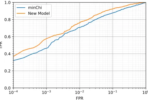
In figure 4 one can see a comparison of the ROC curves for one of the best performing variables in [1] and the MLP model. In this case only the events with 6 jets were used so the input length was fixed. The data used as background was QCD events with1500GeV≤H_partonT <2000 GeV. The MLP model used consisted of 4 hidden layers of 32 neurons with ReLu activation, with softmax activation on the final layer. The loss function was binary cross entropy and the model was fitted using the Adam optimiser[4]. The model was trained on 19801 events and tested on 11002 examples. The model was trained for 30 epochs with a batch size of 32. The log AUC score was 2.94 for the MLP and 2.73 forχ_min.

It is clear the MLP model is outperforming the variable here with an approximately 1% increase in log AUC score. This provides motivation for utility of NNs for classification of new physics events.

V. HYPERPARAMETER OPTIMISATION

Hyperparamter optimisation is an important part of developing any machine learning model. Many methods of hyperparamter optimisation exist. Two simple examples in common use are

10

10

10

10

10

FPR

0.0

0.2

0.4

0.6

0.8

TPR

minChi

New Model

FIG. 1. ROC curve showing performance ofχmin, and the MLP on data with fixed number of jets, in this case 6. Horizontal axis is log scale.

random search and grid search [3]. Random search consists of randomly selecting points in a bounded region of parameter space and evaluating them. The point with the best performance is chosen after N iterations. In grid search the bounded region is divided into a grid and points on the grid are evaluated. Although these methods are simple they are extremely easy to parallelise, allowing a large number of points to be evaluated quickly given sufficient computational resources. Bayesian optimisation is a an optimisation strategy that involves using Bayesian statistics to ex-plore parameter space in an efficient way[5]. Any Bayesian optimisation procedure consists of two main parts. First a posterior distribution over the parameters is calculated using all available eval-uations of target function. This is usually done using Gaussian process regression. The posterior is then used to construct at utility function, whose argmax is then the next point to be evaluated. Bayesian optimisation if particularly effective when the target function is costly to evaluate and the result of evaluation is noisy. This is the case when tuning the hyperparamters of a neural net-work as training and testing of a model takes time and resources, noise is an issue as training is a stochastic process. The usefulness of Bayesian optimisation as a strategy for hyperparamter tun-ing is exhaustively investigated in [6]. In this project the packagebayesian-optimization

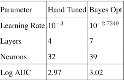
Parameter Hand Tuned Bayes Opt Learning Rate 10−3 10−2.7249

Layers 4 7

Neurons 32 39

Log AUC 2.97 3.02

TABLE I. Table showing the results of Bayesian optimisation of hyper parameters for the MLP model.

probability of improvement as the utility function[7].

The parameters optimised over were number of layers, number of neurons and learning rate. Bayesian optimisation using Gaussian process regression is only valid for continuous parameters, as this is part of the prior for Gaussian processes. There are various strategies for dealing with these discrete parameters as detailed in [8]. Here the method described as ’Basic’ in this reference was used. This is not optimal but avoids some of the pitfalls of ’naive’ rounding.

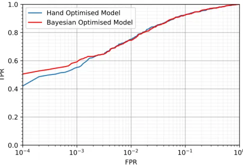
In figure 2 one can see the ROC curves for the network with optimised parameters and the previous best hand tuned network. The parameters that were optimised over were learning rate, number of layers and number of neurons per layer. All experimental parameters and data set were as in section IV. Thirty iterations of optimisation were carried out with 10 evaluations of the target function in parallel for each iteration. In table I the results of the optimisation are shown along with the log AUC score for each network. One can see that the Bayesian optimisation has marginally improved the score. The reason there is a not a very large improvement is probably because small networks with few hyper parameters such as this are reasonably easy to optimise by hand. As such the performance limit of this model was probably reached using optimisation by hand.

VI. EVENT WEIGHTING

The results in sections IV and V only consider background events in a smallH_partonT range. To provide a richer model of background events for the network to train on it is important to consider a wider range ofHT

parton. Care must be taken when extending this range however. Events with a low HT

parton have a much larger cross section than events with high HpartonT this means they are much more likely to occur in a real experiment . It is impractical however to generate simulated events with the frequencies with which they actually occur. For example a QCD event in500GeV< HT

10

10

10

10

10

FPR

0.0

0.2

0.4

0.6

0.8

TPR

Hand Optimised Model

Bayesian Optimised Model

FIG. 2. ROC curve showing performance of the models with paramters specified in table 1. Horizontal axis is log scale.

than a signal event. This means that to have a data set with a reasonable amount of signal events, one would have to have an unmanageable amount of lowH_partonT background events. There is also another issue with this large difference in cross section that is more specific to deep learning. If the data set is massively dominated by background events then any network will simply learn to classify every event as background.

Events in each HT

parton range are generated separately with approximately equal frequency to combat this problem . Events in rangeiare then assigned a weighting,wi, that is given by,

wi =

σi

Ni

, (3)

where σi is the cross section for events in that range, and Ni is the number of generated events

in that range. These weights are utilised later when assessing the performance of a network. For example when plotting a ROC curve these weights are used to calculated TPR and FPR. Usually when there is no weighting for a given classification threshold,

TPR= Nsel Nacc

, (4)

where Nsel is the number of events selected as signal, i.e. have a value greater than the given threshold andNaccis the number of events that are actually signal. When calculating the TPR with

FIG. 3. A diagram of the modified convDAN architecture used for variable length input data. weights included, TPR= P selwi P accwi , (5)

where the numerator is the sum over weights of selected events and denominator is sum over true signal events. The same principles can be applied to the FPR also. These weightings are not used to train the network, each event is presented to the network with equal weighting.

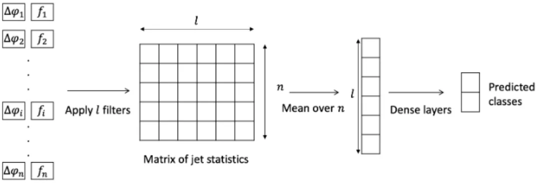
VII. CONVDAN

If a model is to be effective as a classifier of new physics events it must be able to accept inputs of variable length. This is because each event, in general, will have a different number of jets.

A typical model choice for one dimensional data of variable length would be a recursive neural network (RNN) [3]. This class of models has seen huge success in many areas, for example natural language processing. One feature of RNNs is that order matters, this is useful when considering speech for example, where neighbouring sections of the input are highly correlated. Our data how-ever has no natural order, as long as pairs off and∆φare kept together the data can be permuted any way and it will still describe the same event. Most NN models in fact place significance on the order of the input data, even the simple MLP model discussed in section IV. An architecture that ignores order must be used to properly reflect the structure of our data.

One of example of a deep NN model that ignores input order is the know as the Deep Averaging Network (DAN)[9]. This model was designed for sentiment analysis tasks in natural language processing. The input for a DAN is a set of n vectors of a fixed length, m, where n can vary between examples. In the first layer of the network the n dimension is averaged over leaving a

10

10

10

10

10

10

FPR

0.0

0.2

0.4

0.6

0.8

TPR

minOmegaHat

minOmegaTilde

convDAN

FIG. 4. The ROC curves for the convDAN, and the best performing variables from [1], with a full model of both EWK and QCD background, including weightings for differentH_partonT ranges. Note the extended FPR axis due to a larger data set when compared with previous figures

singlemdimensional vector. Sincemis fixed, this can then be used as an input to a standard feed forward network. In our casem= 2,f and∆φfor each jet, andnis the number of jets. Sincemis very small in our case when compared to a value of 300 used in [9], using this architecture would uneasily simplify the data at the first layer. For the reason a modification to the DAN architecture was made to better represent our data set.

In this modification a 1-dimensional convolutional layer is added to the start of the network. This layer applies a set ofl trainable filters to each 2D vector in the input. This can be thought of a set of statistics for each jet in the event. This yields anl×n matrix. Then dimension is then averaged over to give a vector of lengthl. This is then used as the input to a standard feed forward network. Because of the combination of a DAN with a convolutional layer this model is know as convDAN[10]. A schematic of the architecture used in the project can be seen in figure 3.

The ROC curve showing the performance of the convDAN can be seen in figure 4. 32 filters were used in the first layer of the network, each with 2 trainable weights and a bias. A ReLu acti-vation was used for these filters. The convolutional layer is followed by the averaging layer. After the averaging layer there were 3 fully connected layers of 16 neurons all with ReLu activation.

This was followed by an output layer with 2 neurons, with soft max activation. The model was again optimised with Adam, over 5 epochs with batch size 64. The network was trained on 688640 examples and tested on 147264 examples. Here the full set of both background and signal data was used including events with a range of jet multiplicities. It is clear that the network is consid-erably outperforming the hand designed variables over the entire range of FPRs. This network has a log AUC score of 3.42, a 19% improvement onωˆmin, the previous best hand designed variable. The jump in performance from the MLP could be explained by 2 factors. Firstly the size of the training set has increased dramatically. Secondly this model much better represents the underlying structure of the data. The second claim is supported when comparing the number of parameters the convDAN has with the MLP. The hand tuned MLP model has approximately 3 times the number of trainable parameters while its log AUC score is 14% worse.

VIII. SENSITIVITY

Although log AUC is a useful metric in this case it is not widely used by physicists to evaluate classifiers of new physics events. A much more common metric is what is known as the sensitivity. Calculating the sensitivity requires a full model of backgrounds and so EWK must be included in the data set. Sensitivity here is defined as the median discovery significance under the nominal signal hypothesis. A classifier with a higher sensitivity has a better chance of finding new physics. Note the term sensitivity is sometimes used as a name for the TPR, this is obviously not the case here. A popular way of approximating the sensitivity in a situation such as this (i.e. a counting experiment with know background) is to use,

med[Z0|1] =

r

2((s+b)ln(1 + s

b)−s), (6)

where s is the number of signal events classified as signal and b is the number of background events classified as signal[11]. Here we have that

s=X

sel

ws_i, b=X

sel

w_ib, (7)

where we are summing over the selected events andwb_{, w}s_{, represent the weights for true}

back-ground and signal events respectively. Equation 6 is derived and explained in detail in [11]. The underlying idea is the use of what is know as an Asimov dataset, which is an idealised data set that describes a given situation perfectly[11]. That is to say that any statistic calculated using this data

10

10

10

10

10

FPR

0.0

0.1

0.2

0.3

0.4

Sensitivity

train

test

minChi

minOmegaHat

min4Dphi

minbDphi

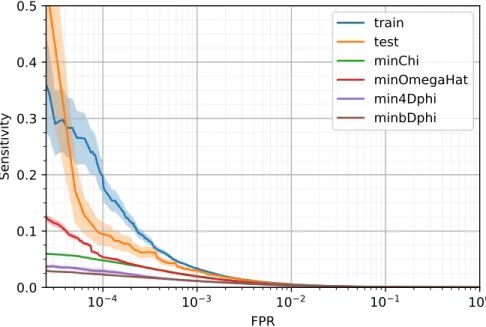
FIG. 5. A plot of the sensitivities of different varaibles, as the FPR is decreased. Shaded region is±1σ. χmin andωˆmin are the best performing variables from [1]. ∆φmin4 and∆φ∗_minare the variables currently used by CMS[13]. The performance of the model on the training and test set are shown for comparison.

set has a value equal to its true value. This formula can be modified to include some uncertainty in the value ofb, to give

S= [2((s+b)ln[(s+b)(b+σ 2 b) b2_{+ (s+b)σ}2 b ]− b 2 σ2ln[1 + σ2 bs b(b+σ2 b) ])] (8)

where S is the approximate sensitivity and σb is the uncertainty in b[12]. This uncertainty

rep-resents the experimental error, for example miss measurement in detector. Although our events are simulated, the detector response, including measurement error, is included as part of the sim-ulation, as such this uncertainty is present in our data. Note that this error is different from the statistical error in bothb ands. We can consider both b ands to be samples from a ’weighted’ Poisson distribution (if allw =1, sandb would be Poisson). The statistical error comes from the act of sampling from a random distribution. These errors can be propagated through equation 8 to give an estimate for the error inS, for a derivation, see appendix A.

In figure 5 one can see a plot of the sensitivity of the convDAN model compared to the previous best hand designed variables. The model here had exactly the same setup, both in hyper parameters and training as in section VII. A values of 15% ofb, was used forσb, the experimental error. It is

clear that the model is outperforming the variables by a large margin. One can see that as the FPR decreases the statistical error, consequently fluctuations in the sensitivity get larger. This is because in the low FPR region the threshold is very high and there are very few events above the threshold. As then there are less ’trials’, there are much larger fluctuations. The performance on the training set is included here for comparison. It can be seen that the sensitivity of the convDAN is higher for the entire region of FPR. The limitations of the data set size mean that FPRs lower than about 10−5 cannot be tested, it does however seem that the convDAN could increase its improvement on the variables in very low FPR region. The improvements on the variables is of such a size that even if the performance of the convDAN does worsen when the data set is modified to include manyHT

jetranges, which is not certain, it should still perform better than the variables.

IX. CONCLUSION

In this project we have presented evidence which illustrates the possible utility of deep neural networks in the classification of new physics events. A modified version of the convDAN archi-tecture has been presented, which represents the structure of our data well, particularly in that it ignores jet ordering and detects features on jet level. This leads to a large increase in performance when the deep model is compared to hand designed classifier based on the geometry of an event. This performance increase was seen in both log AUC score , and in a metric in more common use in experimental particle physics, sensitivity. The deep model has been shown to perform well on a varied data set of background and signal events, over a wide range ofHT

jet.

To fully complete this work there are a number of steps that must be carried out. Unfortunately it was impossible to complete them on this project due to time constraints. Theses steps include considering a wider range ofH_jetT and testing the network on a range of signal models. These steps can be seen in appendix B.

[1] Tai Sakuma, Henning Flaecher, and Dominic Smith. Alternative angular variables for suppression of QCD multijet events in new physics searches with missing transverse momentum at the LHC. 2018. arXiv:1803.07942.

[2] Andrew Ng. Machine learning yearning. 2017. URL:http://www.mlyearning.org/. [3] Ian Goodfellow, Yoshua Bengio, and Aaron Courville. Deep Learning. The MIT Press, 2016.

[5] Peter I. Frazier. A tutorial on bayesian optimization, 2018. arXiv:arXiv:1807.02811.

[6] Jasper Snoek, Hugo Larochelle, and Ryan P Adams. Practical bayesian optimization of machine learning algorithms. InAdvances in neural information processing systems, pages 2951–2959, 2012. [7] Fernando Nogueira. Bayesian optimization: Pure python implementation of bayesian

global optimization with gaussian processes. URL: https://pypi.org/project/ bayesian-optimization/1.0.1.

[8] Eduardo C. Garrido-Merchn and Daniel Hernndez-Lobato. Dealing with integer-valued variables in bayesian optimization with gaussian processes. 2017. arXiv:1706.03673.

[9] Mohit Iyyer, Varun Manjunatha, Jordan Boyd-Graber, and Hal Daum´e III. Deep unordered compo-sition rivals syntactic methods for text classification. InProceedings of the 53rd Annual Meeting of the Association for Computational Linguistics and the 7th International Joint Conference on Natural Language Processing (Volume 1: Long Papers), volume 1, pages 1681–1691, 2015.

[10] Andrew Gardner, Jinko Kanno, Christian A. Duncan, and Rastko R. Selmic. Classifying unordered feature sets with convolutional deep averaging networks, 2017. arXiv:1709.03019.

[11] Glen Cowan, Kyle Cranmer, Eilam Gross, and Ofer Vitells. Asymptotic formulae for likelihood-based tests of new physics. 2010. arXiv:1007.1727, doi:10.1140/epjc/ s10052-011-1554-0.

[12] G. Cowan. Discovery sensitivity for a counting experiment with background uncertainty, 2012. URL: http://www.pp.rhul.ac.uk/˜cowan/stat/medsig/medsigNote.pdf.

[13] CMS Collaboration. Search for top squark pair production in compressed-mass-spectrum scenarios in proton-proton collisions at sqrt(s) = 8 tev using the alpha[t] variable. 2016. arXiv:arXiv: 1605.08993,doi:10.1016/j.physletb.2017.02.007.

Appendix A: Error in sensitivity

To derive the error inSone can use the formula for error propagation, given by δ_S2 =δ2_s∂S ∂s 2 +δ_b2∂S ∂b 2 , (A1)

whereδS,δsandδb represent statistical uncertainties in,S,sandbrespectively. These derivatives

repository. Beacausesandb must be calculated using the weightings for events, findingδsandδb

is not necessarily as simple as just taking their root. sandbare really a weighted sum of Poisson variables, with one for each unique weight. The mean (and variance) of each of these variables can be estimated by the number of selected events in this weight class. Using the usual method for combining variances of a sum of random variables we obtain,

δs = s X sel (ws i)2, δb = s X sel (wb i)2. (A2) Appendix B: Steps

Below are the steps specified at the start of the project. It is hoped that the completion of all the steps would lead to publication quality work. In this work we have reached step 5.

1. Find an variable better than minChi on data with a fixed number (6) of jets. Only use one HT

parton range, single HjetT range, one signal model with specific parameters, only use QCD background. Use AUC as metric.

2. Develop model that works on variable number of jets, do better than minChi using data as above but with all jet multiplicities included.

3. Use QCD samples with differentH_partonT ranges, using weightings correctly. 4. Add electro-weak background, change metric to sensitivity.

5. Use multipleHT

jetranges, adjust sensitivity metric accordingly. 6. OptimiseH_jetT range boundaries.

7. Optimise number ofH_jetT ranges.

8. Test different parameters within one class of signal models, develop appropriate metric for this.