Who Needs Agglomeration? Varying Agglomeration Externalities and the Industry Life Cycle

0

Who Needs Agglomeration?

Varying Agglomeration Externalities and the Industry Life Cycle

Frank Neffke, Martin Svensson Henning, Ron Boschma, Karl-Johan Lundquist & Lars-Olof Olander

1

Authors

Frank Neffke*, Martin Svensson Henning#

Ron Boschma*, Karl-Johan Lundquist#, Lars-Olof Olander#

Version: March 2008

ABSTRACT

In this paper, the changing roles of agglomeration externalities during different stages of the industry life cycle are investigated. A central argument is that agglomeration externalities vary with mode of competition, innovation intensity, and characteristics of learning opportunities in industries. Following the Industry Life Cycle perspective, we distinguish between young and mature industries, and investigate how these benefit from MAR, Jacobs’ and Urbanization externalities. The empirical analysis builds on a Swedish plant level dataset that covers the period of 1974-2004.The outcomes of panel data regression models show that the benefits industries derive from their local environment are strongly associated with their stage in the industry life cycle. Whereas MAR externalities increase with the maturity of industries, Jacobs’ externalities decline when industries are more mature. This is in line with the hypothesis that young industries operate in an environment dominated by rapid product innovation and low levels of standardization. Hence, it pays off when knowledge can be sourced locally from many different sources, but there is still little scope for specialization benefits. Mature industries, in contrast, are associated with lower innovation intensities and a focus on cost saving process innovations. Therefore, there are major benefits to be derived from specialization, whereas knowledge spillovers from different industries are less relevant. The distinction between the product competition in young industries and price competition in mature industries is reflected in our finding that high regional factor costs are detrimental to mature industries, but not to young industries. This can also be related to the finding that high quality living environments, attractive for highly paid employees, are important to young industries. Overall, the outcomes stress that industrial life cycles have to be taken into account in the analysis of agglomeration externalities.

Acknowledgements

The authors gratefully acknowledge financial support provided by the Bank of Sweden Tercentenary Foundation and STINT (The Swedish Foundation for International Cooperation in Research and Higher Education) (Martin Svensson Henning); and NWO (Netherlands Organization for Scientific Research) (Frank Neffke).

*

Section of Economic Geography, Faculty of Geosciences, Utrecht University, the Netherlands. Correspondence: [email protected]

#

2

1. Introduction

A classical question in economic geography and regional economics is how geographic agglomerations contribute to performance of firms. In the externalities literature, it is a well-known argument that diversified cities offer different benefits compared to specialized cities (Jacobs, 1969). On the one hand, the diversity in knowledge spillovers and the quality and variety of the labour force are often greater in diversified metropolitan areas. On the other hand, factor costs are also usually higher due to crowding effects in the – usually larger – diversified cities. Specialized cities, in contrast, are commonly thought to offer easy access to industry-specific knowledge and a large specialized labour force. Firms in specialized cities can benefit greatly from the external economies of scale of the classical manufacturing cities. These scale economies are largely absent in cities without a clear specialization.

Since the seminal articles by Glaeser et al. (1992) and Henderson et al. (1995), a host of statistical-empirical studies have focused on the trade-off between diversification and specialization. Also many case studies have looked into this matter with renewed interest, most notably in the expanding literature on industrial districts and regional clusters (Asheim 2000, Porter 1990, 2000). However, the empirical evidence on agglomeration economies remains so far surprisingly inconclusive. The divergence in empirical results could be attributed to many factors (see e.g. Rosenthal and Strange, 2004; Smit, 2007). These range from differences across the industries, time periods to differences in geographic areas that are covered in different studies. Moreover, the different studies in the field display a large variety in the estimation framework applied.

The aim of this paper is to shed new light on this issue by establishing a link between the different types of agglomeration externalities that benefit firms and the life cycle stage of their industry. The main question we venture to answer is if the life cycle stage of an industry determines whether the industry will be most efficient if located in rather small specialized cities, or in large and diversified cities. To our knowledge, no study has yet systematically sought to explain part of the variation in benefits of agglomeration externalities by the use of a theoretical framework that links time and industry dimensions using a single, uniform database. We propose a theoretical framework that merges elements from the externalities literature and the Industry Life Cycle framework (ILC) (Gort and Klepper, 1982)). According to the ILC literature, industries develop along a stylized path from infant industries to mature or even declining industries. Along this path, shifts occur in three different dimensions: mode of competition, mode of innovation, and intensity of innovation. We claim these shifts have profound consequences for the influence of different kinds of knowledge spillovers and factor costs – and therefore for the effect of agglomeration externalities. Although the proposed framework is compatible with theoretical notions such as the “nursery cities” of Duranton and Puga (2001), and in line with the often stated conjecture that externality estimates for high tech industries will differ from low tech industries, to our knowledge the link between the ILC literature and agglomeration externalities has not yet been thoroughly described, let alone empirically tested.

Another contribution of this article is the proposed statistical framework, which tackles many of the difficulties that arise in empirical work in the field of agglomeration externalities. Most prominent among these are the Modifiable Areal Unit Problem (MAUP) and the problem of time-invariant regressors in panel data fixed effects models. In terms of the specification of the estimation model, we use a production function inspired approach, with value added as the dependent variable. In order to disentangle the effects of factor costs and knowledge spillovers, we use both agglomeration indices and variables capturing differences in factor costs across cities. The hypotheses are tested with data that cover life cycle stages across

3 twelve different industries in a panel of Swedish cities over the period 1974-2004. The empirical results show ample evidence for the link between the ILC stage and the strength of different types of agglomeration externalities. Our estimates show that young industries benefit from being located in high cost, high diversity locations. When moving towards mature industries, however, there is a gradual shift in benefits firms derive from regional externalities. Our outcomes show that mature industries are most efficient in low cost, specialized locations.

The structure of the paper is as follows. First, we briefly discuss the literature on agglomeration externalities. Next, we turn to the ILC concept and show how it may be used to structure our expectations on the strength of different types of agglomeration externalities. In section 4, we describe our dataset and explain how we determined the life cycle stages of the twelve industries. In section 5, we discuss the econometric specification and the empirical measurement of the theoretical concepts discussed in sections two. Section 6 describes the data and discusses the main results of our regression analyses. We conclude with an outline of our results and a discussion of further research.

2: Agglomeration externalities1

A typology

Agglomeration externalities can be defined loosely as benefits a firm derives from being located close to other economics actors (see for an extensive and general overview Rosenthal and Strange, 2004). Often a distinction is made between three types of externalities: Marshall-Arrow-Romer (MAR or localization) externalities, urbanization externalities and Jacobs’ externalities.2 In what follows, we will show how these types of externalities can be linked to opportunities for learning and the level of factor costs in a city.

Urbanization externalities are advantages experienced by firms located in large cities. For one, large cities offer access to high quality government and professional services. Metropolitan cities also often display a strong knowledge infrastructure. Major universities and research centres are often located in or in close vicinity of bigger cities. In this way, big cities generate advantages for firms as much as to the local labour force. Not only can employees get high level training in big cities, they can also more easily expand their knowledge by moving from one firm to the other and thereby enhance their skills and value to companies. Glaeser and Maré (2001) find that wages grow faster for migrants who move to big cities, indicating people accumulate skills and experience faster in large metropolitan areas. Another advantage of big cities is the size of the local market. This is not just limited to the large number of sophisticated and demanding consumers and firms to be found.3 Big cities are also hubs in large scale, international infrastructure networks. Therefore, firms not only benefit from a large local market, they also have easy access to other markets elsewhere.

!! "#$ % & ' ( ' ) * +!! , 2 # ' - - +!! , # ) ' ) . ) / 3 - 0 0 +1 ) !! , +!! , ) '

4 On the other hand, factor costs tend to be higher due to scarcity in big cities. Office space and land prices are also higher (Richardson, 1995). The higher wages that can be found in large cities not only reflect higher productivity of city dwellers, as firms also have to compensate their employees for the elevated costs of living inherent in city life. Furthermore, many negative externalities arise from congestion and pollution, which do increase costs to operate in cities, but are less readily translated into monetary terms. In sum, large metropolitan areas offer positive effects in terms of access to markets, knowledge and highly skilled employees, but they generally represent also higher cost environments than small cities do.

MAR externalities arise when firms benefit from a strong local specialisation in their own industry. A very early treatment of such externalities can be found in the works of Alfred Marshall (1890/1920), but they have received renewed attention within the urban economics literature, as well as in the industrial districts literature (for the latter see Asheim, 2000). In the Marshallian tradition, MAR externalities can be attributed to three sources: labour market pooling, input-output linkages and intra-industry knowledge spillovers. Benefits from labour market pooling arise because a large local industry is able to grow and sustain a highly skilled specialised labour force. In terms of know-how, this leads to a local expertise in the skills employed in the industry. At the same time, matching costs between employers and employees are lower (Duranton and Puga, 2004). High local concentration of an industry will also attract many specialised supplier and customer firms. This will help firms to economize on transport costs and minimize inventories. From the point of view of innovation, spatial proximity to suppliers and customers facilitates joint innovation efforts along the value chain. This is a rarely stressed observation in the discussion of MAR externalities, and relates to the third source of advantages of specialisation: local intra-industry knowledge spillovers. Learning processes as imitation and skill transfers are facilitated by face-to-face contacts which can be assumed to be more frequent between geographically proximate actors (Storper and Venables, 2004). In essence, we argue that, in many ways, MAR externalities are associated with processes of localized learning and the transfer of specialised knowledge on the one hand and cost savings through external economies of scale on the other hand.

In contrast to MAR externalities, Jacobs’ externalities arise when firms benefit from the local presence of a high level of industrial diversity. Local diversification provides scope for combining knowledge across industries (Jacobs, 1969). Frequently, industries face problems that have close analogues in other industries. Solutions that are applied in one industry can in these cases often be readily adapted to solve problems in other industries, and a firm located in a city with a large variety of industries can therefore draw on a large and varied local “problem solving database”. Moreover, a diversified regional economy increases the chances of unexpected inter-industry knowledge and product combinations to arise.

However, these are not the only advantages provided by diversified cities. Industrial diversity creates stable demand and supply conditions as well. Firms are less likely to be hit by strong negative demand shocks if sales are distributed across a higher number of different local industries. Moreover, when firms are able to choose from a wide range of local input substitutes, exposure to price fluctuations in single input varieties is reduced. Related to this argument is the love of variety argument in Dixit-Stiglitz production or consumption functions (Dixit and Stiglitz, 1977). These models show that if firms can switch easily between input varieties they experience lower production costs when operating in diversified cities (e.g. Duranton and Puga, 2004).

Although congestion and high factor costs in large diversified cities may give rise to negative externalities, diversity per se – as explained above – is generally thought to benefit local industries. However, some empirical studies showed that diversity has a negative effect on

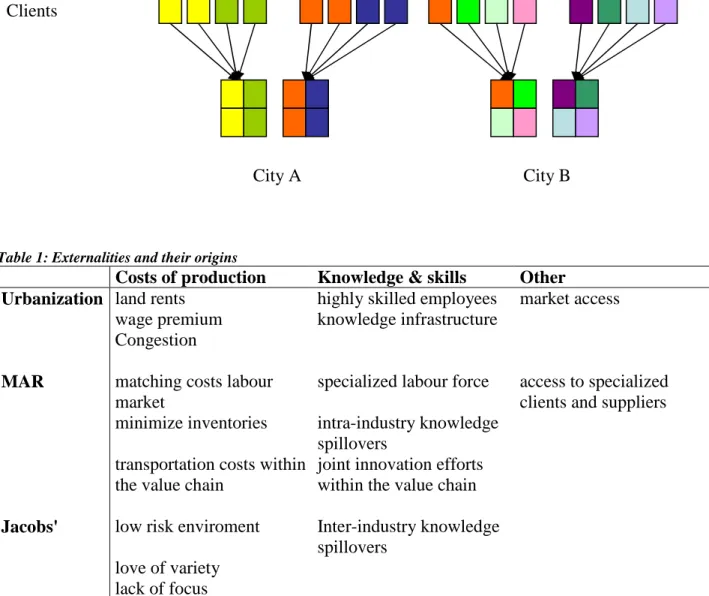
5 local economic performance. Often these outcomes are treated as “perverse” and largely ignored. For instance, Henderson (2003) finds that diversity has a negative effect on firm performance in some industries, and Combes (2000) finds negative effects for heavy manufacturing industries. In both studies, these findings are mentioned without probing into their meaning or causes. In contrast to these studies, we argue that Jacobs’ externalities may turn negative if they lead to a lack of focus in local general services. By general services we mean services that are shared by firms belonging to different industries. They include both professional producer services like accountancy and marketing agencies, and public services such as transportation networks and educational facilities. Small and medium sized cities can only sustain a limited number of suppliers of these services and local governments can tailor their services only to a limited number of industries. As a result, cities that host a lower variety of industries can offer more specialized general services. Figure 1 shows the situation for two small cities of equal size that have just enough economic activity to provide business for two marketing agencies.4 The squares in the upper part are the client firms, with different shadings for each industry. The squares in the lower part represent the service providers. In city A, each agency can specialize on the provision of services for two industries, and can therefore become fully acquainted with the specific demands of those industries. In contrast, in city B, each agency needs clients from four different industries in order to generate sufficient income. For marketing agencies in city B, it is therefore much harder to offer the same level of tailor made services to their clientele than for those in city A. This lack of focus in city B may lead to higher production costs due to lower quality general services, which will be especially important when the demands of industries are rather specific, and do not change too much over time so service providers have the opportunity to adapt.5

-Figure 1 about here-

Table 1 summarizes the different sources for urbanization, MAR and Jacobs’ externalities. The rows correspond to the different externality types and the columns differentiate between factor costs and knowledge spillover origins of the externalities.

-Table 1 about here- Empirical findings

Since the seminal article by Glaeser et al. (1992), the statistical-empirical literature investigating the distinction between MAR, Jacobs’, and urbanization externalities has expanded rapidly. Unfortunately, though, this has not led to a full understanding of the matter. Instead of an accumulation of evidence on the strength of MAR, Jacobs’ and urbanization externalities, outcomes vary frantically across studies. For example, Feldman (2000) notes in a literature review about the connections between innovation and location that there is wide 4 " 2 ) - 3 0 4 5 +6 7,) . 8. 2 '+..2, ..2 ) / 0 )

6 divergence between the empirical results on the importance of localization economies. Glaeser (2000) reaches similar conclusions when it comes to the difference between the impacts of concentration and diversity respectively.

A reason for the lack of convergent outcomes may be that studies differ widely in their set-up. On the one hand, there are differences in methodology along a number of axes: plant level versus regional studies, panel data versus cross-section analyses, and productivity versus employment regressions. On the other hand, samples cover a wide range of different periods in history and relate to different geographic areas in the world. Smit (2007) has reviewed 31 studies containing over 200 parameter estimates. In a meta-regression, he finds that sample issues as well as methodological issues affect outcomes. Also Neffke (2007) found that the outcomes reported in seven leading articles were subject to extensive variation, even for studies that focused exclusively on the United States. In a study of all local manufacturing and service industries in French labour market regions by Combes (2000) parameter estimates on urbanization, MAR and Jacobs’ externalities ranged from negative and significant to positive and significant. Especially contentious is the role of Jacobs’ externalities. While Glaeser et al. (1992) and Henderson (2003), in general, did not find consistent effects of a diverse local environment, Rosenthal and Strange (2003) did find diversity benefits, and Henderson et al. (1995) reported a positive influence on the formation of high tech industries.

The latter study by Henderson and his colleagues suggests that industries have some general characteristics that may help explain whether a specialized or rather a diversified city caters most of its needs. Referring to a Vernionian product life cycle view of regional development, it is often hypothesized that product development takes place in big, diversified cities, whereas production takes place in smaller yet specialized cities (e.g. Henderson 2003; see also Lundquist and Olander, 1999). Duranton and Puga (2001) formalize this conjecture in their “nursery cities” concept. We agree with the idea that specialized cities may be attractive for different industries than diversified cities. As a matter of fact, in this article we hypothesize that a part of the variation in externality estimates can be predicted by considering how industries differ from one another. Nevertheless, we will argue that it is important to consider general aspects of industrial development as described in the industry life cycle literature. Prominent among these are the evolution of market structure and changes in innovation processes, which may have profound effects on which types of regional externalities are most important to industries. By sticking to one general econometric approach for all industries in our study, we aim to isolate the effects of movements of industries along the industry life cycle on the size and sign of agglomeration externalities.

3: Industry life cycles and agglomeration externalities

The ILC framework

The industry life cycle framework (ILC) (Gort and Klepper, 1982; Abernathy and Clark 1985; Klepper 1997) is a stylized description of the evolution of an industry from infancy to decline. The archetypical evolution of the output in an industry follows a logistic (or S-) curve, starting with the introduction of a new product6 (introduction or infancy phase), followed by a period of strong expansion of production (growth phase), which levels off (maturity or stagnation phase) and eventually decreases (decline phase). The ILC literature has grown into an extensive body of articles with many detailed descriptions and subtleties. In this paper, we are

6

3 )

7 mainly interested in three aspects of the industry life cycle stages: type of innovation, innovation intensity, and mode of competition.

The birth of a new industry typically follows from radical innovations that result in new products. The early stages are characterised by the development of an immature technology. Large discontinuities in a technological sense in this stage are not uncommon – innovation is of a radical nature – as standardization has not yet occurred. Therefore, as argued by Gort and Klepper (1982), information about the innovation(s) can come from a wide range of sources in these stages, often from outside the young industry’s population of firms. Moreover, innovation intensity and success are high, as there are still many unexplored technological opportunities. As experience has yet to build up, knowledge about the production process is uncertain, and therefore easily acquired. This leads to low barriers to entry. Attracted by the promise of unexploited innovation opportunities and the associated high profit margins, start-ups and other entrants to the new market are numerous. Due to the typically small scale production and large diversity in product designs, the predominantly young firms compete on the basis of quality characteristics of their new products.

The turning point of industry development is the establishment of a ‘dominant design’ within an industry (Utterback and Suárez 1993). The dominant design allows production to become more standardized, which opens up possibilities for firms to exploit division of labour and economies of scale. Companies are in this stage producing more or less similar products and get increasingly involved in price competition. This leads to a sharp drop in prices, which greatly enlarges the client base from the early adopters to a wider general public. Output volumes go through a period of steep growth. In terms of innovation, longer jumps in technology are less likely. The components of the production process become ever more adapted to each other, and innovations are more incremental in nature. Emphasis will turn more towards process innovation, and the main focus will be increasingly directed to efficiency gains. Generally, this kind of innovation requires very specialized, industry specific knowledge, skills and machinery. Due to these developments, and the expanded scale of production, barriers to entry rise and the number of entrants declines (Gort and Klepper 1982). In the following stage, the industry reaches its maturity. Firms typically face vigorous price competition. Profit margins are reduced and technological opportunities get exhausted (Gort and Klepper 1982). This is reflected in a low innovation intensity. Moreover, radical innovations are all but infeasible, as the industry has invested heavily in machinery and skill development that would become obsolete by dramatic discontinuities in technology. If the industry is not able to reinvent itself as it approaches the late states of maturity, it will proceed into decline, producing the same amount of output with ever fewer employees, lowering other production costs and moving production plants to low wage locations (Perez and Soete, 1988). Table 2 summarizes how an industry changes when moving from a young to a mature stage.

-Table 2 about here-

Generally, a complete life cycle spans a long period of time: its individual stages often cover many years. However, the ILC description of industry development is highly stylized. In practice, industries could rejuvenate after a radical innovation that has far reaching consequences on the industry. In this case no new industry arises, but the new technology opens up new technological opportunities and designs, and lowers barriers to entry. This effectively brings the industry back to infant-like stages. Nevertheless, the work by Gort and

8 Klepper shows that the ILC works remarkably well across the 46 different industries they investigated.

Changing agglomeration externalities along the industry life cycle

As discussed in section 2, agglomeration externalities matter to the economic success of local industries. However, it is the pivotal argument of this paper that their strength depends on factors that are related to the industry life cycle. 7 The higher factor costs associated with urbanization externalities, to start with, will be detrimental for mature industries as they have to compete on price. However, young industries are far less affected by factor costs differentials. They mainly engage in competition based on quality differences in product varieties. Better access to knowledge and a highly educated labour force is often crucial for the development of those varieties. Mature industries, in contrast, have less demand for expensive, highly educated employees in their large scale production facilities. For similar reasons, they do benefit much from the access to large markets, whereas young industries benefit from the interaction with sophisticated early adopter-customers in big cities.

MAR externalities also generate cost savings and therefore benefit especially mature industries. They also derive great advantage from the labour force in cities with MAR externalities. This labour force is not necessarily highly educated, but very specialized. The incremental innovations that take place by learning by doing and imitation in specialized environments like traditional industrial districts (Amin, 2003) fits the profile of mature industries very well. In young industries these advantages exist as well, though to a lesser degree, as the tasks that are performed still lack the required level of routinization (e.g. Nelson and Winter, 1982). For the same reason, the standardized technologies used in mature industries lend themselves far more to the orchestration of innovation efforts along the value chain than the constantly changing technologies used in young industries. This also limits the extent to which young industries will be able to build up strong and long-lasting buyer-supplier networks.

The inter-industry knowledge spillovers associated with Jacobs’ externalities are of utmost importance to young industries. These industries need and can accommodate a large variety of knowledge and use it to build superior products without having to completely refurbish expensive, large-scale production facilities that are used in mature industries. Similarly, this flexibility in the production processes of young industries puts them in a position to use a larger variety of input alternatives. The uncertainty about market conditions arising from unfamiliarity with and diversity in the products of young industries, puts another premium on local diversity. This may be absent for more mature industries with standardized products. Young industries, however, are usually not sufficiently embedded in the local environment to benefit from possibilities to lobby for a strong focus on their business interests with the local business service providers and the local government. In early stages of development, the needs of these industries will not be known to policy makers, and local service supply and policies need time to adapt. This contrasts strongly with mature industries that over time have developed strong ties in the region. Firms operating in mature industries in diversified cities

7 _{Our view shows similarities to}

a regionalized version of the Vernonian product life cycle, see Lundquist (1996).. In the 1980s, the ILC approach was widely applied in economic geography to explain the rise of new industries in new growth regions that were different from the ones where the more mature industries were located and in decline (Norton, 1979; Norton and Rees, 1979; Markusen, 1985; Scott, 1988; Davelaar, 1989, Storper and Walker, 1989; Boschma, 1997). This literature emerged against the background of the rise and growth of the so-called Sunbelt states that were located outside the main manufacturing heartland of the US. Audretsch and Feldman (1996) extended the ILC theory to the tendency of spatial clustering, finding evidence that the propensity of innovative efforts to cluster spatially was shaped by the characteristics of the life cycle phases.

9 may, therefore, find it hard to compete with firms in more focused cities. The latter have often been able to tailor the local education system, infrastructure and many other aspects of the local environment to their specific needs (Grabher, 1993).8

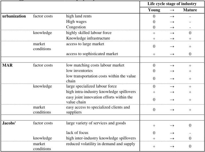
Table 3 merges the elements of table 1 and 2 to summarize this discussion about the interplay of agglomeration externalities and life cycle dynamics. In the rows, the externality types and their different sources are listed. In the columns we show how the influence on the competitiveness of local industries (negative, no effect, or positive effect) changes when moving from young industries towards mature industries.

-Table 3 about here-

4: Data and industry life cycle stages

Database

The data used in this study are taken from a dataset that contains employees, value added (VA) and location data for all Swedish manufacturing plants with five employees or more (1968-1989) or with at least five employees pertaining to firms employing at least 10 people (1990-2004). 9 All plants in the dataset are classified according to the Swedish SNI-code system at the five digit level (similar to the SIC classification). Due to a change in this system, we had to merge some of the five digit industries. This resulted, for those industries, in classes that lie roughly between the three and four digit level.10 The geographical location of plants is known at the municipality level (there are 277 in our dataset).11 This provides us with a high quality database containing very detailed information about the development of the Swedish economy from the late 1960s up to this date.

Calculation of potentials

As the unit of our analysis is the local industry, we must aggregate plant level data into spatial units. A classical problem occurs when simply summing micro-level data up to regional units: outcomes of analyses based on such data are often subject to change when borders of units are redrawn. Moreover, there are many qualitative differences between regional units. For one, some regions are larger in terms of area than others. Another issue is that some regions are multi-core regions, whereas other regions are dominated by one large city. In this study, we argue that agglomeration externalities are primarily found in cities. Swedish municipalities are, in many cases, too small in terms of population12 to exhibit the kind of agglomeration externalities discussed in the literature, which originally focused on metropolitan areas only (e.g Glaeser et al., 1992).

8 # ) +!!;, ) - - 2 ) 2 ) ) 9 # ) 3 . +6 9, 3 3 10 ) ) ) ) ) ' 11

We have run several algorithm-based data cleaning procedures and parts of the data were checked by hand 2

6

10 For these reasons, we construct metropolitan area data around Swedish labour market regions (so-called functional or A-regions). In total, Sweden consists of 70 such regions, most of which are dominated by a single large city. Nevertheless, some harbour two or more core cities of more or less equal size. It is unlikely that these regions experience the same magnitude of agglomeration externalities as regions with a similar population, but concentrated in a single core. However, if the cities in the multi-core region are not too far apart, total agglomeration externalities in each city should exceed the ones that are to be expected on the basis of only its own population and firms. In sum, simply attributing all economic activity to a single point in space would overstate the size of externalities, whereas focusing only on the largest city would understate them.

Instead of committing ourselves to one of these extremes, we use our data to calculate potential measures for the largest cities in each of the 70 labour market regions in Sweden. The first step we take is to find the largest population centre for each municipality. We shall call this the municipality-capital. A municipality typically consists of one major core and a number of villages that are an order of magnitude smaller. Therefore, we assume that all economic activity takes place at the location of this core.

Next, we find the largest municipality-capital of a given A-region and call this the “A-region-capital”. We calculated the road distance from each A-region-capital to each municipality-capital. This distance matrix was then used to build a spatially weighted sum of all contributions from all municipalities, which gives us the A-region-capital’s potential. There is one drawback in this approach. If we were to apply the potential-calculations as described above to the dependent variable of a regression analysis, we would artificially create spatial autocorrelation. Therefore, when calculating potentials for the dependent variable and the scale variable (see below), we set all contributions of municipalities outside the A-region equal to zero. Take for example the number of plants. Let:

mit

P : number of plants in municipality m∈M in industry i at year t. ma

d : road-distance between the capital of municipality m and the capital of A-region

A a∈

M: set of all municipalities in Sweden

A: set of all A-regions in Sweden

Now the “plant-potential” in industry i for A-region-capital a is calculated as follows:

(

)

∈ = M m mit ma pot ait f d P P

δ

,

(

dma

)

f

δ

, is a distance decay function13. Analogously, we can calculate a population-potential, an employment-potential and a valued added-potential for each of the 70 cities. To the data we derived from our plant database, we add municipality data on population and house prices, acquired from Statistics Sweden.14 For population data we again calculate ; ' < -) - ( ) - #8 8 ) 0 8 - #8 8

11 potentials. The house price indicators, however, are not spatially weighted and reflect the house prices in the capital-cities.

Industries and lifecycles

In total, our sample distinguishes between 102 different industries that can be followed consistently over time. However, most of the industries are very small and only present in a handful of labour market regions. As this would cause additional estimation problems, we focus on 12 major industries that have a presence in most parts of Sweden. These 12 account for some 44% of total Swedish manufacturing output in 1974 and for 42% in 2004, and therefore cover a large part of the Swedish manufacturing sector.

A major challenge is to find an adequate way to determine the life cycle stages of each industry in time. Gort and Klepper (1982) use a method that relies on the differences in entry and exit dynamics between the stages. A problem with this method in our study is that the Swedish market is very small compared to the US market. Although each industry is composed of many plants, entry and exit in absolute terms is small and therefore rather volatile in relative terms. A more fundamental issue is the influence of business cycles. In the short run, much of entry and exit dynamics are a result of overall performance of the economy. For these reasons, we have turned to a different method to identify life cycle stages. Our assumption is that the stage of the life cycle can be determined by looking at the age of plants in the industry. Technology is to a large degree embedded in machinery, which is costly to replace. More importantly, however, to adopt new technologies routines must be adapted. It is quite commonplace that firms struggle very hard to accomplish this (Nelson and Winter, 1982). For both reasons, we argue that old plants generally use older technologies than young plants, as the latter can choose the machinery and build routines according to the best available technology at that moment (Davelaar, 1989). If an industry is in a stage of strong technological renewal – i.e. if the industry is young or rejuvenated – the young plants should be able to capture large shares of the market from the older plants. In contrast, if the industry is in a stage with a stable technological trajectory, older plants are less threatened by new entrants and will retain a larger share of the market.

The argumentation above suggests that we can determine the level of maturity of an industry by looking at the market share of old plants in an industry. Defining old plants as plants of 10 years and older, we have calculated this for all industries in our database. However, we would like to control for the fact that economy-wide plant turnover may have increased (or decreased) over the decades. Therefore, we divide the old-plant market shares of each industry by the market share of old plants in the economy at large. This yields an index that represents the over or under performance of old plants compared to the national level. Next, we normalize this index by subtracting the mean (which is equal to one) and dividing by the standard deviation across all industries. Let the maturity index be:

tot t old t tot it old it it

VA

VA

VA

VA

I

=

Where: 14 + 8 ) ' ,) 3 3 = ! ) > + , ? ) !@7 !

12 old

it

VA : value added in old plants in industry i at year t tot

it

VA : value added in all plants in industry i at year t old

t

VA : value added in all old plants in Sweden at year t tot

t

VA : value added in all plants in Sweden at year t The normalized maturity index is now:

( )

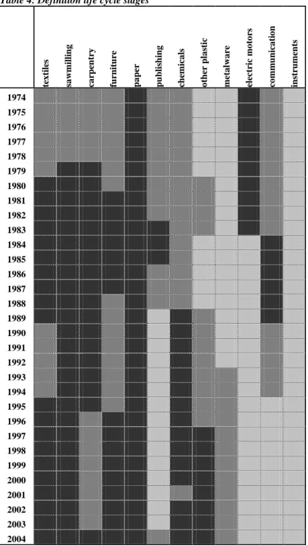
it it norm it I stddev I I = −1

We distinguish between three types of maturity: young, intermediate and mature. In order to obtain a roughly equal number of observations for each type, we use as a cut-off value for the normalized maturity index of .3. According to this definition, industries are young if their maturity index is lower than -.3 standard deviations than 1. Intermediate stages have maturity indices that are between -.3 and +.3 standard deviations from 1. For maturity indices greater than 1 + .3 standard deviations, the industry is considered to be mature. Using a five-year moving average to control for business cycle volatility, table 4 shows for each year the life cycle stages for the twelve industries of our study. As the figure displays, the trajectory of an industry could consist of different stages. For example, other plastic shows young as well as intermediate and mature stages. However, it is important to note that industries may shift repeatedly from one category to the other, because their maturity index is most of the time close to the threshold.15

-Table 4 about here-

The general picture shows that, in line with general intuition, textiles, sawmilling, carpentry, furniture, paper and chemicals have been rather mature industries over the course of the entire past three decades. The signs of rejuvenation in the 1990s for communications are supported by the literature (see Schön, 2000). Another industry that undergoes rejuvenation in the 1990s is publishing. Electric motors enters a young stage already in the 1980s. Other plastics, in contrast slides into maturity. To a lesser degree, the same holds for metal ware. The instruments industry has been classified as a young industry for all years in our sample.

5: The regression equation and econometric issues

In order to measure the size of externalities, we estimate a Cobb-Douglas inspired production function for city-industries. Output is measured by value added. Unfortunately, due to a lack of capital data, the only inputs in the production process at our disposal are employment data. This gives rise to the following multiplicative model:

+, VA_cit =T_citLα_citε_cit

where: 9 15 # ) - 9 9 = )A# ) ) ' ) & #8

13 cit VA B A cit L B C cit T B '

We will now turn to the elements that make up the technology term. A good first proxy for the size of urbanization externalities is the population potential:

(

)

∈ = M m mt mc ct f d pop pop

δ

,

However, we would like to empirically disentangle the different sources of urbanization externalities that we discussed above. We therefore control for two other factors. The first is the overall wage level in the city. We calculate this as the relative wage level in a city compared to the national wage level, while controlling for sector composition:

= i it cit ct cit ct w w L L wage B it w B 3

This results in an index that is equal to one if the weighted average wage across industries in a city equals the average national wages for a matching industry structure. This variable captures both differences in quality of the labour force and variations in the cost of living in different cities. Our aim, however, is to isolate the latter effect. For this purpose we use the house price index (housect). As the rents account for a large part of the expenditures by households, the higher costs of living in big cities reflected in higher wage levels are to a large degree captured by the house price variable. For this reason, the wage index will be assumed to reflect mostly differences in quality of labour.

MAR externalities have been modelled in various ways in the literature. Levels or shares of own industry employment are widely used indicators (e.g. Glaeser et al., 1992, Henderson et al., 1995, Henderson, 1997). However, these indicators do not differentiate between plant internal and plant external economies of scale. In the extreme case where all the employment in a city-industry is located in a single plant, the effects level of local employment would be fully attributable to internal economies of scale. Therefore, as argued above, we use the labour potential, as a measure for the local scale of inputs in the industry. The number of plants can, by construction, only give rise to external economies of scale. We therefore measure MAR externalities by the potential of the number of plants in the local industry:

(

)

∈ = M m mit mc cit f d P MAR

δ

, B mit P B )

14 Henderson (2003) argues that each plant can be interpreted as an experiment with a specific variation on the production process of the industry. Intra-industry knowledge spillovers are more numerous when there are more of those experiments in the immediate vicinity. Similarly, one can argue that workers acquire more industry specific skills by moving between a large number of plants than by the mere size of the labour force. A large number of plants also results in more potential innovation partners in the own industry. However, lower matching costs and savings in transportation and inventory costs are not immediately reflected in this variable.

The index measuring Jacobs’ externalities should reflect the presence of a large diversity of industrial activity in a city. For this purpose, many authors use an index that focuses on the distribution of economic activity across the different local industries, like the Hirschman-Herfindahl index (HHI) or the entropy index of local industries’ employment shares. However, the disadvantage of these measures is that they do not capture the essence of Jacobs’ externalities. A distribution with three major industries but no other industries can result in the same entropy or HHI as a distribution with one major industry and a number of equal-sized but negligible industries. However, the first situation is more likely to give rise to spillovers or inhibit focus than the second. The number of significant industries in a city is therefore a more adequate measure. We call an industry’s presence in a region significant if its size reaches a certain threshold.17

(

)

≥ = ∈ i m M mit mc ct g f d P JAC

δ

, 10 B

()

. g B

Here we base the Jacobs’ externalities indicator on the number of plants potential. As for the MAR externalities, we argue that the number of experiments that take place in different plants are most relevant.

Assuming that all externalities and control variables enter the technology term in a multiplicative way, we can arrive at the following log transformed estimation equation:

+6,

(

)

( )

(

)

(

)

(

)

(

cit

)

(

cit

)

( )

cit

ct ct ct cit cit JAC MAR house wage pop L VA

ε

β

β

β

β

β

α

log log log log log log log log 2 5 2 4 3 2 2 1 + + + + + + = − − −

As the effects of local learning will only be felt after a certain amount of time, we have lagged all variables that mainly capture knowledge spillovers by two years.19 The major contribution 17 ) # ) ' )

( )

Lcit log / B

(

) (

) ( )

(

)

(

)

(

)

(

cit

)

(

cit

)

( )

cit

ct ct ct cit cit cit JAC MAR house wage pop L L VA

ε

β

β

β

β

β

α

log log log log log log log 1 log 5 4 3 2 1 + + + + + + − = )

α

8 ) ' 19 D /

15 of this study is that we investigate how externalities differ between life cycle stages. To accomplish this, we pool observations across all industries and make coefficients dependent on the particular life cycle stage. We use a panel model to estimate these parameters. As productivity may differ strongly across industries, we control for industry-city fixed effects. This also controls for all unmeasured time invariant city variables. Prominent among these are geographical aspects, like locations with access to the sea and institutional differences across regions. Moreover, to control for factors that influence the entire Swedish economy in one year – as for example inflation and business cycle movements – we also add year effects. This results in the following final specification:

+;,

(

)

( )

(

)

(

)

(

)

(

)

(

cit

)

ci t

( )

cit s cit s ct s ct s ct s cit s cit JAC MAR house wage pop L VA

ε

δ

η

β

β

β

β

β

α

log log log log log log log log 5 4 3 2 1 + + + + + + + + = where: ci

η

: industry-city fixed effects

t

δ

: time invariant city variables

6. Empirical results

The Swedish geography of young, intermediate and mature industries

= )

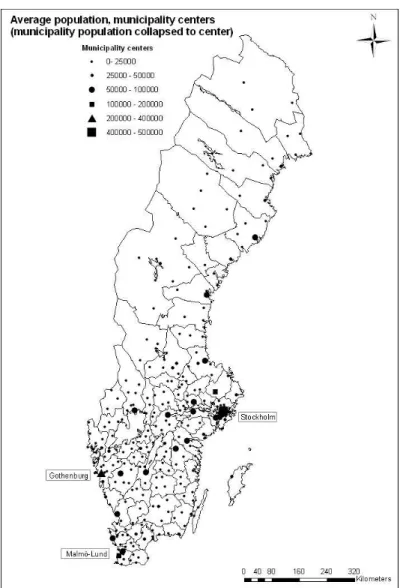
To give the reader an overview of the empirical context in which our study is situated, we have included some descriptive maps. In figure 2, the average population of the municipalities over the years of the sample is displayed. The largest agglomerations are in the Stockholm, Gothenburg and Malmö/Lund areas. Stockholm had about 1.9 million inhabitants in 2006, as compared to 9.1 million in the country as a whole. The north of Sweden is scarcely populated, except for some major cities along the coast. This unequal spread of population underscores the importance of the spatial weighting scheme we adopt. Figures 3-5 display average percent of value added in the regions for young, intermediate, and mature industries. The young industries are clearly concentrated in the major regions, with an emphasis on the Stockholm region. Other large parts of the young industries are located in university regions around the country, like Malmö/Lund and Uppsala. As shown in Figure 4, the intermediate industries are more scattered, and widely represented both in the major population centres and in more peripheral parts of the country. However, these industries also show strong presence in the traditional small-firm districts in the south-western parts of the country. Figure 5 shows that the value added of the mature industries is produced in a wide range of different regions. The focus shifts much more to the periphery and more traditional heavy-manufacturing regions in Mid-Sweden and along the coast of northern Sweden. Mature industries are more equally distributed across space than young industries, as reflected in the Gini-coefficients.

Figures 6-8, finally, display average labour productivity in the different sectors. The indicators have been normalized, so that a value above 1 indicates a superior productivity over the national average. For young industries, labour productivity is rather similar across the different regions, with clear exceptions in the Stockholm, Linköping (a mid-sized university city), and some regions in more peripheral locations. The intermediate industries show a more diffuse pattern, and the regional variations in productivity are not as large as for the young

16 industries. In the case of mature industries, large metropolitan regions are in general not the most efficient ones. For these industries, high efficiency can typically be found in more peripheral locations all over the country.

-Figures 2-8 about here-

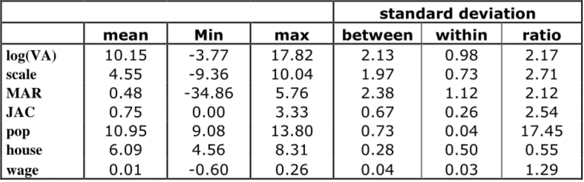
Table 5 shows the main descriptive statistics for our dependent variable, log(VA) and for the six regressors. Table 6 contains the correlations between the regressors.

-Table 5 about here- -Table 6 about here-

Baseline and some basic estimation issues

As a baseline, we estimate the effects of externalities without distinguishing between life cycle stages using a LSDV, or fixed effects, estimation. The outcomes are shown in column (1) of table 7. In this specification, the scale variable is very close to 1, indicating constant returns to scale. MAR externalities are positive and have an elasticity of the order of 2%, meaning that a doubling of the number of own industry plants leads to efficiency gains of 2%. As a comparison, this estimate ranges from 2% to 8% in Henderson (2003). Jacobs’ externalities seem to be absent. The point estimate of urbanization externalities, as measured by population, is high, but the standard error is large as well. Looking at table 5, it becomes clear why this is the case. The population of a city changes only very slowly over time, which gives rise to a very low within standard deviation. However, the between standard deviation is very high as, cross-sectionally, population potentials vary widely. The fixed effects estimator only makes use of the within variation in the sample. This leads to inefficient estimates of the population parameter. Including the extra information in wages and house prices (column 2, table 7) unfortunately does not solve the problem. In this specification, all urbanization related variables have insignificant effects.

A way to get a better estimate on the population parameter is using random effects. The random effects estimator is a weighted average of the fixed effects estimator and an estimator that is based on the cross-sectional variation in the sample, and it is therefore able to exploit both the within and the between variation in the regressors. However, this comes at a cost, as the random effects models assume that the unobserved city-industry fixed effects are uncorrelated with the regressors. Theoretically, there is little reason for this assumption, but column (3, table 7) nevertheless presents the results. The population estimate is now small, but negative and the standard error has dropped tremendously. The other parameter estimates have remained more or less the same. However, a Hausman test on the adequacy of the random effects model is significant at any conventional level. This clearly rejects the random effects specification. We therefore cannot assume that regressors and city-industry effects are uncorrelated.

We are confronted now with a predicament: on the one hand, fixed effects will not allow us to get precise estimates on one of our core variables, on the other hand, random effects have not passed the Hausman test. Theoretically, the Hausman-Tailor procedure (Hausman and Taylor, 1981) could be applied. However, the fact that for this method one has to find variables that

17 can be convincingly thought of as a priori uncorrelated with the city-industry effects, makes this method problematic (Arellano, 2003, p. 44).

A different solution has been developed Plümper and Troeger (2007). They use a procedure in steps that was originally proposed by Hsiao (2003)20. The methodology developed by Plümper and Troeger, called the “Fixed Effects Vector Decomposition” (FEVD) method, gives rise to unbiased estimates for the variables that have been identified as time-varying. The drawback is that the estimates of the effect of time-invariant and slowly changing variables are biased, as already noted by Hsiao (2003). This bias depends on the correlation between the time invariant and slowly changing variables and the unexplained city-industry effect.21 As the city-industry effects are unobserved, it is impossible to assess this correlation. However, Plümper and Troeger show that for a wide range of values for the correlation, in small samples, the FEVD estimator outperforms the FE, RE and Hausman-Taylor estimators in terms of the Root Mean Squared Error (RMSE). This means that, although the estimates maybe biased, the bias is small and the increased efficiency more than compensates this in most cases.

In our study, the superiority of the FEVD depends on two things: first the correlation between the city-industry effects and the regressors that we regard as slowly changing, and, second, the ratio of between to within standard deviation of the slowly changing variables. Looking at tables 5 and 6, population is clearly a slowly changing variable, with a between-within ration of over 17.22 As pop is strongly correlated to JAC and a large part of the variation in JAC is actually cross-sectional, omitting JAC from the residuals would give rise to a large omitted variable bias in the second step of the FEVD procedure.

Column (4) in table 7 shows the estimates for an FEVD specification where pop and JAC are modelled as slowly changing variables. The estimates are similar to the RE estimates. The time-varying variables, scale, MAR, house and wage, are all indistinguishable from their FE estimates in column (2). However, there are three main differences between the FE and RE estimates, on the one hand, and the FEVD results on the other hand. First, Jacobs’ externalities are significant and negative. Next, the parameter for population is positive and for the first time significant, but very close to the RE estimate. Finally, the estimate for wages is positive and significant. We can therefore conclude that the FEVD estimates increase the efficiency of our estimates significantly.

20 _{In the first step, they estimate a fixed effects model. The residuals of this equation now contain two}

components: the unobserved city-industry effects and a part that can be explained using variables with no or very little variation over time. In the next step, the authors regress these residuals on the time-invariant and hardly changing variables, and decompose them into two parts: an unexplained part and a part explained by the time-invariant and hardly changing variables. In the final step, the complete model is rerun without the fixed effects, but this time with estimates of the unexplained part of the city-region effects obtained in the second step. This final step yields corrected standard errors for the parameter estimates.

21 _{The bias is actually a kind of omitted variable bias that arises in the second step if the regressors in the}

residuals regression are correlated with the error term.

22 _{Plümper and Troeger conclude that the odds are that the FEVD estimator outperforms FE for values of the}

18

The ILC and agglomeration externalities

The overall picture we obtain from the models (see especially column (4)) is that MAR and urbanization externalities are positive and Jacobs’ externalities are negative to the performance of a regional industry. Larger cities are more productive, as indicated by the pop parameter. Higher quality of labour yields efficiency benefits as well.

However, the central thrust of this article is that the life cycle stage will have an impact on the sign and size of these externalities. The results in column (5) (table 7) show the outcomes of the final model, which allows parameters to vary depending on the life cycle stage of the industry. Economies of scale for industries in all life cycle stages are more or less constant, as indicated by the scale parameter estimates that are very close to 1. MAR externalities are positive in all industries. However, the elasticity estimates clearly rise from hardly significant (0.8%) in young industries, through 1.3% in intermediate industries to 2.2% in mature industries. The pattern on Jacobs’ externalities runs opposite to this. Young industries clearly benefit from local diversity (doubling diversity leads to a rise in efficiency of 2%), whereas mature industries experience large negative effects (-5.3%). Both estimates are highly significant. The estimate for intermediate industries is small and insignificant. These outcomes clearly support our hypotheses that young industries, with their low level of standardization, are open to knowledge from very diverse sources, but do not benefit as much from specialized, industry specific knowledge. Mature industries, on the other hand, benefit far more from intra-industry knowledge, but are hindered by a lack of local focus.

As explained in section 2, the size of the local population can benefit or harm a local industry in various ways. The higher costs of living and the higher quality and level of education in large cities are controlled for by the wage and house variables. Even so, access to the large and sophisticated markets gives rise to positive effects, whereas congestion has negative consequences. According to our estimates, the net benefit derived from living in large cities is positive for mature and intermediate industries, but negative for young industries. This is somewhat surprising, but suggests that immediate market access only plays a role for intermediate and mature industries.

The benefits of high wages in young industries may result from the higher education and skill level that is usually associated with higher wages. As we control for house prices, this effect should be predominant over the higher factor costs firms face because of the high wages. Column (6) shows outcomes for a regression with house prices omitted. Here we see that the positive effect for young industries has sharply decreased, giving credence to the claim that wage indeed measures the quality of labour. As argued before, young industries need a highly educated labour force to exploit the technological opportunities in volatile parts of the technological trajectory. In mature industries, tasks in production processes have become more standardized. For these, the quality of labour plays a smaller role.

High house prices should harm all industries alike. For mature and intermediate industries, this is confirmed, although more so for intermediate than for mature industries. However, surprisingly, young industries seem to benefit from higher house prices. One reason for this could be that house prices are to some extent correlated with other amenities of bigger cities that are not immediately controlled for by population, but from which young industries benefit. This coincides with the creative class predictions that cities with a high quality of life attract the most able people in a country and therefore offer an attractive business environment for firms (Florida, 2002). However, it can also just reflect the dynamic environments around universities found outside the larger metropolitan regions. Many of these are located in smaller but highly developed, expensive cities.

19

Comments on the robustness: changing period definition

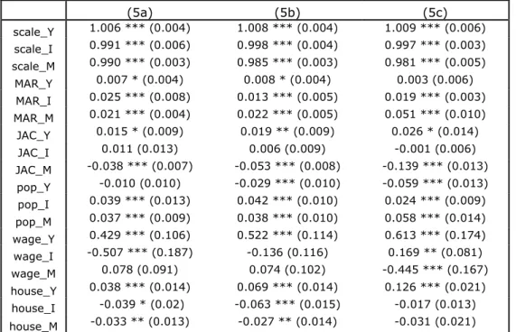
Obviously, the results above depend strongly on the definition of the industry stages. Therefore, we rerun model (5) for two alternative life cycle stage definitions. Column (5a) in table 8 shows the results when the category of intermediate industries is narrowed and the line demarcating mature and young industries becomes thinner. Column (5b) uses the same limits as in table 7, and in column (5c) the intermediate category is widened at the expense of the young and the mature categories.

If our hypotheses are correct, the parameter estimates of young and mature industries should lie closer together in column (5a) and further apart in column (5c). As we move from (5a) to (5b) to (5c), industries classified as mature become increasingly older and industries classified as young become increasingly younger.

Indeed, the patterns in both MAR and Jacobs’ externalities are amplified when moving from column (5a) to (5b) and then to (5c). The MAR externalities for mature industries rise steadily when the industries that are classified as mature become older, whereas the coefficients for young industries remain the same. The results concerning Jacobs’ externalities also get more extreme. For young industries, they get higher and higher when moving from left to right over the table, whereas for mature industries they become more negative.

The patterns in the variables that measure urbanization externalities get also more pronounced. For all variables – pop, house and wage, - the difference between the estimates for mature and young industries increases. In sum, table 8 strongly supports that the results in table 7 are robust and in line with our theoretical expectations.23

-Table 8 about here-

7: Conclusions

After more than two decades of investigating the importance of MAR, Jacobs’ and urbanization externalities, no consensus has arisen in the literature concerning the impacts of externalities on innovation and growth. Our conjecture at the beginning of the article was that industries have different agglomeration needs at different phases of their life cycle. In order to test this, we set up a framework that describes the evolution of agglomeration externalities along the life cycle of industries.

In terms of methodology, we use a procedure that solves some of the main issues encountered in empirical research in this field. For instance, the use of our city-potentials is a response to the Modifiable Areal Unit problem found in the literature. Another improvement can be found in the use of FEVD estimators to estimate the impact of population, which typically shows very little time-variation. Finally, we disentangled many of the different sources of urbanization externalities by using information on local house prices and wages.

In all, our results show that the benefits industries derive from their local environment are strongly associated with their stage in the industry life cycle. Moving from young, via intermediate to mature industries, the benefits derived from local specialization steadily

23

# - '

8

20 increase. In contrast, the benefits from local diversity for young industries are positive, then turn insignificant for intermediate industries and become negative for mature industries. These findings support our hypothesis that with increasing levels of maturity, industries experience rising benefits of intra-industry spillovers, whereas inter-industry spillovers decline in importance. The relative stability of these industries allows them to take advantage of local embeddedness. Therefore, additionally, mature industries are confronted with the problem of a lack of local focus in diversified cities that is absent for the less locally embedded and less standardized young industries. We also show that, in line with our ILC framework, factor costs and quality of labour have very different effects on the efficiency of young industries on the one hand, and mature industries on the other hand. Whereas the former thrive in expensive, medium sized cities with highly qualified and costly labour, the latter are better off in low cost cities with a relatively large local market.

The findings so far have many implications for the discussions on the importance of regional externalities in evolving industries, and there are still many avenues of further research to explore. One is to abandon the city-industry aggregates and conduct a plant level study of externalities. With improved plant panel data, we will be able to do so in the future. Another issue is to study the renewal dynamics of the industries more in detail with product level data. Such information could provide information about the exact structure of the trajectory industries go through and of the specific innovation processes taking place in plants. A third issue of importance is to investigate the impact of related variety on the growth of the different industries. With improved measures of technological relatedness (Neffke et al, 2008), such issues could be tackled with greater exactness than has been done so far.

In sum, the results of this study show that it is possible to go beyond the static low tech/high tech dichotomy sometimes used to explain differences in the impacts of externalities between industries. Equally important, our conclusions call into question econometric studies that have treated agglomeration externalities for a specific industry to be fixed over time. This is clearly not the case, as we have demonstrated. Rather, the study of agglomeration externalities demands a dynamic, long-term perspective.

21 References

Abernathy, W J, and K B Clark. 1985. Innovation: Mapping the Winds of Creative Destruction. Research Policy 14:3-22.

Amin, A. (2003). Industrial districts. In A Companion to Economic Geography, edited by E Sheppard and T J Barnes. Oxford: Blackwell.

Arellano, M. (2003). Panel Data Econometrics. Oxford: Oxford University Press.

Asheim, B T. 2000. Industrial Districts: the Contributions of Marshall and Beyond. In The Oxford Handbook of Economic Geography, edited by G L Clark, M P Feldman and M S Gertler. Oxford: Oxford University Press.

Audretsch, D B, and M P Feldman. 1996. Innovative Clusters and the Industry Life Cycle. Review of Industrial Organization 11:253-273.

Bailey, T C, and A C Gatrell. 1995. Interactive spatial analysis. Harlow: Longman.

Boschma R A 1997 New Industries and Windows of Locational Opportunity. A Long-Term Analysis of Belgium, Erkunde 51: 12-22.

Combes P-P. 2000. Economic Structure and Local Growth: France, 1984-1993. Journal of Urban Economics 47: 329-355.

Combes, P-P, T Magnac, and J-M Robin. 2004. The dynamics of local employment in France. Journal of Urban Economics 56: 217-243.

Davelaar E J 1989, Incubation and Innovation. A Spatial Perspective, Amsterdam: VU.

Dixit, A.K. and Stiglitz, J.E. 1977. Monopolistic competition and optimum product diversity. The American Economic Review 67 (3): 297-308.

Duranton, G, and D Puga. 2001. Nursery Cities: Urban Diversity, Process Innovation, and the Life Cycle of Products. The American Economic Review 91 (5):1454-1477.

Duranton, G, and D Puga. 2004. Micro-foundation of urban agglomeration economies. In Handbook of Urban and Regional Economics, vol 4, edited by J. Henderson and J.-F. Thisse. Amsterdam: North-Holland.

Feldman, M P. 2000. Location and Innovation: the New economic Geography of Innovation, Spillovers, and Agglomeration. In The Oxford Handbook of Economic Geography, edited by G L Clark, M P Feldman and M S Gertler. Oxford: Oxford University Press.

Florida, R L. (2002). The rise of the creative class : and how it's transforming work, leisure, community and everyday life. New York: Basic Books.

Glaeser, E L. 2000. The new economics of urban and regional growth. In The Oxford Handbook of Economic Geography, edited by G L Clark, M P Feldman and M S Gertler. Oxford: Oxford University Press.

22 Glaeser, E L, H D Kallal, J A Scheinkman, and A Schleifer. 1992. Growth in Cities. The Journal of Political Economy 100 (6):1126-1152.

Glaeser, E L, and D C Maré. 2001. Cities and Skills. Journal of Labor Economics, 19, 2: 316-342.

Gort, M, and S Klepper. 1982. Time Paths in the Diffusion of Product Innovations. The Economic Journal 92 (367):630-653.

Grabher, G. (1993). The Weakness of Strong Ties: the Lock-in of Regional Development in the Ruhr Area. In The Embedded Firm. On the Socioeconomics of Interfirm Relations, edited by G Grabher. London and New Yor