Daily crude oil price forecasting using hybridizing wavelet and artificial neural network model

(1)

Research Article

Daily Crude Oil Price Forecasting Using Hybridizing Wavelet

and Artificial Neural Network Model

Ani Shabri

1

and Ruhaidah Samsudin

2

1_{Department of Science Mathematic, Faculty of Science, Universiti Teknologi Malaysia, 81310 Skudai, Johor, Malaysia}

2_{Department of Software Engineering, Faculty of Computing, Universiti Teknologi Malaysia (UTM), 81310 Skudai, Johor, Malaysia} Correspondence should be addressed to Ani Shabri; ani [email protected]

Received 24 January 2014; Revised 2 July 2014; Accepted 2 July 2014; Published 16 July 2014 Academic Editor: Marek Lefik

Copyright © 2014 A. Shabri and R. Samsudin. This is an open access article distributed under the Creative Commons Attribution License, which permits unrestricted use, distribution, and reproduction in any medium, provided the original work is properly cited.

A new method based on integrating discrete wavelet transform and artificial neural networks (WANN) model for daily crude oil price forecasting is proposed. The discrete Mallat wavelet transform is used to decompose the crude price series into one approximation series and some details series (DS). The new series obtained by adding the effective one approximation series and DS component is then used as input into the ANN model to forecast crude oil price. The relative performance of WANN model was compared to regular ANN model for crude oil forecasting at lead times of 1 day for two main crude oil price series, West Texas Intermediate (WTI) and Brent crude oil spot prices. In both cases, WANN model was found to provide more accurate crude oil prices forecasts than individual ANN model.

1. Introduction

Crude oil prices fluctuations are of significant interest to both financial practitioners and market participants. However, crude oil price is one of the most complex and difficult to model because fluctuation of the crude oil price is rather irregular, nonlinear, nonstationary, and with high volatility. Thus, accurate forecasting of the crude oil price time series is one of the greatest challenges and among the most important issues facing energy economists towards better decisions in several managerial levels. For this reason, many researchers have devoted considerable effort to the development of different types of models for crude oil price forecasting.

The application of the classical time series models such as autoregressive moving average (ARMA) model (Moham-madi and Su [1], Ahmad [2], Wang et al. [3], and Xie et al. [4]) and generalized autoregressive conditional heteroscedastic (GARCH) type models (Morana [5], Sadorsky [6], and Agnolucci [7]) for crude oil price forecasting has received much attention in the last decade. However, the above models can provide good prediction results, when the price series under study is basically linear or near linear, and have

a limited ability to capture nonlinearity and nonstationary in crude oil prices data.

Artificial neural network (ANN) techniques have shown great ability in modeling and forecasting nonlinear and complex time series. ANN offers an effective approach for handling large amounts of dynamic, nonlinear, and noise data. Numerous papers have already presented successful application of ANN for modeling and forecasting the crude oil price series (Lackes et al. [8], Khazem and Mazouz [9], Mirmirani and Li [10], Kulkarni and Haidar [11], Yu et al. [12], and Hu et al. [13]) as well as for forecasting real world time series. Their experimental results show that the performance of ANN is superior to various traditional statistical models. ANN has an ability to learn complex and nonlinear time series that is difficult to model with conventional models. However, there are some disadvantages of ANN. Although ANN has advantages of accurate forecasting, their perfor-mance in some specific situation is inconsistent (Khashei and Bijari [14]). ANN also often suffers from local minima and overfitting, and the network structure of this model is difficult to determine and it is usually determined by using a trial-and-error approach (Kis¸i [15]). In addition, ANN model has

Volume 2014, Article ID 201402, 10 pages http://dx.doi.org/10.1155/2014/201402

(2)

a limitation with nonstationary data and may not be able to handle nonstationary data if preprocessing of the input data is not done (Adamowski and Sun [16]).

In the last decade, wavelet transforms have been inves-tigated in diverse fields, such as in economics [18]; business [19], and hydrology [20]. Wavelet transforms have gained very high attention and have been found to be very effective with nonstationary time series data. Recently, different hybrid models based on wavelet transform have been improved in the field of oil price forecasting. For example, Qunli et al. [21] proposed a hybrid model based on wavelet transform and radial basis function (RBF) neural network to forecast the future oil price. They found that wavelet decomposes the original price sequence successfully as the input layer of the network RBF neural network model. Bao et al. [22] developed a hybrid model integrating wavelet and least squares support vector machines (LSSVM) for crude oil forecasting. Youesfi et al. [23] apply a wavelet methodology to decompose the crude oil price and extended them directly to make forecasts. de Souza e Silva et al. [24] apply wavelet analysis to omit high frequency noises and then use hidden Markov model to predict future price movement. He et al. [25] proposed a wavelet decomposed ensemble model to incorporate the Heterogeneous Market Hypothesis into the modeling process. However, in the crude oil field, a hybrid wavelet and ANN model have received very little attention and there are only a few applications of this model to forecast crude oil price series. Shambora and Rossitier [26] developed a hybrid wavelet and ANN model in crude oil forecasting. Jammazi and Aloui [27] explored the Haar A Trous wavelet and backpropagation neural network algorithm to develop a crude oil price forecasting model. Mingming and Jinliang [28] constructed a multiple wavelet recurrent neural network simulation model to analyze crude oil prices. Wavelet analysis was used to catch multiscale data characteristics, and recur-rent neural network model was used to simulate crude oil prices. The simulation results showed that the model has high prediction accuracy.

The main contribution of this paper is to propose a novel hybrid integrating wavelet transform and ANN model for crude oil forecasting. In order to catch this purpose, the daily West Texas Intermediate (WTI) and Brent crude oil spot price were decomposed into subseries at different scale by Mallat algorithm. Then, effective subseries were summed together and then used as inputs into the ANN model for crude oil forecasting. Finally to evaluate the model ability, the proposed model was compared with individual ANN model.

2. Artificial Neural Network

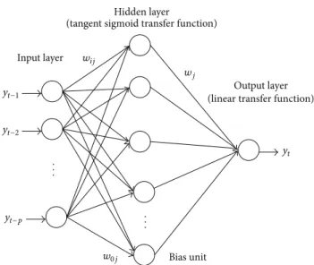
An ANN is flexible computing that has been extensively studied and used for time series forecasting in many areas of science and engineering since the early 1990s. ANN is a mathematical model which has a highly connected structure similar to brain cells. An ANN model usually consists of three layers: the first layer is the input layer where the data are introduced to the network, the second layer is the hidden layer where data are processed, and the last layer is the output

Input layer

Hidden layer

Output layer

Bias unit (tangent sigmoid transfer function)

(linear transfer function) yt−1 yt−2 yt−p w0j wj wij yt . . . . . .

Figure 1: Three-layer feedforward ANN model.

layer where the results of given input are produced.Figure 1

illustrates the architecture of the proposed ANN for crude

oil price forecasting. The relationship between the output(𝑦_𝑡)

and the input(𝑦_𝑡−1, 𝑦_𝑡−2, . . . , 𝑦_𝑡−𝑝)is given by [29]

𝑦_𝑡= 𝑏₀+∑𝑞 𝑗=1 𝑏_𝑗𝑓 (𝑤_0𝑗+∑𝑝 𝑖=1 𝑤_𝑖𝑗𝑦_𝑡−𝑖) + 𝜀_𝑡, (1) where𝑏_𝑗 (𝑗 = 0, 1, 2, . . . , 𝑞) and𝑤_𝑖𝑗(𝑖 = 0, 1, 2, . . . , 𝑝;𝑗 =

0, 1, 2, . . . , 𝑞) are the model parameters,𝑝is the number of

input nodes,𝑞is the number of hidden nodes, and𝑓(⋅)is the

transfer function.

Generally, ANN may have different transfer functions for different neurons in the same or different layers. The majority of research uses hyperbolic tangent sigmoid func-tion for hidden neurons and there is no consensus on which transfer function should be used for output neurons [30]. The hyperbolic tangent sigmoid is often used as the hidden layer transfer function, given by

𝑓 (𝑠) = 𝑒_𝑒𝑠_𝑠− 𝑒_{+ 𝑒}−𝑠_−𝑠 (2)

and one unit output layer is a pure linear transfer function, given by

𝑓 (𝑠󸀠) = 𝑠󸀠, (3)

where 𝑠 is the weighted input of the hidden layer, 𝑓(𝑠)

is hyperbolic tangent sigmoid transfer function for hidden

layer,𝑠󸀠is the weighted input of the output layer,𝑓(𝑠)is pure

linear transfer function for output layer.

The most popular neural network training method used is the backpropagation (BP) algorithm which is essentially a gradient steepest descent method introduced by Rumelhart et al. [31]. This algorithm suffers the problems of slow conver-gence, inefficiency, and lack of robustness [32]. Furthermore, it can be very sensitive to the choice of the learning rate. It is

(3)

hard to choose a proper learning rate, because a low-learning rate may result in long training times, and a high learning rate may cause system instability [33].

To overcome the weakness of BP algorithm, many researchers have investigated the use of Levenberg-Marquardt (LM) algorithm. The LM algorithm is one of the most popular and more efficient nonlinear optimisation methods. It is a variation of Newton’s method using Hessian-based algorithm for nonlinear least squares optimization which is used in most optimisation packages. The LM algorithm takes large steps down the gradient where the gradient is small, such as near local minima, and takes small steps when the gradient is large. Its faster convergence, robustness, and the ability to find good local minima make it attractive in ANN training. This optimisation technique is more powerful than the conventional gradient descent technique [34–36].

3. Wavelet Transform

The wavelet transforms is a strong mathematical tool that pro-vides a time-frequency representation of an analyzed signal in the time domin. This overcomes the basic shortcoming of Fourier analysis, which is that the Fourier spectrum contains only globally averaged information. Wavelet transformations provide useful decomposition of the original time series by capturing useful information on various decomposition levels. Wavelet transform can be divided by two categories: continuous wavelet transforms (CWT) and discrete wavelet

transforms (DWT). The CWT of the time series𝑥(𝑡)is given

by 𝑊 (𝜏, 𝑠) = 1 √|𝑠|∫ ∞ −∞𝑥 (𝑡) 𝜓 ∗ ( 𝑡 − 𝜏 𝑠 ) 𝑑𝑡, (4)

where (∗) indicates the conjugate complex function,𝑡stands

for a time, 𝜏 stands for the time step, 𝑠 ∈ [0, ∞] stands

for the wavelet scale, and𝜓(𝑡)is the transforming function

and is called the mother wavelet. The term wavelet means small wave, where small refers to the condition that the function is of a finite length. The wave refers to the condition that the function is of a finite length. Several families of

wavelets (𝜓) that have been proven to be useful for various

applications are described in related references (Mallat [37]). The wavelets are chosen based on their shape and their ability to analyse the time series in a particular application. Typical wavelet families such as Haar, Daubechies, Coiflet, Symlet, Meyer, Morlet, and the Mexican Hat can be used as a mother wavelet. The CWT is not often used for forecasting due to its computationally complex and time requirements to compute [38]. Instead, successive wavelet is often discrete in forecasting applications to simplify the numeric solutions. DWT requires less computation time and is simpler to apply. DWT is given by 𝜓_𝑚,𝑛(𝑡 − 𝜏_𝑠 ) = 1 √𝑠𝑚/2 0 𝜓 (𝑡 − 𝑛𝜏_𝑠_𝑚0𝑠𝑚0 0 ) , (5)

where𝑚and𝑛are integers that control the scale and time.

The most common and simplest choice for parameters are

𝑠₀ = 2 and 𝜏= 1. For a discrete time series𝑥(𝑡), the DWT

becomes

𝑊_{𝑚, 𝑛}= 2−𝑚/2𝑁−1_∑ 𝑡=0

𝜓 (2−𝑚_{𝑡 − 𝑛) 𝑥 (𝑡) ,} ₍₆₎

where𝑊_{𝑚, 𝑛}is the wavelet coefficient for the discrete wavelet

at scale𝑠 = 2𝑚and𝜏 = 2𝑚𝑛. According to the Mallat’s theory,

the original discrete time series𝑥(𝑡)can be decomposed into

a series of linearly independent approximation and detail signals by using the inverse DWT. The inverse DWT is given by 𝑥 (𝑡) = 𝑇 + ∑𝑀 𝑚=1 2𝑀−𝑚−1 ∑ 𝑡=0 𝑊_𝑚,𝑛2−𝑚/2𝜓 (2−𝑚𝑡 − 𝑛) (7) or in a simple format as 𝑥 (𝑡) = 𝐴𝑀(𝑡) + 𝑀 ∑ 𝑚=1 𝐷_𝑚(𝑡) (8)

in which𝐴_𝑀(𝑡)is called approximation subseries or residual

term at levels 𝑀 and 𝐷_𝑚(𝑡)(𝑚 = 1, 2, . . . , 𝑀) is detailed

subseries which can capture small features of interpretational value in the data.

4. Application

In this study, two main crude oil prices, Brent crude oil spot price and West Texas Intermediate (WTI) crude oil spot price (in US dollars per barrel) series, were chosen as the experimental sample. The main reason for selecting these crude oil spot price indicators is that these two crude oil prices are the most famous benchmark prices, which are widely used as the basis of many crude oil price formulae

[12,17]. For Brent data, we use the daily data from May 20,

1987, to September 30, 2006, with a total of 4933 observations. Data from May 20, 1987, to December 31, 2002, are used for the training set (3965 observations), and the remainder is used as the testing set (968 observations).

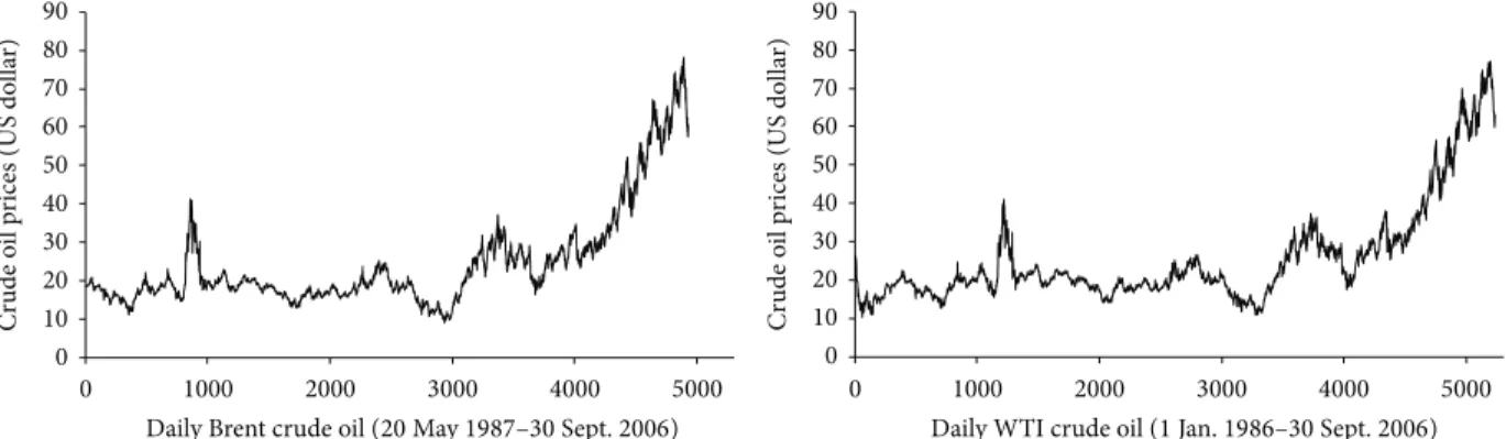
While, for WTI data, the daily data from January 1, 1986, to September 30, 2006, excluding public holidays, with a total of 5237 were employed as experimental data, for convenience of WANN modeling, the data from January 1, 1986, to December 31, 2000, are used for the training set (3800 observations), and the remainder is used as the testing set (1437 observations). The graphical representation of the price

for Brent and WTI crude oil price is given inFigure 2.

In practice, short-term forecasting results are more useful as they provide timely information for the correction of forecasting value. In this study, two performance criteria such as RMSE and MAPE were used to evaluate the accuracy of the models. These criteria are given below:

RMSE= √1 𝑛 𝑛 ∑ 𝑡=1 (𝑦_𝑡− ̂𝑦_𝑡)2, MAPE= 1 𝑛 𝑛 ∑ 𝑡=1 |BIAS| , (9)

(4)

0 10 20 30 40 50 60 70 80 90 0 1000 2000 3000 4000 5000 Cr ude o il p rices (US do lla r) 0 10 20 30 40 50 60 70 80 90 0 1000 2000 3000 4000 5000 Cr ude o il p rices (US do lla r)

Daily Brent crude oil (20May1987–30Sept.2006) Daily WTI crude oil (1Jan.1986–30Sept.2006)

Figure 2: Daily Brent and WTI crude oil prices series.

where BIAS = (𝑦_𝑡 − ̂𝑦_𝑡)/𝑦_𝑡, 𝑦_𝑡 is the actual and ̂𝑦_𝑡 is the

forecasted value of period𝑡, and𝑛is the number of total

observations. The criteria to judge for the best model are relatively small RMSE and MAPE found in the training and testing of the data.

5. Fitting ANN Model to the Data

At first, the multilayer perceptron (MLP) feedforward ANN model without any data preprocessing was used to model the crude oil price series. One of the most important steps in the model development process of the ANN model is the determination of significant input variables. There are no fixed rules for the selection of input variables for developing ANN model, even though a general framework can be followed based on previous successful application in crude oil prices problems [39]. For Brent and WTI data, six input combinations based on previous log return of daily oil prices are evaluated to estimate current prices value. The input

combinations evaluated in the study are (i)𝑦_𝑡−1, (ii)𝑦_𝑡−1,𝑦_𝑡−2,

(iii)𝑦_𝑡−1,𝑦_𝑡−2,𝑦_𝑡−3, (iv) 𝑦_𝑡−1,𝑦_𝑡−2,𝑦_𝑡−3,𝑦_𝑡−4, (v)𝑦_𝑡−1, 𝑦_𝑡−2,

𝑦_𝑡−3,𝑦_𝑡−4,𝑦_𝑡−5, and (vi)𝑦_𝑡−1,𝑦_𝑡−2,𝑦_𝑡−3,𝑦_𝑡−4,𝑦_𝑡−5,𝑦_𝑡−6.

ANN model used in this study is the standard three-layer feedforward network. For improving the network modeling and reducing the chance of being trapped in a local minima, data normalization is applied in ANN input and output. Due to the crude oil prices series for both data collected are

nonstationary (seeFigure 2); to improve the accuracy of the

training and testing, each data point in the input neurons had to be preprocessed by normalizing and transformed

within the range of [−1, 1]. There are no fixed rules as to

which standardization approach should be used in particular circumstances. In this study, normalization for each raw input and output data set was calculated by taking log return of current oil prices as the following formula:

𝑅_𝑡=log( 𝑦𝑡

𝑦_𝑡−1) , (10)

where𝑦_𝑡and𝑦_𝑡−1are current and one-period lagged prices.

To achieve optimal weights of ANN, LM algorithm pro-vided by the MATLAB neural network toolbox is used to train the network. In this study, the hyperbolic tangent sigmoid

function and a linear function are employed as activation functions for the hidden and output layers, respectively. The initial value of learning rate is set to 0.001 and a momentum coefficient of 0.9. The learning rate is increased by a factor of 10 and a decrease step of 0.1 until the change above results in a reduced performance value. The number of epochs that are used to train is set to 1000. The training of ANN will stop

when the error achieves 10−5or when the number of epochs

reaches 1000.

The hidden layer plays important roles in many successful applications of ANN. It has been proven that only one hidden layer is sufficient for ANN to approximate any complex nonlinear function with any desired accuracy. In the case of the popular one hidden layer networks, several practical numbers of neurons in the hidden layer were identified for better forecasting accuracy. The optimal number of nodes in the hidden layer was identified using several practical guidelines. Berry and Linoff [40] claimed that the number

of hidden nodes should never be more than 2𝐼, where𝐼 is

the number of inputs. Hecht-Nielsen [41] claimed that the

number of hidden neuron is equal to 2𝐼+ 1. However, as far as

the number of hidden neurons is concerned, there is currently no theory to determine how many nodes in the hidden layer are optimal. In the present study, the number of hidden nodes

was progressively increased from 1 to 2𝐼+ 1.

A program code including the wavelet toolbox was written in MATLAB language for the development of the ANN model. The optimal complexity of ANN model, that is, the number of input and hidden nodes, was determined by a

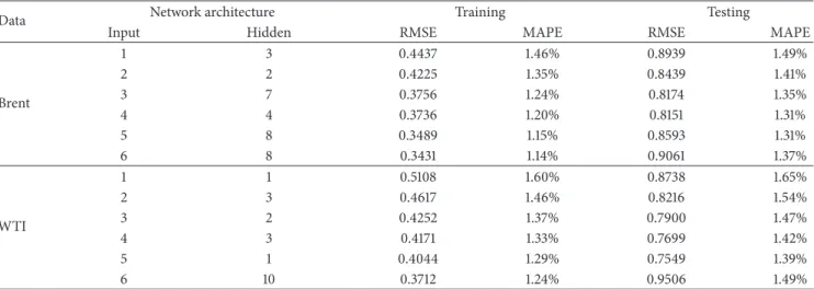
trial-and-error approach.Table 1shows the best performance

results of different ANN with different numbers of hidden

neurons from 1 to 2𝐼 + 1 for both data series. The training

set is used to estimate parameters for any specific ANN architecture. The testing set is then used to select the best ANN among all numbers of hidden neurons considered.

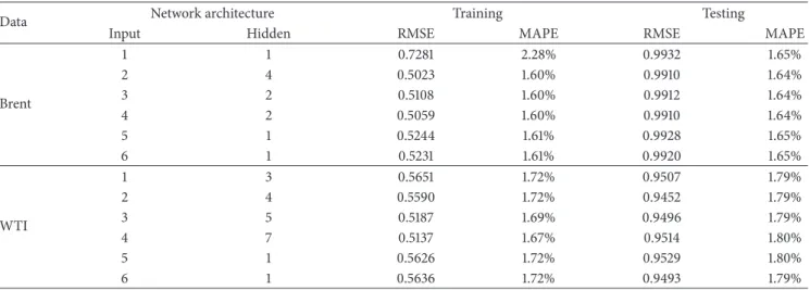
Table 1shows the performance of ANN varying in

accor-dance with the number of neurons in the hidden layer. It can be seen that the prediction errors (%MAPE) by ANN range from 1.60% to 2.28% for Brent data and from 1.67% to 1.80% for WTI data. For Brent data, the best architecture according RMSE and MAPE criterion for training data and testing data has 2 input layer neurons, 4 hidden layer neurons, and 1 output layer neuron (2-4-1). For this architecture, RMSE

(5)

Table 1: Training and testing performance of different network architecture of ANN model.

Data Network architecture Training Testing

Input Hidden RMSE MAPE RMSE MAPE

Brent 1 1 0.7281 2.28% 0.9932 1.65% 2 4 0.5023 1.60% 0.9910 1.64% 3 2 0.5108 1.60% 0.9912 1.64% 4 2 0.5059 1.60% 0.9910 1.64% 5 1 0.5244 1.61% 0.9928 1.65% 6 1 0.5231 1.61% 0.9920 1.65% WTI 1 3 0.5651 1.72% 0.9507 1.79% 2 4 0.5590 1.72% 0.9452 1.79% 3 5 0.5187 1.69% 0.9496 1.79% 4 7 0.5137 1.67% 0.9514 1.80% 5 1 0.5626 1.72% 0.9529 1.80% 6 1 0.5636 1.72% 0.9493 1.79%

Table 2: Coefficient of determination (𝑅2) between each of subtime series for Brent and WTI data.

Data DWT Coefficient of determination (𝑅

2_{) with original crude oil prices series} _Mean

𝑡 − 1 𝑡 − 2 𝑡 − 3 𝑡 − 4 𝑡 − 5 𝑡 − 6 𝑅2 Brent D1 0.0000 0.0000 0.0000 0.0000 0.0000 0.0000 0.0000 D2 0.0000 0.0000 0.0001 0.0002 0.0000 0.0000 0.0001 D3 0.0006 0.0006 0.0002 0.0000 0.0002 0.0002 0.0003 A3 0.9895 0.9917 0.9937 0.9954 0.9967 0.9967 0.9940 WTI D1 0.0000 0.0052 0.0021 0.0053 0.0000 0.1619 0.0291 D2 0.0027 0.0149 0.0001 0.0866 0.1092 0.0274 0.0402 D3 0.0353 0.0622 0.0472 0.0060 0.0107 0.0750 0.0394 A3 0.0040 0.0143 0.0311 0.0511 0.0721 0.0886 0.0435

value is 0.9910 and MAPE value is 1.64% for testing data, while, for WTI data, the best architecture according to RMSE (0.9452) and MAPE (1.79%) criterion for testing data is 2-4-1.

6. Fitting Hybrid Wavelet-ANN

Model to the Data

The hybrid wavelet and ANN (WANN) model is obtained by combining two methods, discrete wavelet transform (DWT) and ANN model. In WANN, the original crude oil price series was decomposed into a certain number of subtime series components which were entered to ANN in order to improve the model accuracy. In this study, the Daubechies wavelet, one of the most widely used wavelet families, is chosen as the wavelet function to decompose the original series (Eynard et al. [42]; Bagheri et al. [43]). When conducting wavelet analysis, the number of decomposition levels that are appropriate for the data must be chosen. To choose the number of decomposition level, the following formula is used [34]:

𝐿 =int[log(𝑁)] , (11)

where𝐿is the level of decomposition and𝑁is the number

of time series data. According to this formula, the optimal number of decomposition levels for both crude oil price

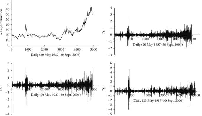
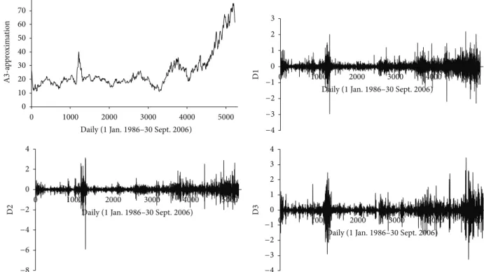
series data in this study would have been 3. For this purpose, firstly, the original oil price series is decomposed into 3 level components (D1, D2, and D3) that stand for different frequency components of the original series (details) and an

approximation component (A3), as shown in Figures3and4.

Each of D’s series plays a distinct role in the original time series and has different effects on the original crude price series. Instead of using each D’s component individually as model input, employment of the added suitable D’s compo-nent is more useful and can highly increase forecast per-formances of hybrid models. In this study, the effectiveness of wavelet components is determined using the coefficient

of determination (R2) between each D’s subtime series and

original data. TheR2values are given inTable 2. It can be seen

thatR2of the D1 is zero for Brent data and 0.0291 for WTI

data. However, the wavelet components D2 and D3 show

significantly higherR2 compared to the D1 for both series.

According to theR2 analyses, the effective components D2

and D3 were selected as the dominant wavelet components. Afterward, the significant wavelet components D2, D3 and approximation (A3) component were added to each other as

ANN model input for crude oil forecast.Figure 6shows the

structure of the WANN model.Figure 5shows the original

crude oil prices and their Ds, that is, the time series of 2-month mode (D1), 4-2-month mode (D2), 8-2-month mode (D3),

(6)

0 10 20 30 40 50 60 70 80 90 0 1000 2000 3000 4000 5000 A 3 -a p p ro xima tio n −3 −2 −1 0 1 2 3 4 0 1000 2000 3000 4000 5000 D 1 −4 −3 −2 −1 0 1 2 3 0 1000 2000 3000 4000 5000 D 2 −5 −4 −3 −2 −10 1 2 3 4 5 6 0 1000 2000 3000 4000 5000 D 3

Daily (20May1987–30Sept.2006)

Figure 3: Decomposed wavelet subtime series components (Ds) and approximation (As) of Brent crude oil.

approximate mode (A3), and the combinations of effective details and approximation components mode (DW = A2 + D2 + D3).

Six different combinations of the new series input data are used in this study. WANN model was trained in the same way as the ANN model, with the exception that the inputs were the combinations of effective details and approximation components mode (DW) after the appropriate wavelet decomposition was selected. The input combinations for WANN model evaluated in the study are

(i) DW_𝑡−1, (ii) DW_𝑡−1, DW_𝑡−2, (iii) DW_𝑡−1, DW_𝑡−2, DW_𝑡−3, (iv) DW_𝑡−1, DW_𝑡−2, DW_𝑡−3, DW_𝑡−4, (v) DW_𝑡−1, DW_𝑡−2, DW_𝑡−3, DW_𝑡−4, DW_𝑡−5and (vi) DW_𝑡−1, DW_𝑡−2, DW_𝑡−3, DW_𝑡−4, DW_𝑡−5, DW_𝑡−6.

In all cases, the input and output are transformed into the log return of current oil prices. The selection of the optimal number of nodes in both the input and hidden layers was done in the same way as for the ANN model. The model architecture for WANN consists of 1 to 6 nodes in the input

layer (𝐼), 1 to 2𝐼+ 1 nodes in the hidden layer, and one neuron

in the output layer. The data was partitioned into training and testing sets in the same manner as the ANN model.

The performance measures of WANN for both crude oil

data are shown in Table 3. According to Table 3, the best

architecture of ANN according to RMSE and MAPE criterion is 4-4-1 for Brent data and 5-1-1 for WTI data.

For further analysis, the best performances are compared for the ANN and WANN models in terms of the RMSE and MAPE in the testing phase. The statistical results of different

models are summarized inTable 4.

For Brent data, WANN improved ANN forecast about 17.7% and 20.1% reduction in RMSE and MAPE values, respectively. For WTI data, WANN obtained the best value of RMSE and MAPE during the testing phase which decreases by 20.1% and 22.3%, respectively, comparing with ANN. Generally, it can be observed that WANN model outperforms ANN for both data. Thus, the results indicate that WANN is able to obtain the best result in terms of different evaluation measures during the testing phase.

In order to further compare in terms of forecasting accuracy, Diebold-Mariano (DM) test statistic is used to test the statistical significance of different forecasting models [44]. DM statistic can be defined as

DM= 𝑑

√𝑉_𝑑/𝐹, (12)

where𝑑_𝑡 = ∑𝐹_𝑡=1(𝑦_𝑡− ̂𝑦WANN,𝑡)2− ∑𝐹𝑡=1(𝑦𝑡− ̂𝑦ANN,𝑡)2,𝑑 =

(∑𝐹_𝑡=1𝑑_𝑡)/𝐹, 𝑉_𝑑 = 𝛾₀ + 2 ∑_𝑙=1∞ 𝛾_𝑙, and 𝛾_𝑙 = cov(𝑑_𝑡, 𝑑_𝑡−𝑙).

̂𝑦ANN,𝑡and̂𝑦WANN,𝑡are forecast values from ANN and WANN

models, respectively. The null hypothesis of equal forecast accuracy is rejected if the test statistic is negative and

statistically significant.Table 4reports the estimate values of

DM test statistic for testing performance of WANN compared

with ANN.Table 4shows that all DM values of the proposed

WANN for Brent and WTI data are below −2.326 and

(7)

0 10 20 30 40 50 60 70 80 0 1000 2000 3000 4000 5000 A 3 -a p p ro xima tio n −4 −3 −2 −1 0 1 2 3 0 1000 2000 3000 4000 5000 D 1 −8 −6 −4 −2 0 2 4 0 1000 2000 3000 4000 5000 D 2 −4 −3 −2 −1 0 1 2 3 4 0 1000 2000 3000 4000 5000 D 3

Daily (1Jan.1986–30Sept.2006)

Daily (1Jan.1986–30Sept.2006) Daily (1Jan.1986–30Sept.2006)

Figure 4: Decomposed wavelet subtime series components (Ds) and approximation (As) of WTI crude oil.

Data collection (y_t)

Input time series

yt= f(yt−1, yt−2, . . . , yt−p) Decompose input using DWT yt−1 yt−2 yt−p · · · Add the effects of Ds A3t−1 A3t−2 A3t−p The effectiveness of DWT as input for ANN D1_t−1 D2_t−1 D3_t−3

DW_t−1 DWt−2 DW_t−p

D1_t−2 D2_t−2 D3_t−2 D1t−p D2t−p D3_t−p

yt= f(DW_t−1,DW_t−2, . . . ,DW_t−p) Figure 5: The structure of the WANN model.

the proposed model performs the best in forecasting oil price in short term at least at the 99% confidence level. Now, DM test statistic provides stronger support for WANN model.

Figure 6shows the box plots of the BIAS values computed

using ANN and WANN for Brent and WTI data. The picture produced consists of the most extreme values in the data set, the lower and upper quartiles, and the median. The criterion

for selecting a suitable model is based on the minimum achieved by median BIAS value and dispersion in BIAS.

Figure 6shows that the performance of WANN is better than

the ANN for Brent and WTI data.

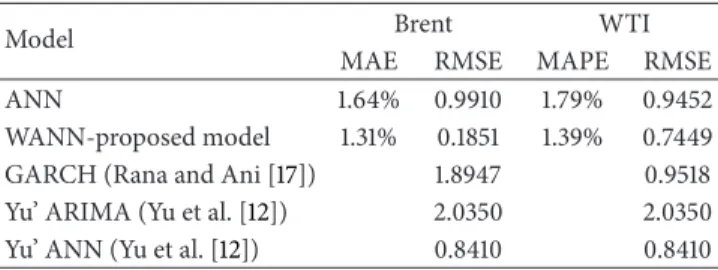
Finally, in order to evaluate the efficiency of the proposed hybrid model, the obtained results were also compared with the results of ANN and ARIMA [12] and GARCH [17] models

(8)

WANN ANN 0.10 0.05 0.00 −0.05 −0.10 −0.15 −0.20 Bi as ( % )

WTI crude oil prices

WANN ANN 0.10 0.05 0.00 −0.05 −0.10 −0.15 Bi as ( % )

Brent crude oil prices

Figure 6: Comparison of ANN and WANN models for the testing results.

Table 3: Training and testing performance of different network architecture of WANN model.

Data Network architecture Training Testing

Input Hidden RMSE MAPE RMSE MAPE

Brent 1 3 0.4437 1.46% 0.8939 1.49% 2 2 0.4225 1.35% 0.8439 1.41% 3 7 0.3756 1.24% 0.8174 1.35% 4 4 0.3736 1.20% 0.8151 1.31% 5 8 0.3489 1.15% 0.8593 1.31% 6 8 0.3431 1.14% 0.9061 1.37% WTI 1 1 0.5108 1.60% 0.8738 1.65% 2 3 0.4617 1.46% 0.8216 1.54% 3 2 0.4252 1.37% 0.7900 1.47% 4 3 0.4171 1.33% 0.7699 1.42% 5 1 0.4044 1.29% 0.7549 1.39% 6 10 0.3712 1.24% 0.9506 1.49%

Table 4: Forecasting performance indices of ANN and WANN.

Data ANN WANN DM

RMSE MAPE RMSE MAPE WANN versus ANN

Brent 0.9910 1.64% 0.8151 1.31% −4.0416∗ WTI 0.9452 1.79% 0.7549 1.39% −9.3756∗

∗_{Significant at 1% level.}

using the same data. The comparison has been summarized in

Table 5. The results are tabulated inTable 5in which the linear

ARIMA and GARCH models were unable to completely model the complex nonlinearity and high irregularity of the crude oil prices. However, when ANN is used, the model could capture both nonlinear and complex features of the crude oil price series. ANN model performs much better than the ARIMA and GARCH models which demonstrate the existence and importance of nonlinear and nonstationary behavior in the crude oil price time series. However, ANN model is less efficient compared to proposed WANN model. It is observed that the proposed model yields better result than the other models for both crude oil price data. This result shows that the new input series from discrete wavelet

transforms have significant extremely positive effect on ANN model results.

7. Conclusions

In this study the wavelet transform and the ANN model were combined in order to develop a hybrid model for modeling and forecasting the crude oil price series. In the first model, ANN model without any data preprocessing was used to model the crude oil price series. In the second proposed hybrid model, the wavelet transform can capture the multi-scale features of a time series, which was used to decompose the crude oil price series. In this study, the new series obtained by adding the effective wavelet components was used as input to the ANN model to forecast the crude oil price at one time step ahead. It is recommended that the sum of effective details and the approximation component in modeling by ANN should be selected rather than using all subtime series components. Effective wavelet components are selected based on correlation between particular component series (approximation series and some details series) and crude oil price series. The performance of the proposed WANN model was compared to ANN model. The hybrid model showed

(9)

Table 5: The RMSE and MAPE comparisons for different models.

Model Brent WTI

MAE RMSE MAPE RMSE

ANN 1.64% 0.9910 1.79% 0.9452

WANN-proposed model 1.31% 0.1851 1.39% 0.7449

GARCH (Rana and Ani [17]) 1.8947 0.9518

Yu’ ARIMA (Yu et al. [12]) 2.0350 2.0350

Yu’ ANN (Yu et al. [12]) 0.8410 0.8410

a great improvement in crude oil price modeling and pro-duced better forecasts than ANN model alone. The study concludes that the forecasting abilities of WANN model are found to be improved when the wavelet transformation tech-nique is adopted for the data preprocessing. The decomposed periodic components obtained from DWT technique are found to be most effective in yielding accurate forecast when used as inputs in ANN model. The accurate forecasting results indicate that WANN model provides a superior alternative to other models and a potentially very useful new method for crude oil price forecasting.

Conflict of Interests

The authors declare that there is no conflict of interests regarding the publication of this paper.

Acknowledgments

The authors would like to thank the Universiti Teknologi Malaysia and Ministry Of Science, Technology and Inno-vation (MOSTI) for providing research funding (Grant no. 4F399) to support this piece of research.

References

[1] H. Mohammadi and L. Su, “International evidence on crude oil price dynamics: applications of ARIMA-GARCH models,” Energy Economics, vol. 32, no. 5, pp. 1001–1008, 2010.

[2] M. I. Ahmad, “Modelling and forecasting Oman Crude Oil Prices using Box-Jenkins techniques,”International Journal of Trade and Global Markets, vol. 5, pp. 24–30, 2012.

[3] S. Y. Wang, L. Yu, and K. K. Lai, “A novel hybrid AI system framework for crude oil price forecasting,”Lecture Notes in Computer Science, vol. 3327, pp. 233–242, 2004.

[4] W. Xie, L. Yu, S. Xu, and S. Wang, “A new method for crude oil price forecasting based on support Vector machines,” in Proceedings of the International Conference on Computational Science (Part IV), pp. 444–451, 2006.

[5] C. Morana, “A semiparametric approach to short-term oil price forecasting,”Energy Economics, vol. 23, no. 3, pp. 325–338, 2001. [6] P. Sadorsky, “Modeling and forecasting petroleum futures volatility,”Energy Economics, vol. 28, no. 4, pp. 467–488, 2006. [7] P. Agnolucci, “Volatility in crude oil futures: a comparison of

the predictive ability of GARCH and implied volatility models,” Energy Economics, vol. 31, no. 2, pp. 316–321, 2009.

[8] R. Lackes, C. B¨orgermann, and M. Dirkmorfeld, “Forecasting the price development of crude oil with artificial neural net-works,”Distributed Computing, Artificial Intelligence, Bioinfor-matics, Soft Computing, and Ambient Assisted Living, vol. 5518, pp. 248–255, 2009.

[9] H. Khazem and A. Mazouz, “Forecasting the price of crude oil using artificial neural networks,”International Journal of Business, Marketing, and Decision Sciences, vol. 6, no. 1, pp. 119– 135, 2013.

[10] S. Mirmirani and H. C. Li, “A comparison of VAR and neural networks with genetic algorithm in forecasting price of oil,” Advances in Econometrics, vol. 19, pp. 203–223, 2004.

[11] S. Kulkarni and I. Haidar, “Forecasting model for crude oil price and commodity futures prices using artificial neural networks,” International Journal of Computer Science & Information Secu-rity, vol. 2, no. 1, pp. 81–88, 2009.

[12] L. Yu, S. Wang, and K. K. Lai, “Forecasting crude oil price with an EMD-based neural network ensemble learning paradigm,” Energy Economics, vol. 30, no. 5, pp. 2623–2635, 2008. [13] J. W. Hu, Y. Hu, and R. R. Lin, “Applying neural networks to

prices prediction of crude oil futures,”Mathematical Problems in Engineering, vol. 2012, Article ID 959040, 12 pages, 2012. [14] M. Khashei and M. Bijari, “A novel hybridization of artificial

neural networks and ARIMA models for time series forecast-ing,”Applied Soft Computing Journal, vol. 11, no. 2, pp. 2664– 2675, 2011.

[15] ¨O. Kis¸i, “Neural network and wavelet conjunction model for modelling monthly level fluctuations in Turkey,”Hydrological Processes, vol. 23, no. 14, pp. 2081–2092, 2009.

[16] J. Adamowski and K. Sun, “Development of a coupled wavelet transform and neural network method for flow forecasting of non-perennial rivers in semi-arid watersheds,”Journal of Hydrology, vol. 390, no. 1-2, pp. 85–91, 2010.

[17] A. A. Rana and S. Ani, “Daily crude oil price forecasting model using arima, generalized autoregressive conditional het-eroscedastic and support vector machines,”American Journal of Applied Sciences, vol. 11, no. 3, pp. 425–432, 2014.

[18] P. Hajto, “A neural economic time series prediction with the use of a wavelet analysis,”Schedae Informaticae, vol. 11, pp. 115–132, 2002.

[19] W. Tong and Y. Li, “Wavelet method combining BP networks and time series ARMA modeling for data mining forecasting,” inAdvances in Natural Computation, vol. 3611 ofLecture Notes in Computer Science, pp. 123–134, Springer, New York, NY, USA, 2005.

[20] V. Nourani, M. Komasi, and A. Mano, “A multivariate ANN-wavelet approach for rainfall-runoff modeling,”Water Resources Management, vol. 23, no. 14, pp. 2877–2894, 2009.

[21] W. Qunli, H. Ge, and C. Xiaodong, “Crude oil price forecasting with an improved model based on wavelet transform and RBF neural network,” inProceeding of the International Forum on Information Technology and Applications, vol. 1, pp. 231–234, 2009.

[22] Y. Bao, X. Zhang, L. Yu, K. K. Lai, and S. Wang, “An model using wavelet decomposition squares support vector machines crude oil prices forecasting,”New Mathematics Computation, vol. 7, no. 299, pp. 299–311, 2011.

[23] S. Yousefi, I. Weinreich, and D. Reinarz, “Wavelet-based predic-tion of oil prices,”Chaos, Solitons and Fractals, vol. 25, no. 2, pp. 265–275, 2005.

(10)

[24] E. G. de Souza e Silva, L. F. L. Legey, and E. A. de Souza e Silva, “Forecasting oil price trends using wavelets and hidden Markov models,”Energy Economics, vol. 32, no. 6, pp. 1507–1519, 2010. [25] K. He, L. Yu, and K. K. Lai, “Crude oil price analysis and

fore-casting using wavelet decomposed ensemble model,”Energy, vol. 46, no. 1, pp. 564–574, 2012.

[26] W. E. Shambora and R. Rossiter, “Are there exploitable ineffi-ciencies in the futures market for oil?”Energy Economics, vol. 29, no. 1, pp. 18–27, 2007.

[27] R. Jammazi and C. Aloui, “Crude oil price forecasting: exper-imental evidence from wavelet decomposition and neural network modeling,”Energy Economics, vol. 34, no. 3, pp. 828– 841, 2012.

[28] T. Mingming and Z. Jinliang, “A multiple adaptive wavelet recurrent neural network model to analyze crude oil prices,” Journal of Economics and Business, vol. 64, no. 4, pp. 275–286, 2012.

[29] G. Zhang, B. Eddy Patuwo, and M. Y. Hu, “Forecasting with artificial neural networks: the state of the art,” International Journal of Forecasting, vol. 14, no. 1, pp. 35–62, 1998.

[30] P. Coulibaly and N. D. Evora, “Comparison of neural network methods for infilling missing daily weather records,”Journal of Hydrology, vol. 341, no. 1-2, pp. 27–41, 2007.

[31] D. E. Rumelhart, J. L. McClelland, and The PDP Research Group, Parallel Distributed Processing: Explorations in the Microstructure of Cognition, vol. 1-2, MIT Press, Cambridge, Mass, USA, 1986.

[32] G. Zhang, B. E. Patuwo, and M. Y. Hu, “Forecasting with artificial neural networks: the state of the art,” International Journal of Forecasting, vol. 14, no. 1, pp. 35–62, 1998.

[33] H. R. Maier and G. C. Dandy, “Neural networks for the prediction and forecasting of water resources variables: a review of modelling issues and applications,”Environmental Modelling and Software, vol. 15, no. 1, pp. 101–124, 2000.

[34] V. Nourani, M. T. Alami, and M. H. Aminfar, “A combined neural-wavelet model for prediction of Ligvanchai watershed precipitation,”Engineering Applications of Artificial Intelligence, vol. 22, no. 3, pp. 466–472, 2009.

[35] B. Khalil, T. B. M. J. Ouarda, and A. St-Hilaire, “Estimation of water quality characteristics at ungauged sites using artificial neural networks and canonical correlation analysis,”Journal of Hydrology, vol. 405, no. 3-4, pp. 277–287, 2011.

[36] J. P. S. Catal˜ao, H. M. I. Pousinho, and V. M. F. Mendes, “Short-term wind power forecasting in Portugal by neural networks and wavelet transform,”Renewable Energy, vol. 36, no. 4, pp. 1245–1251, 2011.

[37] S. G. Mallat, “Theory for multiresolution signal decomposition: the wavelet representation,”IEEE Transactions on Pattern Anal-ysis and Machine Intelligence, vol. 11, no. 7, pp. 674–693, 1989. [38] R. Gencay, F. Selcuk, and B. Whitcher, An Introduction to

Wavelets and Other Filtering Methods in Finance and Economics, Academic Press, San Diego, Calif, USA, 2002.

[39] I. Haidar, S. Kulkarni, and H. Pan, “Forecasting model for crude oil prices based on artificial neural networks,” inProceedings of the International Conference on Intelligent Sensors, Sensor Networks and Information Processing, pp. 103–108, 2008. [40] M. J. A. Berry and G. S. Linoff,Data Mining Techniques: For

Marketing, Sales, and Customer Support, John Wiley & Sons, New York, NY, USA, 1997.

[41] R. Hecht-Nielsen,Neurocomputing, Addison-Wesley, Reading, Mass, USA, 1990.

[42] J. Eynard, S. Grieu, and M. Polit, “Wavelet-based multi-resolution analysis and artificial neural networks for forecasting temperature and thermal power consumption,” Engineering Applications of Artificial Intelligence, vol. 24, no. 3, pp. 501–516, 2011.

[43] A. Bagheri, H. M. Peyhani, and M. Akbari, “Financial fore-casting using ANFIS networks with quantum-behaved particle swarm optimization,”Expert Systems with Applications, vol. 41, no. 14, pp. 6235–6250, 2014.

[44] F. X. Diebold and R. S. Mariano, “Comparing predictive accuracy,”Journal of Business and Economic Statistics, vol. 20, no. 1, pp. 134–144, 2002.

(11)

Submit your manuscripts at

http://www.hindawi.com

Hindawi Publishing Corporation

http://www.hindawi.com Volume 2014

Mathematics

Journal of

Mathematical Problems in Engineering

Hindawi Publishing Corporation http://www.hindawi.com

Differential Equations

International Journal of

Volume 2014 Hindawi Publishing Corporation

http://www.hindawi.com Volume 2014 Hindawi Publishing Corporationhttp://www.hindawi.com Volume 2014

Mathematical PhysicsAdvances in

Complex Analysis

Journal of

Optimization

Journal of

Combinatorics

Journal of

Function Spaces

Abstract and Applied Analysis Hindawi Publishing Corporation

http://www.hindawi.com Volume 2014 International Journal of Mathematics and Mathematical Sciences

Hindawi Publishing Corporation http://www.hindawi.com Volume 2014

The Scientific

World Journal

Discrete Dynamics in Nature and Society

Discrete Mathematics

Journal of

http://www.hindawi.com Volume 2014 Hindawi Publishing Corporationhttp://www.hindawi.com Volume 2014

Daily crude oil price forecasting using hybridizing wavelet and artificial neural network model

Research Article