Identifying Phenotypes Based on TCR Repertoire Using Machine Learning Methods

TCR Repertoire Using Machine

Learning Methods

Qin Qianqian

School of Electrical Engineering

Thesis submitted for examination for the degree of Master of Science in Technology.

Espoo 27.4.2020

Supervisor

Prof. Harri Lähdesmäki

Advisor

Abstract of the master’s thesis

Author Qin Qianqian

Title Identifying Phenotypes Based on TCR Repertoire Using Machine Learning Methods

Degree programme Automation and electrical engineering

Major Control, Robotics and Autonomous Systems Code of major ELEC3025 Supervisor Prof. Harri Lähdesmäki

Advisor Msc Emmi Jokinen

Date 27.4.2020 Number of pages 53+2 Language English Abstract

The adaptive immune system can prevent human beings being infected by pathogens. T cells, a kind of lymphocytes in the adaptive immunity, recognise antigens by T cell receptors (TCRs) and then generate cell-mediated immune responses. After primary immune responses, the adaptive immunity can generate corresponding immunological memory. TCRs are generated by a process of somatic gene rearrangement and therefore have high diversity. An individual’s TCR repertoire can reveal his pathogen exposure history, which can assist in biological studies such as disease diagnosis. This master thesis targets to make predictions about phenotype statuses based on high-throughput TCR sequencing data using machine learning approaches, to see how accurate the phenotype identification based on TCR repertoire can be. The raw TCR data is preprocessed in three different ways and then proceed the next steps separately. Several feature selection approaches are applied to obtain the most important TCRs. The machine learning algorithms including Beta-binomial model (baseline), Logistic regression, Random forest and a Boosting algorithm LightGBM

are trained and evaluated.

Two datasets, Cytomegalovirus (CMV) and rheumatoid arthritis (RA), are ex-plored. For the CMV dataset, Random forest performs best, even though only a little bit better than the baseline model. However, the classification results of the RA dataset are not so good whatever models used, and the best classifier is LightGBM. The results imply that the TCR data needs to be large enough to make powerful predictions. Using a sufficiently large dataset, the prediction ability of the baseline model is great, and there may exist certain algorithms such as Random forest outperform it.

Keywords Machine learning, Immunology, T cell receptor, Phenotype status prediction

I want to express my gratitude to my supervisor Prof. Harri Lähdesmäki for offering me this thesis topic and providing support and guidance throughout the thesis work. I thank my advisor Msc Emmi Jokinen for her patience, help and feedback during the process, as well as the other members in the group Computational system biology. Finally, I wish to give thanks to my parents for their support and encouragement.

Otaniemi, 27.4.2020 Qin Qianqian

Abstract iii

Preface iv

Contents v

Abbreviations and Acronyms vii

1 Introduction 1

1.1 Problem Statement . . . 2

1.2 Structure of the Thesis . . . 3

2 The Adaptive Immune System and TCRs 4 2.1 The Adaptive Immune System . . . 4

2.2 T Cell Receptors (TCRs) . . . 5

3 Machine Learning 8 3.1 General Concepts . . . 8

3.1.1 Supervised Learning . . . 9

3.1.2 Machine Learning Workflow . . . 13

3.2 Algorithms. . . 14 3.2.1 Beta-Binomial Model . . . 14 3.2.2 Logistic Regression . . . 19 3.2.3 Random Forest . . . 22 3.2.4 Boosting . . . 25 3.3 Feature Selection . . . 27 3.3.1 Filter Methods . . . 28 3.3.2 Wrapper Methods . . . 29 3.3.3 Embedded Methods . . . 29 3.4 Hyperparameter Tuning . . . 30

4 Experiments and Results 31 4.1 Data Collection and Preprocessing . . . 31

4.2 Machine Learning Implementation. . . 33

4.2.1 Baseline model . . . 33

4.2.2 Other algorithms . . . 36

4.3 Data Analysis . . . 37

4.3.1 Cytomegalovirus (CMV) . . . 37

4.3.2 Rheumatoid Arthritis (RA) . . . 39

4.4 Results . . . 40

4.4.1 CMV . . . 40

4.4.2 RA . . . 44

References 48

A Prior initialization functions 54

TCR T cell receptor

DNA deoxyribonucleic acid CMV cytomegalovirus RA rheumatoid arthritis

V Variable genes of the T cell receptor D Diversity genes of the T cell receptor J Joining genes of the T cell receptor MHC major histocompatibility complex CDR complementarity determining region CV cross-validation

LOOCV Leave-One-Out cross-validation

AUROC Area Under the Receiver Operating Characteristic curve MLE maximum likelihood estimation

MAP Maximum A Posteriori RFE recursive feature elimination HC healthy controls

MOM method of moments s.d. standard deviation LR logistic regression RF random forest

LightGBM Light Gradient Boosting Machine

1

Introduction

The immune system, which consists of the innate immune system and the adap-tive immune system, can defend vertebrates from being infected by many kinds of pathogens like viruses and bacteria. The adaptive immune system is the second defence line, activated to fight against invaders if a pathogen still survives after the innate immune responses. The adaptive responses are pathogen-specific, which is different from the innate ones. In the adaptive immune system, first the antigen is recognised by antigen-specific receptors of lymphocytes, and then lymphocytes are stimulated to generate corresponding immune responses to the targeted pathogen. [1]

T cells are a kind of lymphocytes that produce T-cell-mediated immune responses. They may attack against antigen-presenting cells directly or assist the immune re-sponses of other cells. Each T cell has a unique T cell receptor (TCR), a molecule on the exterior of the T cell, whose function is recognising antigens. The theoretical diversity of TCRs is 1015in mice [2] and 1018in humans [15], while a recent study esti-mated that there are <108 _{unique TCRs in around 10}12_{T cells in total in a person [3].}

Even though the diverse population of TCR sequences of a person (TCR reper-toire) is very different between individuals, a small proportion of TCRs is still shared by most people [4]. These TCR sequences produce public T cell responses, targeting the same antigens. If a person has never been exposed to such an antigen, the associated public TCRs will only be intermittently detected in his TCR repertoire [5]. On the other hand, the T cells which give antigen-specific responses expand clonally after being stimulated by the antigen and generate corresponding immunological memory, which increases the probability of observing those TCRs in the TCR reper-toire. Because of such properties, the TCR repertoire can dynamically characterise pathogen exposure history [6]. Recently, rapid development in high-throughput DNA sequencing has boosted TCR repertoire studies.

Due to the high diversity of TCRs, in a dataset which contains TCR repertoires of multiple individuals, the population of unique TCRs could reach millions while the size of samples may be small. Manually analysing such massive amounts of data is difficult and inefficient, and possibly limited by the existing knowledge about TCRs. Therefore there is a strong need to develop computational methods to automate TCR repertoire analysis. Machine learning methods are powerful to handle big data and to discover underlying relationships of data. They have already been utilised in a few immunology-related studies [5, 7].

Machine learning is a science aiming to improve the performance of a task by experience, involving diverse fields such as mathematics, statistics and computer science. It has been used in solving various kinds of problems and shows a strong power. Now it is also more and more applied in biology-related studies. With the size of available DNA sequences is increasing exponentially[8], it is becoming increasingly

important that developing machine learning algorithms to handle some genomics problems automatically. An important related application is gene prediction, which estimates the protein coding regions in the DNA or the functional parts of genes. Salzberg [9] proposed classification trees to find out the DNA regions coding targeted genes, and Castelo and Guigo [10] developed a advanced Bayesian classifier for pre-dicting splice site. In proteomics, Wang et al. [11] have developed deep convolutional neural networks to identify the secondary structures of proteins. Machine learning has also been widely used in the System biology field„ e.g. probabilistic graphical models have been implemented to model genetic networks [8].

1.1

Problem Statement

The TCR repertoire can help to better understand the adaptive immune system, e.g. it can reflect the previous immune responses. In the past, the studies on TCR repertoire were limited due to the constraint of immunosequencing technology. Now thanks to the advancement of TCR deep sequencing, the researches can go deeper. This thesis aims to explore machine learning approaches for identifying phenotypes through TCR repertoire, hoping to support future related studies.

We mainly explored two datasets: One contains a training set of 666 subjects with over 89 million unique TCRs and a test set with 120 subjects, based on which we aimed to identify the cytomegalovirus (CMV)-serostatus. Another one contains 85 subjects with over 1.4 million unique TCRs, which is studied to analyse the relationships between TCRs and rheumatoid arthritis (RA). Emerson et al. [5] had developed a beta-binomial model for the CMV dataset, which reduces the feature space to only two and achieves excellent prediction performance. Their work did not explore other possible factors affecting phenotype identification like relationships between TCRs and different contribution degrees of TCRs, and it is possible that there exist some other models which could perform better. We reimplemented their model to the two datasets and extended their study, applying new approaches to the datasets we used.

In this thesis, the raw TCR data is preprocessed in three ways, generating three data representations: TCR presence/absence data, TCR count data and TCR frequency data. Various feature selection methods are attempted to select the TCRs most associated with the phenotypes and to decrease the dimension of feature space. Also, feature extraction and feature construction are considered. After the data preparation stage, different machine learning models are built and trained, including the Beta-binomial model, Random forest, Logistic regression, and LightGBM. Grid search is the primary technique to optimise the model parameters. Based on the size and the availability of the dataset, 10-fold cross-validation (10-fold CV) or Leave-One-Out cross-validation (LOOCV) is chosen as the model selection technique, and evaluating on a testing set or LOOCV is selected as the evaluation method. The main evaluation metric used is Area Under the Receiver Operating Characteristic curve (AUROC).

1.2

Structure of the Thesis

In Chapter 2, the background information related to immunology is introduced. We will have a look at the mechanism of the adaptive immune system and the knowledge of TCRs. Chapter 3 elaborates on machine learning methods used in this thesis. We start by going through some general concepts, including what supervised learning is and several common problems, the techniques and the metrics used to evaluate model performance in this thesis and the general machine learning workflow. Then the chapter introduces the methods we used, including the machine learning algorithms, the feature selection methods and the model optimization methods. Chapter 4 presents the implementation of this thesis. We will describe how we preprocessed the raw data and analysed the two datasets we explored, and then the experimentation and the results are presented. Finally, Chapter 5 states the conclusions we made from our work, the contributions and the limitations of this thesis, and the possible improvements.

2

The Adaptive Immune System and TCRs

This chapter presents the background knowledge in the immunology field. First, we will explain the mechanism of the adaptive immune system and the lymphocytes that play important roles in it. Secondly, we will give a detailed introduction about the TCR, including its structure, diversity and the process of generation.

2.1

The Adaptive Immune System

The immune system defends human beings from being infected by pathogens like viruses, preventing diseases or even death. It is made up of two subsystems: the innate immune system and the adaptive immune system, which exhibit their effects in different immune stages and handle potentially harmful agents together. The physical barriers such as the skin, and the chemical barriers such as mucus secretions, are the components of the innate immune system, which may keep pathogens from invading the body. Once pathogens overcame those barriers and invaded the body, the innate immune system will quickly generate innate immune responses in a generic way, which is not antigen-specific. If the pathogens break the defence line of the innate immune system, then the adaptive immune system will come to work, stimulated by innate immune responses and the pathogens, activating adaptive immune responses to eliminate the invaders. [1, 12]

The adaptive immune system has its characteristics that differ from the innate immune system. It produces highly antigen-specific but not immediate responses. It can generate long-term immunological memory which provides long-time protection against those pathogens that once have attacked the body. The first time the body is exposed to a pathogen, a primary immune response is activated: the antigen stimulates naïve cells to proliferate and differentiate, producing effector cells and memory cells targeting the same antigens. Effector cells generate immune responses, while memory cells provide immunological memory. If the pathogen invades the body again later, the memory cells will reproduce effector cells and memory cells, generating a faster, stronger and more efficient secondary immune response. [1, 12] Two kinds of lymphocytes, B cells and T cells, play important roles in the adaptive immune system. B cells mature in the bone marrow and activate antibody responses. They produce antibodies, also called immunoglobulins. Antibodies recognise specific antigens and bind with them, generating the antigen-antibody complexes. By such bindings, antibodies can prevent infectious agents such as viruses from infecting host cells. The generated complexes can be destroyed or deactivated, and the pathogens will be eliminated by the innate immune system more easily. [1, 12]

T cells mature in the thymus. It activate another kind of adaptive immune re-sponse called T-cell-mediated immune rere-sponses. They can be categorized as three types: cytotoxic T cells, helper T cells and regulatory T cells. On the surface of the cells presenting antigens, T cells recognise antigen peptides which bind with major

histocompatibility complex (MHC) proteins, and then effector cells are generated by proliferating and differentiating the T cells. Effector cytotoxic T cells destroy those infected cells carrying the same pathogens; effector helper T cells assist in stimulating other cells to produce responses; effector regulatory T cells suppress the action of some other cells like self-reactive effector T cells. [1,12]

MHC proteins are categorized as two kinds: class I MHC proteins are expressed in all cells, while class II proteins only exist in those cells presenting antigens to helper T cells. Two types of co-receptors in the T cells recognise different types of MHC: CD8 expressed in cytotoxic T cells recognises class I MHC proteins, and CD4 expressed on other two classes of T cells recognises class II proteins. It helps T cells take actions to their target cells correctly: cytotoxic T cells recognise antigens bound to class I MHC proteins and then destroy or eliminate any target cells, while helper T cells recognise antigens combined with class II MHC proteins and then handle some specific cells like dendritic cells and B cells. [1, 12]

2.2

T Cell Receptors (TCRs)

T cells recognise antigens via the bindings between their TCRs and the peptide-MHC (pMHC). A TCR is a heterodimer which is composed of two protein chains connecting by a disulfide bond. In human most of the TCRs (90-95%) have oneαchain and one β chain, while the minority (5-10%) have one δ chain and one γ chain. Each chain contains one Variable domain (Vα or Vβ) and one Constant domain (Cα or Cβ), and

these two regions are extracellular. [1]. The Constant region anchors the receptor to the T cell membrane by a transmembrane domain (Tm) and a short cytoplasmic

tail (CT) [13], while the Variable region interacts with the pMHC to realize antigen recognition. Figure2.1 shows the structure of αβ TCR.

The TCR loci consists of variable (V), joining (J), possibly diversity (D), and constant (C) gene fragments through randomly gene rearrangement called V(D)J recombination which generates TCR diversity. The generations of TCRβ chain and TCRδ chain undergo VDJ recombination. First a D gene and a J gene are selected randomly and joined together, forming a D-J rearrangement. Then a V gene is chosen, and it combines with the D-J gene, forming a VDJ recombination. On the other hand, TCRα chain and TCRγ chain only involve V-J rearrangement. [12, 14] The nucleotide insertions and deletions during the process of V(D)J junctions add more diversity of TCRs [15]. So far it is found that there are 42 V genes and 61 J genes in the α locus, and in the β locus there are 47 V, 2 D, and 13 J genes [3]. V(D)J recombination is showed as Figure 2.2.

Figure 2.3: Gene decomposition of αβ TCR [12]

Figure 2.3 presents the gene composition of αβ TCR. The complementarity deter-mining regions (CDRs) are three hypervariable regions within the Variable region. The CDR1 and the CDR2 are generated by the V gene segment encoding without any nucleotide additions or deletions, and they mainly interact with the peptide binding groove of the MHC. The CDR3 is generated through the junctions between the rearranged V (D) J genes segments along with the addition and deletion of nucleotides, and it interacts with the antigen peptide part. [12, 3, 13] The CDR3 is the most diverse, and it is the key region to determine the specificity of TCR [17].

3

Machine Learning

This chapter talks about the machine learning methods applied in our work. Section

3.1first introduces a few basic concepts of machine learning and secondly goes deeper into supervised learning. It presents common problems in supervised learning, as well as the techniques and the metrics used to conduct performance evaluation in this thesis. A typical process of solving a machine learning problem is also described in this section. Section 3.2describes the machine learning models we applied that include the Beta-binomial model, logistic regression, Random forest and Boosting algorithms. Feature selection methods, consisting of filter methods, wrapper methods and embedded methods, are described in Section3.3, and model tuning approaches are presented in3.4.

3.1

General Concepts

In this age of "big data", the increasing volume and complexity of data make it almost impossible to process and analyse data manually. For example, the data used in our work contains millions of TCRβ chains, and therefore to find out the most phenotype-related TCRβ chains and to make phenotype predictions by hand is difficult, time-consuming and probably low-quality. Machine learning is powerful in helping people learn from data more automatically. It is the subject that teaches a machine to perform a specific task based on the experience [18]. The tasks in-clude classifications like identifying whether an email is a spam, regressions such as predicting future housing price, explorations of internal properties of an object like applying clustering algorithms to grouping customers in business, and so on. Machine learning is an interdisciplinary field which integrates various subjects mainly including statistics, mathematics and computer science. Some machine learning methods are inspired by other sciences such as physics, neuroscience and biology [19]. From the view of mathematics, machine learning is to find a function that maps a feature set X (input) to a target variable Y (output): X →Y.

In machine learning, each record in a data set is a sample. The data set used as the input is the training set, and within it, each sample is a training sample. A feature is an input item that can reflect a kind of property of the object used to solve the problem. Generally, each sample will have multiple features, and the number of features in a sample is calleddimensionality. The labelis the target to predict, that is the output Y. The process of fitting a model to data is regarded as

training. The data set used for testing the trained model is known as the testing set. Generalization refers to the ability that the model applies to new unseen samples. [19, 20]

Machine learning is generally categorised as supervised learning, unsupervised learn-ing and reinforcement learnlearn-ing. In supervised learnlearn-ing problems, the trainlearn-ing samples contain the inputs (features) and the outputs, and the goal is to get a model based on the training feature-label pairs so that the model can predict outputs associated

with new inputs. Different from supervised learning, unsupervised learning deals with unlabeled training samples and aims at finding out the internal structure or the relationships in the data and then analysing new data without the assistance of the labels. Reinforcement learning maps states to actions, and learners need to try different actions by themselves for discovering the best actions which maximise the total numerical reward. [19] We aim to address a supervised learning problem so will focus on the supervised learning part.

3.1.1 Supervised Learning

As mentioned above, the supervised learning problem is to learn from labelled train-ing samples. The data is represented as (xi,yi), where xi stands for the feature vector of the i-th sample and yi is its target. A supervised learning task aims to learn a function approximationh, which closely matches the true functionf that maps x to y: y = f(x) [21]. A function h is a hypothesis and all the possible hypotheses compose thehypothesis space H. The task is to search for the hypoth-esish∗ which has the highest possibility given the data D in the hypothesis space: h∗ = argmax_h∈HP(h|D). [18,21]

Supervised learning problems consist of regression and classification. Regression is to predict a continuous value, while classification refers to predicting a category which is a discrete value. People have developed various supervised learning algorithms. Each algorithm has its advantages and drawbacks, and no algorithm can perform best on all the machine learning problems.

In this thesis, we study a binary classification problem using high-dimensional data. In such a case, some issues should be carefully taken into account:

Curse of dimensionality: The increase in the dimensionality of data leads the volume of the feature space to increase and the available training data to become sparse. Since the possible combinations of feature values on the whole space increases exponentially, the quantity of training data needs to increase exponentially in order to get a stable and reliable statistical model. Assuming that we train a model using a training set with a fixed size, the model performance first increases with the number of features increasing until reaching a peaking point, and then it will decrease as the dimension grows [22].

Underfitting and Overfitting:Underfitting is the problem that the insufficiency of model complexity leads to the model can not learn the internal relationships of data. Models that are not complex enough have poor performance on training data and can not generalise to testing data. Underfitting is easy to detect and handle, so it is seldom considered. Conversely, overfitting refers to the over-complex classifier which can fit training data very well but has poor generalization ability on unseen data. Such a classifier learns not only the underlying structure of data but also noise and exceptions in it. Overfitting is a common issue in the implementation of machine

learning. [19, 20]

Bias-Variance Trade-off: Assuming that the true function is f(x) and the fit-ted hypothesis is ˆf(x), the bias is the difference between the expectation of ˆf(x) and f(x), written as bias=E[ ˆf(x)]−f(x), and the variance, denoted as V ar[ ˆf(x)] = E[( ˆf(x)−E[ ˆf(x)])2_{], describes how sensitive the model output is to variations of}

the training data. A high bias means that the predictions far deviate from the true values and the model underfits the data. while if a classifier has a high variance, it is sensitive to fluctuations in the training data and tends to overfitting. With the com-plexity of a model increasing, the bias will decrease while the variance will increase. We need to find a balance between them without overfitting and underfitting the data. Some means such as cross-validation can assess how serious the above potential problems are by estimating the generalisation ability of models. Many methods have been developed to overcome or depress those problems, such as feature selection approaches which will be introduced in Section3.3.

Performance Evaluation

It should be noticed that a classifier performs well on the training set does not indicate that it has good generalisation ability. To find out the best hypothesis, we need some means to assess the performance of supervised learning models.

Hold-out method is the simplest way to estimate model performance. The data set is divided into two subsets. One subset acts as the training set which machine learning models learn from, and another one used as the testing set to make model evaluation. A rule of thumb is that 80% of the samples is used for training while the other 20% is used for testing. The hold-out method only needs to run once, so it has a low computational cost. However, the evaluation is produced from a single one train-test division while different train-test splits are highly possible to produce different evaluation results. Therefore the evaluation performance may have a high variance, especially when the data set is small. [20]

The hold-out method is suitable for the case where the size of data is large. If the dataset size is small,cross-validation is a preferred method to evaluate how well a model performs on unseen data. In the beginning, the training set is partitioned into k subsets equally. In each round, one subset is left out and used for model validation. The model is trained on the other k-1 sets, and then the fitted model is evaluated using the validation set. Such a process is iteratedk rounds, and finally, thekvalidation results are averaged to form a prediction of model performance. Gen-erally, the above process is called k-fold cross-validation (k-fold CV). Leave-one-out cross-validation (LOOCV) is a special case where each round just one sample is se-lected as the validation set and the number of iteration rounds is the same as the size of training set. [20] Compared with the hold-out strategy, cross-validation can provide more reliable evaluation since it uses multiple train-test splits and all the samples

are utilised in training and testing. On the other hand, it is more time-consuming to compute since it needs to run multiple times. Cross-validation is the most widely used technique to assess the severity of the overfitting problem and to help model selection. There are many metrics used to measure model performance, and the metrics are chosen based on task requirements. When comparing different models, different performance metrics often lead to different evaluation results, which means that the goodness of models is relative and which model to choose depends on not only the algorithm and data but also the task requirement. This thesis targets a classification problem, and therefore we will focus on some metrics on classification.

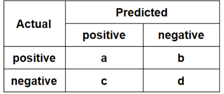
Confusion matrix is a table presenting the count of correctly predicted samples and incorrectly predicted samples, which can show the quality of a model on a dataset where the true labels are known. A confusion matrix of a binary classifier is shown in Figure 3.1. In a binary outcome case, the samples can be classified as positive or negative. True positives (denoted asa) is the number of correctly classified positive samples, and false negatives (denoted asb) is the number of wrongly classified positive samples. False positives (denoted asc) is the number of wrongly classified negative samples, and true negatives (denoted as d) is the number of correctly classified negative samples. [19,20]

Figure 3.1: Confusion matrix of a binary classification

The following metrics can be derived from the confusion matrix of a binary classifier, and they can assess a classifier in different views [19, 20]:

Accuracy = a+d a+b+c+d, (3.1) Sensitivity = a a+b, (3.2) Specificity = d c+d, (3.3) Precision = a a+c, (3.4)

F1 score = 2× P recision×Sensitivity P recision+Sensitivity =

2a

Equation 3.1 calculates the ratio of the correctly classified samples. It should be noticed that a high accuracy does not mean good performance of the model when the data set is imbalanced. Equation 3.2 is also known as Recall or True Positive Rate (TPR). TPR presents the percentage of positive samples predicted correctly out of all the positive samples. Equation 3.3, also called as True Negative Rate (TNR), indicates the ratio of correctly predicted negative samples among all the negative samples. Equation3.4 represents how often a sample is truly positive when it is predicted as positive. Sensitivity and Precision are inversely related to some degree, that is, increasing one will be highly possible to cause decreasing another one. Equation3.5is the harmonic mean of these two measures, looking for a balance between them.

Area Under the Receiver Operating Characteristic curve (AUROC) is a common measurement for a binary classification task. ROC curve is a plot of the TPR on the y-axis versus the FPR, defined as 1−Specificify = _{T N}F P_{+F P}, on the x-axis for various classification thresholds, which gives a visual summary of classification performance and describes relative trade-offs between true positives and false positives. The point (0,1) ((0%,100%)) indicates perfect classification where no incorrect predictions are made, and the diagonal liney=x represents the curve of a random guess. AUROC is the area under ROC, and it can show that when we randomly select a pair of samples from the data, how likely that the pair is correctly ranked (the positive sample is ranked higher than the negative one). A higher AUROC means a better model. [19, 23] The AUROC of an ideal classifier is 1, while that of a random guess is approximately 0.5 [24]. Figure 3.2shows three different ROC curves.

3.1.2 Machine Learning Workflow

A common machine learning workflow includes the following stages. • Problem Definition and Data Collection

First of all, we should define what problem needs to be solved and identify what data should be gathered. The quality and quantity of data determine possible model performances. In some cases there exists pre-collected data or even pre-processed data available, while in the other cases the data needs to be gathered from scratch or assembled from different sources. In this thesis, the raw data can be obtained from a website, so we do not need to collect it from the beginning. [19]

• Data Preparation

The data we collect in the first step is raw and unstructured, and it needs to be preprocessed before being input to models. It is possible that a particular order of data influences prediction results, so the order of data is randomised in such a case. The data cleaning includes error correction, removing duplicate data and irrelevant data, handling missing values, data transformation like normalisation and data type conversion, but not all of these are always needed. [26] Data exploration analysis (DEA) can be conducted at the same time. By DEA, a better understanding of data can be obtained, and the relationships between variables can be learned.

• Dimension Reduction and Feature Engineering

Too many features may cause overfitting and also increase computation cost. Moreover, some features may be unrelated to the target and disturb the prediction. Therefore dimension reduction is an effective step to improve models in many machine learning problems. Dimension reduction includes two parts: feature selection and feature extraction. The purpose of feature selection is to pick the most important features within the complete feature set. Filter methods, Wrapper methods and Embedded methods are three general classes of feature selection methods. Feature extraction involves transforming data into informative features. Principal component analysis (PCA) is one of the most common approaches of extracting features. The details about dimension reduction will be introduced in Section 3.3. Feature engineering, which is the process of constructing new features using domain knowledge, may help to improve the model performance in some cases. [19, 26, 27]

• Algorithms Choice (Model Training & Evaluation)

Many algorithms have been developed over the years. Some of them show good performance on image data; some algorithms are suitable for sequences like text, while others are good at handling numerical data. For different problems and different data set, the suitable algorithms are different. We can train a group of commonly used algorithms, performing cross-validation on the training data or testing on a holdout set, to determine which algorithms to use. One or

several algorithms which have relatively good performance can be selected for the further steps. [19, 26]

• Parameter Tuning and Model Selection

After deciding which algorithm(s) to use, we will further try to improve their prediction ability. Parameter tuning is an approach to realise that. An algorithm often has a set of model parameters can be adjusted, such as a regularisation term for a regularised logistic regression and a learning rate for a neural network, and adjustable parameters may be different for different models. We can try a collection of different parameter values and choose the one which gives out the best evaluation result. Grid search is a common parameter tuning technique and will be presented in Section 3.4. After tuning the parameters of each model, we can choose the best model or combine multiple models using ensemble methods. [19, 26]

• Deployment and Prediction

Finally, the optimised model is deployed to perform prediction on new unseen data. Generally, its performance in real-world applications will be evaluated by a test set. [19, 26]

It should be noticed that a few steps are interactive and several steps may be repeated many times. For example, selecting features using embedded methods is done during the process of training models; the data can be re-preprocessed and then the whole workflow can be repeated many times; the steps from Dimension Reduction and Feature Engineering to Parameter Tuning and Model Selection can be iterated until an acceptable model is worked out.

3.2

Algorithms

In this section, we will explain the classification algorithms chosen for our problem. They are Beta-binomial model (Section 3.2.1), Logistic regression (Section 3.2.2, Random forest (Section 3.2.3) and Boosting algorithms (Section 3.2.4). They have their own characteristics, and the mathematical theories behind them are different.

3.2.1 Beta-Binomial Model

The Beta-binomial model is the baseline model in our work. We will first ex-plain Bayesian inference, the fundamental theory behind the Beta-binomial model. Bayesian inference is a widely used statistical method which uses Bayes’ theorem to update a probability distribution on the parameters and estimate a probability point on unseen data conditioned on the observed data [28].

Bayes’ theorem can be expressed as:

P(B |A) = P(B)P(A|B)

where P(A) denotes the probability of the event A,P(B) denotes the probability of the event Y, P(A|B) is the conditional probability of A given thatB has occurred andP(B |A) is the conditional probability ofB given thatAhas occurred. By using Bayes’ theorem, we can infer the conditional probability based on the prior knowl-edge of conditions related to it. Bayesian inference is an application of Bayes’ theorem. When performing Bayesian inference, we first initialize a prior probability distribution of the unknown parameter θ, which is a reasonable guess and noted as p(θ) [33]. Then the posterior probability can be yielded based on the available data using Bayes’ Rule [28]:

Often, the probability of θ is called the prior, and the probability of data con-ditioned onθ is called the likelihood, written asp(data|θ). The joint probability is the product of the prior and the likelihood:

p(θ, data) = p(θ)p(data|θ). (3.7) Based on the Bayes’ Rule, the posterior probability can be obtained:

p(θ|data) = p(θ)p(data|θ)

p(data) , (3.8)

wherep(data) = Σθp(θ)p(data|θ). Since p(data) is independent from θ and can be

regarded as a constant when data is fixed, we can get the unnormalized posterior density:

p(θ |data)_∝p(θ)p(data|θ). (3.9)

Finally, the prediction can be done via some estimation methods such as Maximum Likelihood Estimation (MLE) or Maximum A Posteriori (MAP) estimation.

MLE selects the value of the parameter θ which gives the maximum likelihood function [34]:

ˆ

θM L = argmax θ∈Θ

p(data|θ). (3.10)

And in many cases, it is more convenient to maximize the natural logarithm of the likelihood (log-likelihood) [35]. MAP estimation finds the values of θ which maximize the posteriror probability [36]:

ˆ θM AP = argmax θ∈Θ p(θ |data) = argmax θ∈Θ p(θ)p(data|θ) p(data) = argmax θ∈Θ p(θ)p(data|θ). (3.11)

The difference between MLE and MAP is that MAP incorporates the prior knowledge while MLE does not. MAP can be regarded as regularisation of MLE, weighing

the likelihood based on the prior. When the prior is a constant, the prior could be ignored in the MAP target objective function, and thus the MAP is equal to MLE in this situation.

Let us talk about how Bayes’ theorem can be used in classification problems. Given an input datax, we aim to classify xas one of C classes. Supposing that ci is the

classiwherep(ci) is the prior class probability of classi,i∈ {1,2, ..., C}, andp(x|ci)

is the likelihood probability which is the probability ofx given that x belongs to class i, the posterior probabilityp(ci |x), the probability ofx belonging to class i

givenx, can be obtained using Bayes’ theorem [37, 38], p(ci |x) =

p(ci)p(x|ci)

p(x) , (3.12)

wherep(x) = ∑C

i=1

P(ci)P(x|ci). A decision rule is to classifyx as the class with the

highest posterior probability. The classifier using the rule is called Bayes classifier. [37] The error of the Bayes classifier is known as Bayes error, and it can be given as [37,38]: pBayes(error) = 1− C ∑ i=1 ∫ R_ci p(ci)p(x|ci)dx, (3.13)

where Rci is the region where class i has the highest posterior probability. The

equation shows that the Bayes classifier will minimize Bayes error. However, in most cases, it is impossible to obtain the Bayes error by the equation because of the difficulty in calculating the multi-dimensional integral, and thus the relevant studies focus on its approximation and its bounds estimation [37].

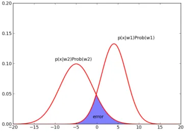
Figure 3.3 shows an example of a binary classification case where w1, w2 denote two

classes [39]. Choosing a value x0 as the decision boundary, the data on the left of

x0 is classified as w2 and the data on the right of x0 is classified as w1. The error

occurs in the intersection of the two curves, and it can be given as: pBayes(error) = ∫ Rw₂ p(x|w1)P rob(w1)dx+ ∫ Rw₁ p(x|w2)P rob(w2)dx. (3.14)

Theoretically the Bayes error can be zero if the classes are completely separable, i.e., for eachx if there exists a class k∈C such that p(ck |x)>0 then p(ci |x) = 0 for

every i∈C\ {k}. However, in practice, it is a very uncommon case. Generally, the Bayes error is non-zero and irreducible, even though we know the true probability distribution that generates data. The class distributions often overlap, and there may exist noises in the distribution, or some invisible variables that are not included the input may affect the output. [40] For example, we know the output of flipping a coin follows a binomial distribution, but we would still make errors when predicting the output of a series of coin flips since the process is inherently stochastic.

The Bayes error provides the minimum prediction error an optimal classifier could achieve for a given machine learning problem [37], which means that the optimal prediction error of any classifiers could be close to but never smaller than the Bayes error. The optimal classifier is typically unknown, and generally, we choose a collec-tion of classifiers denoted as_L and want to find an optimal classifier l∗ from _L so thatpBayes(error)≤pl∗(error). In this thesis, the collection of classifiers we choose include Beta binomial model, Logistic regression, Random forest and LightGBM, and they will be introduced in this chapter later. Given a data set with a finite size, the prediction error rate of each classifierlin_Lis evaluated by the given data and denoted as pl(error |data), and then the estimated optimal classifier will be the one with

the lowest value ofpl(error |data). Therefore, we havepl∗(error)≤p_l(error|data). The values of pl(error |data) are random variables since they depend on the given

data coming from an underlying distribution and generated through an inherently stochastic process. Besides, we can not get the exact values of pl(error | data)

but compute their estimates ˆpl(error |data) by certain error estimation methods,

such as cross-validation and bootstraps (which will be introduced in Section 3.2.3). These computed estimates are also random variables existing variance because of the dependence on the given data and the variation during the error estimation process, e.g., the randomness of data splitting on the cross-validation procedure.

Now let we start to discuss Beta binomial distribution, which is a compound distri-bution of the Beta distridistri-bution and the binomial distridistri-bution. In many cases, an experiment produces binary outcomes, e.g., coins will land either heads up or tails up after being flipped. Generally two different outcomes can be defined as ’success’ with probability p and ’failure’ with probability q = 1−p. Each trial of such an experiment is called a Bernoulli trial. [41] A binomial model is a statistical model which has the following properties: 1. it contains a set of repeated Bernoulli trials. 2. The trials are exchangeable, which means that their joint probability does not change

if they are permuted. 3. The trials are independently and identically distributed; that is, they are not affected by each other and follow the same distribution. [28,42] The binomial distribution, denoted as K ∼ Bin(n, π) models the the number of successes K in n trails with a probability of success π in a trial. The probability mass function gives the probability of k successes:

P r(K =k |n, π) = ( n k ) πk(1−π)n−k, k = 0,1, ..., n, (3.15)

where n∈_N, π∈[0,1]. For a binomial random variable K with parameters n andπ, the expectation is E(K) = nπ and the variance is Var(K) =nπ(1−π).

A beta function is defined as: B(α, β) =

∫ 1 0

tα−1(1−t)β−1dt= Γ(α)Γ(β)

Γ(α+β), α, β >0, (3.16) where Γ(α) is the gamma function, Γ(α) =∫∞

0 t

α−1_e−t_{dt forα >0.}

The beta distribution denoted as Beta(α, β) is a continuous probability distribution with two positive parameters α and β. Its density function is:

f(x;α, β) = ⎧ ⎪ ⎨ ⎪ ⎩ 1 B(α, β)x α−1_(1−x)β−1_{, x∈[0,1];} 0, otherwise. (3.17) The mean of a random variable X that follows the distribution Beta(α, β) is E(X) = α

α+β, and its variance is Var(X) =

αβ

(α+β)2_{(α+β+ 1)} [33].

The beta binomial distribution is a hierarchical model which has multiple parameters connected in different levels. [28] More specifically, it is the binomial distribution where the probability of success in a trail π is beta-distributed with α, β:

The prior of p follows the Beta distribution: π∼Beta(α, β),

p(π)_∝πα−1(1−π)β−1. (3.18) The likelihood is defined as:

K ∼Bin(n, π), p(k|n, π)_∝πk(1−π)n−k, p(k|n, π) = ∫ p(k, π |n, α, β) = ∫ p(k |π, n)p(π |α, β)dπ = ( n k ) 1 B(α, β) ∫ 1 0 πk+α−1(1−π)n−k+β−1dπ = ( n k ) B(k+α, n−k+β) B(α, β) . (3.19)

The posterior for π is

p(π |n, k)_∝πα−1(1−π)β−1πk(1−π)n−k =πα+k−1(1−π)β+n−k−1 =Beta(α+k, β+n−k).

(3.20)

Equations3.18 and 3.20 show that if the prior is a beta distribution and the likeli-hood is a binomial distribution, then the generated posterior will be a distribution whose parametric form is the same as that of the prior. The beta distribution is a conjugate prior for the binomial distribution [28]. A conjugate prior is convenient for computation, since the posterior is in a known form and we do not need to compute the integrals.

3.2.2 Logistic Regression

Logistic regression is a well-known algorithm for the purpose of classification. It estimates the relationship between the features and the target via a logistic function. It is very easy to understand and implement, and shows great performance on linearly separable classes, so it is widely used in diverse fields including biostatistical problems. [26] Since our work is a binary classification task, here we just discuss the binary logistic regression, but it can be extended to multiclass problems.

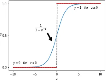
Considering a binary classification task, the input containingdfeatures is denoted as x= (x1, x2, ...xd)T and the label is y ∈ {0,1}. Let p∈(0,1) denote the probability

of the positive event, thus 1−p∈(0,1) is the probability of the negative event. The log odds, denoted as log(p/(1−p)), is the logarithm of the odds of probabilities. The log odds is modeled by linearly combining features:

logit(p) = log p

1−p =w0+w1x1+w2x2+...+wdxd=w0+w T

x, (3.21) wherew = (w1, w2, ..., wd)T. When logit(p)>0 which means p > 1−p, the sample

is classified as 1, while it is predicted as 0 iflogit(p)<0. So the outcomey of logistic regression is determined as follows:

y= ⎧ ⎪ ⎨ ⎪ ⎩ 1, w0+wTx>0; 0 or 1, w0+wTx= 0; 0, w0+wTx<0. (3.22)

When logit(p) = 0, the sample can be set to be classified as 0 or 1. [20] Based on Equation 3.21, we can estimate the conditional probabilities

P(y = 1|x) = 1 1 +e−(w0+wTx), P(y = 0|x) = 1−P(y= 1|x) = e −(w0+wTx) 1 +e−(w0+wTx). (3.23)

Figure 3.4 shows a typical logistic regression curve, wherez =w0+wTx, the blue

curve shows the trend ofP(y = 1|x) and the red lines denote the decision function of classification. [20]

Figure 3.4: a logistic regression curve

MLE is used to estimate the coefficientw0 and w. We denote the estimated P(y=

1|x) as hw_{(x), and then we can get the probability of y conditioned on x,}

P(y|x) = [hw(x)]y[1−hw(x)]1−y. (3.24) For a dataset X containing N samples, w can be obtained by maximizing the log-likelihoodl(w|y,X) = log ∏N

i=1

P(y(i) _|x(i)_{) where X = (x}(1)_,x(2)_...,x(N)₎T _and

y= (y(1)_{, y}(2)_{..., y}(N)₎T_{. It is equivalent to minimizing its negative form, which is the}

loss function of logistic regression called log loss and denoted asJ(w). [20]J(w) is written as J(w) = −log N ∏ i=1 P(y(i)|x(i)) = N ∑ i=1

−y(i)loghw(x(i))−(1−y(i)) log(1−hw(x(i))).

(3.25) So w∗ = argmin w N ∑ i=1

{−y(i)_loghw_(x(i)_)−(1−y(i)_{) log(1−h}w_(x(i)_))}

= argmin w N ∑ i=1 {−y(i)_(w 0+wTx(i)) + log(1 +ew0+w T_x(i) )}. (3.26)

Some optimization techniques can be adopted to solve this minimization problem, such as gradient descent method or Newton-Raphson method [20, 29]. When using

the gradient descent algorithm, first we initialize wj as 0 or a random value for

j = 1,2, ..., d. The derivative of J(w) with respect to wj is

∂J(w) ∂wj = N ∑ i=1 (hw(x(i))−y(i))x(_ji), (3.27)

which is easy to compute. Then wj is updated by

wj =wj−η

∂J(w) ∂wj

, (3.28)

where η ∈ (0,∞) is a learning rate that decides the update size in each step. An overhigh value of η possibly leads to missing minimum points or failing to converge, and an excessively lowη may make the computation expensive. Therefore η needs to be carefully chosen. The update is iterated until satisfying a stopping condition, such as reaching the maximum number of iterations or satisfying a tolerance value. As we mentioned in Section 3.1.1, when d >> N, the model is prone to over-fitting. For a linear model, regularization is a useful technique to solve this problem. A norm penalty term that shrinks coefficients is added to the loss function:

J(w) =−log

N

∏

i=1

P(yi |xi) +λ∥w∥rr for r= 1 or 2, (3.29)

where ∥w∥r is the r-norm of w, and λ∈[0,∞) is a manually predefined parameter

that decides how much the coefficients are penalized. Note that w0 does not need to

be penalized since it does not influence weights of features and thus does not induce overfitting. λ is manually set, and the largerλ is, the more heavily the coefficients are penalized, leading to more coefficients close to zero. When λ is 0, the model is the logistic regression without regularization. Cross-validation is often used to find an optimal value of λ. [20, 21, 29]

Whenr = 2, the penalty term isL2 norm, and it is referred to as Ridge regression

or L2 regularisation. Ridge regression prevents the weights from rising too high and drives them to be small. L2 is differentiable, and therefore it can be solved by

gradient descent algorithm. While r = 1, the penalty term is L1 norm and it is

called Lasso regression or L1 regularization. Lasso regularisation can drive some coefficients of features to zero, and these features will not contribute toy. Therefore it will make the solution more sparse compared with Ridge regression and can be used as a feature selection technique. L1 is non-differentiable, and thus Lasso has

no analytical solution, but it can be solved by certain algorithms such as Proximal Gradient Descent. [20, 21,29]

We can also apply the logistic regression using a Bayesian approach, and such an algorithm is called Bayesian logistic regression. A prior forw is initialised, and the Gaussian distribution is a common choice. Then we can perform Bayesian infer-ence described in Section3.2.1. There is no closed form for the predictive posterior,

but some methods, such as Laplace Approximation, can be used to approximate it. [30] Moreover, now there exist automatic software or packages such as Stan or PyMC3 can compute these posteriors using simulation.

3.2.3 Random Forest

Random forest constructs a group of decision trees and ensembles them using Bagging method. Therefore we first have a look at the decision tree and Bagging algorithm and then discuss the random forest. Note that since our work is a classification problem, here only classification models are discussed.

The decision tree is a tree-like model, where the root contains the whole feature set, each internal node is a feature, each branch denotes a rule based on the feature value, and each leaf is a class label. It classifies an instance from the root (top) down to a leaf (bottom) by testing a sequence of features. A path from the root down to a leaf can be explained as a collection of if-then rules pointing to a class label, and thus the decision tree is easy to understand and interpretable. [20] An example of a decision tree is illustrated in Figure 3.5.

Figure 3.5: A simple example of decision tree [19]

There are different types of decision trees, but the general approach of decision tree learning can be summarised as follows: 1. At a node, the best feature is selected as the decision feature from the feature set. The best feature is the one that can best separate the data, which is measured by a splitting criterion. 2. The data is partitioned into smaller subsets and distributed to the new child nodes, based on certain cutoff values of the decision feature. Then the decision feature is re-moved from the feature set. 3.Repeating the steps 1-2 for each node until satisfying a stop criterion such as the depth of the node is equal to a preset threshold. [19,20,21] Information gain is a commonly used splitting criterion. Assuming that for a dataset X, the samples with the label c is X(c) and the proportion of X(c) is pc = X_X(c),

H(X) = ∑

c∈C

−pclog2pc is the information entropy of the dataset X. It measures

the purity of data, and a lower information entropy means a higher purity. If all the samples belong to the same class, the information entropy of the data is 0. The information gain of feature A on the dataset X is defined as

IG(X, A) = H(X)− ∑

a∈A

|Xa|

|X|H(Xa), (3.30)

whereXa is the subset containing the samples with the feature valuea. A feature has

larger information gain means that it can improve classification more if it is chosen as the decision feature. The ID3 algorithm uses information gain as its splitting strategy, and the feature that has the highest information gain is selected as the splitting point. [19, 20]

Another popular splitting criterion is the GINI index. The GINI impurity is a metric evaluating the impurity of the data. Using the same notation as the above, Gini(X) = ∑ c∈C ∑ c′_∈C\{c} pcpc′ = 1− ∑ c∈C p2

c. The lower GINI value is, the purer the data

is. The Gini index of feature A on the dataX is GI(X, A) = ∑

a∈A

|Xa|

|X|Gini(Xa). (3.31)

The Gini index indicates how mixed the classes are after the data is split by the feature. If the data is separated perfectly, the Gini index will be 0. Classification And Regression Tree (CART) divides a node based on the feature with the lowest GINI index. [19,20]

We should notice that the decision tree is prone to suffer from the overfitting problem, especially if there exists noisy data or irrelevant features. To prevent overfitting, we can early stop growing a tree when meeting some certain stopping criteria, e.g., the depth of the tree is limited by a predefined maximum number, or there are some pruning techniques can be used. [21] Another problem is that the decision tree is a high-variance model, and small fluctuations in the data might cause a totally different tree is generated. Besides, since the decision tree learning is greedy, it can not be guaranteed that the generated model is globally optimal.

Bagging, also called Bootstrap aggregating, is a machine learning ensemble method which trains a set of homogeneous classifiers by bootstrap samples and then ensembles them to generate outputs. Bagging first produces a set of bootstrap samples, each of which is produced by randomly sampling with replacement from the training set, and the number of samples in each bootstrap sample is the same as that of the training set. Then a base classifier is trained on each bootstrap sample separately. Finally, combining the outcomes of this collection of classifiers using a certain strategy to generate the prediction for a sample. [19]

For classification problems, a voting strategy is used to make final predictions. Majority voting is a common and simple strategy which has three versions: 1. the output class is the one that is agreed by all classifiers (unanimous voting) [19].2.the final prediction is the class that receives more than half of the votes (simple majority) [19, 31]. 3.the class that get the highest total votes is chosen (plurality voting) [31]. In addition to the majority voting, the weighted voting is another often used strategy. The contribution of each classifier to predictions is weighted, and the weights can be decided in a self-defined way [20, 31].

We are often interested in estimating class-probabilities instead of class-labels, or we prefer to classifying samples to the class whose class probability are highest. The class-probabilities are combined by averaging them over all the classifiers, which is called soft voting. For a tree, the class probability is the percentage of samples of the class in the leaf. Soft voting can improve the estimates of class-probabilities and produce bagged classifiers with lower variance. [29]

Figure 3.6: An illustration of Bagging framework[45]

Figure3.6 shows how Bagging works. Bagging is an efficient algorithm since it trains multiple classifiers in parallel and thus has the same level of time complexity as training a single model. For a bootstrap sample with the same sample size as the complete dataset, there are around 63.2% of unique samples while the other 36.8% are the replicates. Those 36.8% samples in the original data that do not appear in the bootstrap sample are out-of-bag (OOB) examples. OOB examples can be used to evaluate how good the generalisation ability of the model is, which is called OOB estimate. [20, 19] Since bootstrap samples are slightly different from each other, a set of different classifiers can be produced. Combining multiple classifiers can help to decrease variance and prevent overfitting, and therefore Bagging is suitable for high-variance models such as decision trees. [19, 29]

Random forest is a variant of Bagging. It uses the unpruned decision tree as the base classifier. The difference happens in the process of decision tree training: at the node to split, not the whole feature set but a subgroup of the features is randomly chosen as the candidates, and the best one is chosen as the decision feature among them. Since there are fewer features to evaluate, the training process is speeded up. Moreover, it adds randomness in the training of each tree, which increases the variance between different trees and then possibly improves the generalisation ability of the classifier. [19] For a classification problem, at a node withd features, typically log₂d features are selected as splitting candidates [29].

In a random forest, the feature importance can be evaluated by ’mean decrease in impurity’ or ’mean decrease in accuracy’ mechanism. The ’mean decrease in impurity’ sums the impurity decrease every time the feature is selected as the split point across every tree, and then averages it across all the trees. The more mean decrease in impurity is, the more significant the feature is. Another method ’mean decrease in accuracy’ measures the effect of the feature on the model accuracy. For each tree, it randomly permutes the feature values in the OOB samples and measures the decrease in accuracy after permutation. The mean decrease in a forest is obtained by averaging the decreases over all the trees. A lower the mean decrease in accuracy means that the feature has less effect on the model accuracy, and therefore the less important the feature is. [29,32]

3.2.4 Boosting

Boosting is a collection of ensemble algorithms which combines a collection of weak homogeneous classifiers into one strong classifier. Different from Bagging, a boosting algorithm trains a group of base classifiers sequentially. Each base classifier is trained using a data set which is weighed by the prediction made by the previous classifiers. More specifically, in each round, the misclassified samples are given heavier weights in the newly weighed data set used for the next training. The final prediction is given by combing the classifiers through a weighted majority voting strategy, where models that have lower error rate are given more weights. The Boosting framework is showed in Figure 3.7. [29, 30]

Figure 3.7: An illustration of Boosting framework [30]

Adaptive Boosting (AdaBoost) is a commonly used boosting algorithm. Given a datasetD ={(x1, y1),(x2, y2), ...,(xn, yn)} and yi ∈ {−1,1}, we denote the initial

weight of the data point xi as w1i and set it as 1/n, and fix the number of base

classifiersM. Form = 1,2, ..., M, the classifier hm(x) is trained sequentially, aiming

to minimizing the weighted loss function Jm =

n

∑

i=1

wm_i I(hm(xi)̸=yi). (3.32)

Then the weighted error rate of hm(x) can be calculated by

ϵm = n ∑ i=1 wm i I(hm(xi)̸=yi) n ∑ i=1 wm i . (3.33)

Computing the weight of the classifier using this error rate by the formulahm(x)

αm = 1 2ln 1−ϵm ϵm . (3.34)

The weights of the data points are updated by w_im+1 = w

m

i exp (−αmyihm(x))

Zm

, (3.35)

where Zm is a normalization factor that makes sure all the weights sum up to 1.

After M classifiers being trained, the prediction is made by H(x) =sign(

M

∑

m=1

Equation 3.34 shows that a base classifier that has a lower weighted error rate is assigned a greater weight when performing predictions. From Equation 3.35 we can see that those samples wrongly predicted are given more weights more while the other samples correctly predicted are given less weights, and then subsequent classifiers will more focus on samples that have been misclassified before. [19,29,30] Another boosting method is Gradient boosting, which is popular in recent years and shows a strong power. It is widely used in the learning to rank field [43], e.g., Frery et al.(2017) adopted gradient boosting algorithms to solve a anomaly detection problem in a learning to rank approach [44]. Given a dataset D = {(x1, y1),(x2, y2), ...,(xn, yn)}, a loss function L(y, H(x)) that is differentiable, and

the number of iterationsM, we aim at finding a function H∗(x) which makes the loss function minimized:

H∗(x) = argmin

H

Ex,yL(y, H(x)). (3.37)

To optimize the cost function, repeatedly choosing a weak hypothesis that points to its negative gradient direction. Firstly an initial model H0(x) is generated. For

m= 1,2, ..., M andi= 1,2, ..., n, the residual of each sample is computed using the formula rim=− [∂L(y_i, H(x_i)) ∂H(xi) ] H(x)=Hm−1(x) . (3.38)

Then a base classifier hm(x) is trained using the dataset{(x, ri)}ni=1. The multiplier

γm can be obtained by γm = argmin γ n ∑ i=1 L(yi, Hm−1(xi) +γhm(x)). (3.39)

The model is updated by

Hm(x) = Hm−1(x) +γmhm(x). (3.40)

After M iterations, the HM(x) is the finally classifier. [29,46]

In this thesis, we applied a boosting algorithm called LightGBM. LightGBM is a further improved algorithm. It optimises computation speed and memory usage by histogram-based algorithms, and the Gradient-based One-Side Sampling and Exclusive Feature Bundling techniques can help handle big data with faster speed and less memory consumption. The trees of LightGBM are grown leaf-wise while the other algorithms grow trees level-wise, which makes LightGBM more accurate but also prone to overfitting when the data is small. LightGBM also supports parallel learning. [48]

3.3

Feature Selection

Feature selection aims to choose features that are most relevant for predicting the target from the complete feature set. By removing irrelevant or redundant features,

feature selection helps simplify constructed models, avoid the curse of dimensionality, improve the performance of classifiers and reduce computation space and time [49]. It also assists in understanding data, e.g. learning about the critical factors that affect the relationship between the object and the target. Feature selection is an significant step in implementing machine learning, especially in the case that data is high-dimensional. In our case, the features are a vast number of TCRβ sequences and plenty of them are not related to the target phenotype, so it is necessary to select an appropriate feature subset before training machine learning models. Feature selection approaches mainly consists of filter methods, wrapper methods and embedded methods.

3.3.1 Filter Methods

Filter methods score and rank each feature in the original feature set by a selected statistical test which assesses the feature relevance with the label and then remove those features whose scores are below a manually set threshold. They are indepen-dent of machine learning algorithms, and since they do not take the relationships between features into account and may therefore select redundant features, they are often the first action in the stage of feature selection. [49] There are vari-ous statistical criteria could be used to assess features. In this thesis we used the Fisher exact test to filter features firstly before trying other feature selection methods. Fisher exact test is a statistical measure for assessing the association between two categorical variables by analyzing their contingency table. It is suitable for analyzing small data set [50]. The contingency table is a table displaying the frequency dis-tribution across two nominal variables, and the 2×2 contingency table is the most applied case for inspecting the relationship between a feature and the target variable:

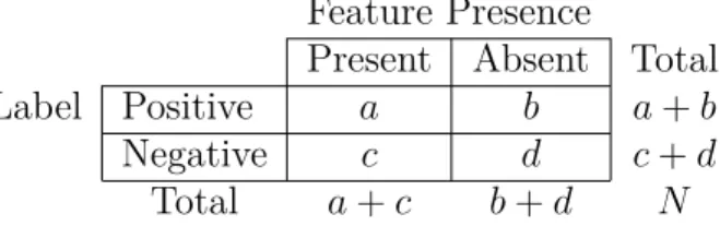
Feature Presence

Present Absent Total Label Positive a b a+b Negative c d c+d

Total a+c b+d N Table 3.1: An example of a 2×2 contingency table

The null hypothesisH0 of Fisher exact test is that the two variables are independent.

The p-value is the total probability over all the tables which have the probabilities equal to or smaller than that of the observed condition under the null hypothesis. It is computed using the formula [51]

p= (a+b)!(c+d)!(a+c)!(b+d)!

a!b!c!d!N! . (3.41)

A lower p-value indicates a higher significance that the null hypothesis could not explain the observation. If the p-value is lower than a chosen threshold α known