Network and Cascade Representation Learning: Algorithms based on Information Diffusion Events

(1)

DEPARTMENT OF INFORMATION ENGINEERING AND COMPUTER SCIENCE

ICT International Doctoral School

Network and Cascade

Representation Learning

Algorithms based on Information Diffusion Events

Zekarias Tilahun Kefato

Advisor

Prof. Alberto Montresor

Universit`a degli Studi di Trento

(2)

(3)

Dedicated to

my father Tilahun Kefato

and

(4)

(5)

Abstract

Network representation learning (NRL) and cascade representation learn-ing (CRL) are fundamental backbones of different kinds of network analysis problems. They are usually carried out in settings where the structure of the network under consideration is known. Motivated by real-world prob-lems, this study presents several algorithms for scenarios where the network structure is partially or completely unknown.

The objective of network representation learning is to identify a mapping function that projects sparse and high-dimensional network graphs into a dense latent representation, which preserves the original information about nodes and their neighborhoods. The notion of neighborhood, however, be-comes illusive when the network structure is partially or completely hidden.

Inspired by previous results, in our thesis work we have developed novel algorithms that are resilient to such lack of knowledge. These results estab-lish a correlation between the properties of the network and different kind of node activities performed over it, information which is generally more available and can be easily observed. In particular, we focus on diffusion events – also called cascades – such as shares, retweets and hashtags.

In the first of our contributions, we have developed a novel NRL algorithm called _Mineral, a simple technique that combines the observed cascades with the partially accessible network structure by sampling artificial cas-cades. Node representation is then learned from the observed and sampled cascades by using the _SkipGram model that is widely used for word

(6)

rep-6

resentation learning in natural language documents.

In our second contribution, called _NetTensor, we assume that the net-work structure is completely hidden and we propose novel techniques that are capable to estimate both the hidden neighborhood (proximity) and the similarity of nodes. Such estimated values are then used to learn a unified embedding of nodes using a scalable truncated singular value decomposition and deep autoencoders.

In addition to the NRL algorithms, we have also proposed a novel CRL algorithm called _cas2vec for virality (popularity) prediction. Again, we pursue a network-agnostic approach following the above assumption that the network structure is completely unknown. Unlike prior studies that rely on manual feature extraction, _cas2vec automatically learns cascade representations based on convolutional neural networks, that are effective in predicting virality of cascades.

We have carried out extensive experiments using several real-world datasets for all of our methods and compared them against strong baselines from the state-of-the-art, achieving significantly better results than many of them.

Keywords

[Network representation learning, information diffusion, deep learning, ma-trix factorization, social network analysis, cascade prediction]

(7)

List of Tables

2.1 Notations and Conventions . . . 16

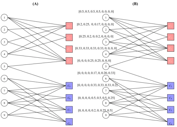
4.1 Cascades extracted from observed hashtag use of nodes of the social network in Fig. 4.1(A). A cascade is constructed by sorting nodes according to the time stamp that they have

used a particular hashtag. . . 38 4.2 Summary of the datasets . . . 43 4.3 Results for the link prediction task on the Twitter dataset 45 4.4 Results for the link prediction task on the Memetracker dataset 45 4.5 Results for the link prediction task on the Flickr dataset . 45 4.6 Node classification accuracy on different levels of labeled

training set ratio for the Twitter dataset . . . 46 4.7 Node classification accuracy on different levels of labeled

training set ratio for the Memetracker dataset . . . 46

5.1 Dataset summary. . . 73 5.2 Edge feature construction techniques. Φ[uv] is an edge

fea-ture vector for a pair of nodes u, v ∈ V and Φ[uv, i] is the

ith component. . . 73 5.3 AUC score for link prediction with rate = 30%. Bold

indi-cates the best performing algorithm for a dataset and un-derline indicates the best performing feature construction

technique for each dataset and each algorithm. . . 76

(12)

LIST OF TABLES vi 5.4 AUC score for link prediction, with rate = 50% and

Aver-age edge feature learning method. Bold indicates the best

performing algorithm for a dataset. . . 77 5.5 P@K results for the network reconstruction task, λ = 1. . . 78 5.6 P@K results for the network reconstruction task, K = 500K. 78 5.7 Micro-F1 results for node classification alongside the

stan-dard deviations with 95% confidence interval. . . 81 5.8 Macro-F1 results for node classification alongside the

(13)

List of Figures

1.1 An example social network . . . 4 1.2 A subgraph of the social network in Fig. 1.1. . . 4

3.1 Architecture of the neural-non-negative matrix factorization model. Dotted lines indicate optional components. If the dotted box is left out, the NNMF is equivalent to NMF and

instead of concatenation we compute dot product. . . 21 3.2 Architecture of the _SkipGram model . . . 23 3.3 A standard architecture of an autoencoder. Each units of

the feed-forward network constitutes a non-linear activation (f) of the linear transformation P

of its input. . . 26 3.4 CNN model for sentence classification . . . 28

4.1 An example of a complete social network (A) and possible subgraphs (B) and (C) that could be crawled as a result of privacy settings of nodes. (B) If only node 2 have set its connection setting to private; and (C) if 3 have also decided

to go private on its connections alongside 2. . . 36 4.2 Multi-label classification (using one-vs-rest logistic

regres-sion classifier) on the Blogcatalog dataset . . . 47 4.3 Multi-label classification (using one-vs-rest logistic

regres-sion classifier) on the Flickr dataset . . . 47

(14)

LIST OF FIGURES viii 4.4 Visualization of top-5 communities with at most 2000 users

in the Twitter Dataset using (A)_Mineral(B) _DeepWalk

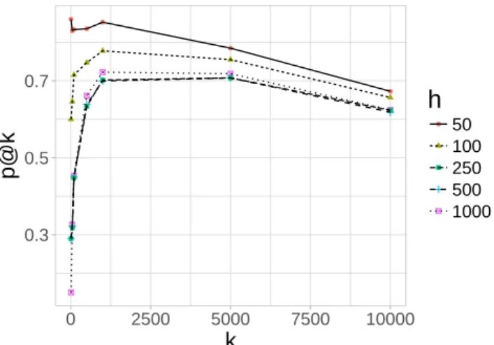
and (C) Line . . . 49 4.5 Sensitivity of the parameter h using the link prediction task

on Blogcatalog . . . 49

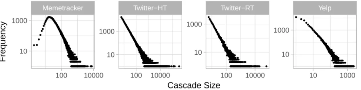
5.1 Cascade size distribution for the datasets used in our

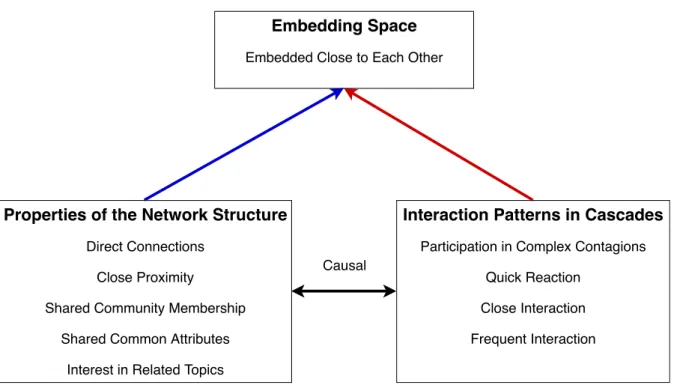
exper-iments . . . 54 5.2 Relations between properties of a network structure,

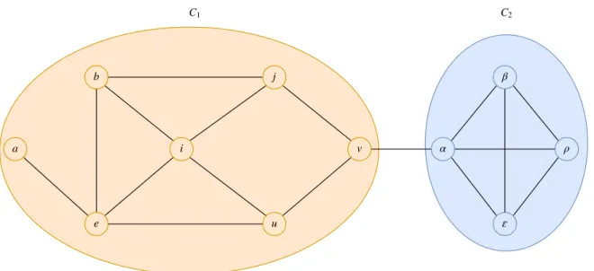
inter-action patterns in diffusion events and an embedding space 55 5.3 An example graph with two communities, C1 and C2. . . . 56 5.4 User-cascade bipartite graph illustration. Two groups of

users discussing about the AC Milan football club and Ethiopian politics . . . 62 5.5 Relations between local context and topic feature

extrac-tions. The former method uses a bipartite graph in (A). Similarly the latter one can be modeled as a weighted bi-partite graph by taking the rows of the transformed event

matrix E0 to put weights on the edges . . . 65 5.6 Topic (A), where order matters, vs. local context (B)

fea-tures, where order does not matter. (A) is plotted form LF

and (B) from TF. . . 67 5.7 _NetTensor Framework . . . 70 5.8 Performance of Node Models in Link Prediction. . . 82 5.9 Performance of Node Models in Network Reconstruction,

λ = 2 and K = 500K. . . 82 5.10 Performance of the two kinds of features in the three types

(15)

LIST OF FIGURES ix 5.11 Effect of proximity window, local context window, and

em-bedding sizes, AUC and P@K are the scores for link predic-tion (Link Pred.) and network reconstrucpredic-tion (Net. Rec.),

respectively. . . 85 5.12 Effect of the final embedding size d on node classification . 85

6.1 Examples of two recent hashtag campaigns. (A) The tweet-ing frequency of each hashtag; #metoo achieved more spread compared to #gamergate. (B) The network properties of the participating nodes in each hashtag in terms of average number of followers; the nodes engaged in the first 12 hours

almost achieve similar reachability in both hashtags. . . 91 6.2 Two slices of size 2 hours, applied to the user coverage

dis-tribution of a viral hashtag (#thingsigetalot) and a non-viral one (#bored), which have reached 13711 and 43 users

in an observation window size of 4 hours. . . 98 6.3 Constant sequence as a step function . . . 100 6.4 The distribution of the user coverage for the viral and

non-viral classes. The user coverage distribution is computed at observation time to as |C(to)| and virality is computed at

prediction time to + ∆. A cascade is viral if |C(to + ∆)| ≥

1,000 and not-viral if |C(to + ∆)| < 1000 . . . 101

6.5 The CNN model adopted for cascade prediction . . . 102 6.6 Virality prediction results for both of our datasets. For

Twitter, filter sizes = 3, 5, 7 and for each filter we have 16 of them. For Weibo, filter sizes = 2, 4, 5, 7 and for each filter we have 64 of them. For both datasets, the size of the embedding matrix is 128, the number of units in the fully

(16)

LIST OF FIGURES x 6.7 Evaluation results of early prediction experiments for the

Twitter and Weibo datasets. The prediction time is fixed to 16 hours for Twitter and 34 hours for Weibo, and the same

hyper-parameter values as Fig. 6.6 is used . . . 108 6.8 Break-out coverage for k = 100 and k = 200 for the Twitter

dataset. . . 109 6.9 Break-out coverage for k = 10 and k = 20 for the Weibo

dataset. . . 110 6.10 Effect of the number of slices on virality prediction at to = 1

hour and ∆ = 12 hours. . . 111 6.11 Effect of sequence length on running time. . . 112 6.12 Effect of sequence length on virality prediction. . . 112

7.1 _Harp’s Graph coarsening techniques (A) - edge coarsening

and (B) - star coarsening . . . 118 7.2 _sdne model . . . 119

(17)

Chapter 1 Introduction

Graphs are widely used to model sets of entities that interact over a given medium, such as users in social networks, blogs over the Internet, proteins in biological networks, locations in road networks, and so on. Efficiently representing the entities (nodes) and their interactions (edges) is a critical step towards performing meaningful analysis over such complex networks. Graphs are usually represented “as is”, using basic data structures such as adjacency or incidence matrices. For example, an adjacency matrix

M∈ [0,1]n×n, where nis the number of nodes, is such that M[i, j] captures the existence (1) or the absence (0) of an edge between node i and j. Despite its simplicity, performing some kinds of tasks (e.g., link prediction or node classification) based on such complete representation usually leads to poor performance; the resulting computation can be very expensive depending on n, commonly known as the curse-of-dimensionality.

For this reason, alternative techniques have been designed to encode graphs in more compact and efficient ways. Consider an encoding oracle

O : [0,1]n×n → _Rn×d_{, which transforms a complete representation} _M _into

an encoded representation Z = O(M), where d n.

Zis a compact and dense representation obtained by applying the oracle

O such that the “most important” properties ofM are preserved inZ. The

(18)

2 problem of network representation learning (NRL) or graph embedding amounts to identifying the oracle O.

In the last few decades, several strategies have been proposed towards this goal. The classical approaches are based on explicit matrix factor-ization, such as latent semantic indexing (LSI) [14], non-negative matrix factorization (NMF) [60, 49], or singular value decomposition (SVD).

More recent approaches utilize artificial neural networks and can be subdivided in two main groups. On one hand, some studies seek to preserve the local and/or global properties of nodes [64, 70, 28, 77, 19, 32, 1, 59, 45, 29, 44]. Potential properties of interest are first-order, second-order, and in general higher-order proximities of nodes, or cohesive structures such as community subgraphs, etc. These approaches are usually suitable to preserve similarities (homophily) between nodes.

On the other hand, some complementary studies have endeavored to pre-serve the role of nodes, such as being hubs, bridges or peripheral nodes [32, 19, 1, 45, 30].

In addition to the aforementioned works, recent studies have been pro-posed to take advantage of additional aspects of graphs, as well. In the early stage of the neural network representation learning (NNRL), sev-eral papers have exploited the network structure only [64, 28, 70, 77]. Follow-up studies have proposed to incorporate node attributes and have empirically proven that such approach leads to a better quality represen-tation [85, 34, 55, 66].

Furthermore, alternative studies [9, 38, 39, 40] have also been proposed to exploit explicit interaction between nodes of a network. In particular, these studies have focused on interactions that led to information diffusion events. The main advantage of these studies is that their methods can be used for predicting the future state of the diffusion events themselves (cascade prediction).

(19)

1. INTRODUCTION 3 The focus of this thesis is on the use of information diffusion events in order to achieve network and cascade representation learning (NRL and CRL, respectively). Towards this end we follow two main directions: on one hand, we consider scenarios where the network structure is partially or completely known; on the other hand, we consider scenarios where the network structure is hidden. In particular, we give more emphasis to the latter case.

While the entire study could be motivated by the list of applications presented in Section 1.3, we first highlight why we need techniques based on diffusion events when the network structure is partially or fully hidden.

1.1 Motivation

Existing studies dedicated to both NRL and CRL are heavily reliant on the network structure. This is, however, a problem as there are several cases where one might lack the complete or partial structure of the network.

For example, consider online social networks (OSN) such as Twitter and Facebook. The follower/friend links on these networks are usually very difficult to obtain by interested third parties (researchers or businesses) working outside the OSN host companies, due to privacy policies and com-petitive market advantages [2]. Even when the data is publicly available, it may take several months to extract just a portion of the network. Another scenario could be an epidemic, where we know who has been infected and

when, but not how they got infected.

Motivating example: Let us consider an excerpt of a hypothetical

friend-ship subgraph of a Facebook like social network depicted in Fig. 1.1. Users of such social networks normally have the possibility to make their friend-ship links private, and hence let us suppose 2, 3, and 9 have done so.

(20)

1.1. MOTIVATION 4 2 3 4 6 Text 7 8 9 10 5 1

Figure 1.1: An example social network

2 3 4 6 7 8 9 10 5 1

Figure 1.2: A subgraph of the social network in Fig. 1.1.

Now, consider a particular startup company xyz plc that wants to use the friendship network of the above social network for some of its services. A developer from xyz plc crawls the friendship network; the best she can manage to obtain, however, is the graph that is shown on Fig. 1.2, due to the privacy policy. Any representation R learned over such graph is apparently far from what one desires to achieve. We need to carefully ex-amine other sources of information that might enable us to achieve a better

(21)

1. INTRODUCTION 5 representation than R.

Fortunately, previous studies have shown a strong correlation between the dynamics of information diffusion events and the network structure [82, 83]. That is, in most diffusion events, similar users have the tendency to participate together. For example, if two users are connected, then they have a better likelihood of being involved in similar diffusion events with respect to a random user that is not connected to them. Therefore, one can use diffusion events as a proxy to the network structure by carefully probing the aforementioned kinds of correlations.

As a result, it is imperative to design representation learning algorithms – for both network and cascade prediction scenarios – that are not depen-dent on the knowledge of the complete network structure, but are still ca-pable of producing “very good” results using information diffusion events.

1.2 Research challenges and contributions

We investigate the problem of representation learning in the context of informations graphs from three points of view, as discussed below.

Network representation learning with Structural Information

Similarly to most of the existing studies, the first contribution is to study the NRL problem when the network structure is already known. Our study is not limited to that, however; we consider also information coming from user interactions and other available attributes. The goal is to address the research question “can we improve existing NRL results by incorporating the interactions among users and potential attributes describing them?”.

A naive solution can be provided by independently learning represen-tations from three sources, i.e. the topology, the interactions and the attributes; then, these representation are concatenated into a single one.

(22)

1.2. RESEARCH CHALLENGES AND CONTRIBUTIONS 6 This approach, however, fails to account for the correlation between the learned features. Thus, our main challenge here is to find an algorithm that learns a joint representation from three sources.

Towards this end, we first propose a simple edge-weighting scheme based on the attribute similarity of the endpoints of an edge. Second, we intro-duce a complementary approach to capture nodes proximity based on ar-tificial or simulated information diffusion over a weighted graph. Finally, we incorporate actual or observed interaction histories that have led to diffusion events and combine them with the simulated diffusion events to complete the NRL task.

Unlike most existing techniques, the approach proposed here is robust to partially hidden network topologies, as it makes use of information diffusion events that occur over them.

We evaluate the effectiveness of our approach by comparing it over four real-world datasets against existing state-of-the-art techniques that are based on network structure only.

List of Publications

1. Zekarias T. Kefato, Nasrullah Sheikh, and Alberto Montresor. Min-eral: Multi-modal network representation learning. In Proc. of the 3rd International Conference on Machine Learning, Optimization and Big Data, MOD’17. ACM, September 2017.

2. Nasrullah Sheikh, Zekarias Kefato, and Alberto Montresor. GAT2VEC: Representation learning for attributed graphs. Computing, 2018.

3. Nasrullah Sheikh, Zekarias T. Kefato, and Alberto Montresor. HET-NET2VEC: Semi-Supervised Heterogeneous Information Network Em-bedding for Node Classification using 1D-CNN. In Proc. of the First International Workshop on Deep and Transfer Learning (DTL’18).

(23)

1. INTRODUCTION 7 IEEE, November 2018.

Network Representation Learning w/o Structural Information

Although scenarios where the information about the network structure is completely missing are particularly common, especially when dealing with social networks, only little emphasis has been given to the NRL problem in this context. Here we intend to address a second research question, that is, “Can we learn an effective representation of nodes of a particular network when the structure is hidden?”

Unlike the first contribution, however, here there is no straightforward way to see who is connected to who. Usually the NRL methods in the above category exploit the local neighborhood of nodes or the proximity between them. The lack of knowledge about the network structure constitutes a difficult challenge. That is, we need to find a mechanism where we can somehow compute the local neighborhood or the proximity of nodes in the original network by merely analyzing diffusion events only.

To address this problem, we propose different techniques to extract fea-tures from diffusion events that are indirectly related to the property of the original network. We achieve this by capitalizing on findings from previous studies regarding how the network structure and diffusion events over the network are related. Although it is inherently difficult to achieve performances as good as those obtained from NRL techniques based on a known structure, we have managed to obtain “reasonably close” results with respect to the state-of-the-art.

The ideas introduced to answer this research question are validated through an extensive experimental evaluation against real-world datasets and state-of-the-art NRL techniques that take advantage of the network structure.

(24)

1.2. RESEARCH CHALLENGES AND CONTRIBUTIONS 8

1. Zekarias T. Kefato, Nasrullah Sheikh, and Alberto Montresor. Net-Tensor: Network Representation Learning with Incomplete Informa-tion. Journal of Machine Learning Research, JMLR’18. Submitted for publication, September 2018.

2. Zekarias T. Kefato, Nasrullah Sheikh, and Alberto Montresor. RE-FINE: Representation learning from diffusion events. In Proc. of the 4th Conference on Machine Learning, Optimization and Data science, LOD’18. Springer, September 2018.

3. Zekarias T. Kefato, Nasrullah Sheikh, and Alberto Montresor. Deep-Infer: Diffusion network inference through representation learning. In Proc. of the 13th International Workshop on Mining and Learning With Graphs, MLG’17. ACM, August 2017.

Representation Learning for Cascade Prediction

Finally, we examine how we can learn a representation of diffusion events (cascades) to predict their future states. Existing techniques for cascade prediction are mainly based on manual feature extraction. Such techniques, however, cannot be applied when the network structure is hidden. Further-more, manual feature extraction could be expensive and time-consuming as it might depend on domain experts and external factors.

The third contribution answers thus the following research question: “Can we learn representation of cascades that effectively predict their future states without the network structure and manually crafted features?”.

The challenge is twofold: we need to avoid manual efforts provided by domain experts and we should only depend on the information available in the cascades.

(25)

1. INTRODUCTION 9 To meet this need, we propose a network-agnostic technique that auto-matically extracts features from cascades capable of effectively predicting them.

Similar to the previous contributions, we have also experimentally eval-uated the performance of this algorithm using data from two popular social networks and compared it against the state-of-the-art.

1. Zekarias T. Kefato, Nasrullah Sheikh, Leila Bahri, Amira Soliman, Alberto Montresor and Sarunas Girdzijauskas. CAS2VEC: Network Agnostic Cascade Prediction in Online Social Networks. In Proc. of the 5th Conference on Social Network Analysis, Management and Security, SNAMS18. IEEE, November 2018. (Best Paper)

1.3 Applications

Traditionally, to analyze information networks, one has to engineer sepa-rate sets of features for different kinds of applications. Nonetheless, NRL techniques turn out to be incredibly useful as they spare us from the re-peated feature engineering and empower us to use the same representation across different applications.

In this section, we discuss some of the major application areas of both network and cascade representation learning when the same set of repre-sentations can be used.

Network Reconstruction

An important problem in different fields such as systems biology, epidemi-ology and social sciences is the reconstruction of a hidden interaction net-work of agents based on observed traces of diffusion events. As an example,

(26)

1.3. APPLICATIONS 10 consider the reconstruction of the underlying interaction network between people infected by an epidemic.

One of the constraints of NRL is that the representation should pre-serve the most important properties of the underlying network, such as the structure and topology of the network. If the structure of the network is preserved while embedding the nodes of the graph into a latent vector space, then one should be able to reconstruct the original network.

An interesting property of diffusion events is that they unveil an inter-esting pattern that describes how the agents are linked or interact in the underlying hidden network. That is, nodes participation in diffusion events follows a certain pattern that indicate their structural connection.

Therefore, one can embed the agents participating in diffusion events into a latent vector space so as to capture the aforementioned patterns. This is indirectly equivalent to preserving the structure of the network as the patterns in cascades are related to the network structure. Then, one can reconstruct the network, for instance by computing distance or similarity between the embedding vectors of the agents.

Link Prediction

Link prediction is one of the most important problems in social network analysis. The task is to recommend possible connections between nodes that are currently not connected but are highly likely to be connected in the future. In general, there are three main directions towards solving this problem, which are based on node similarity, topology, and social theory [79]. Very often, such techniques rely on experts to craft informative features that tries to capture nodes local neighborhood information.

On the other hand, learned embeddings are usually designed in such a way that they capture the local neighborhood information of nodes. This property of NRL algorithms naturally benefits link prediction algorithms.

(27)

1. INTRODUCTION 11 For example, in a traditional link prediction pipeline, one can use node embeddings learned through a NRL algorithm instead of manually crafted features.

Node Classification

In node classification, the goal is to assign labels to unlabeled nodes based on the labels associated to their neighbors. Node classification algorithms are usually designed based on the theory of homophily from social studies, which argues that nodes with similar characteristics have the tendency to be connected.

Akin to link prediction, traditionally, features that capture the similarity between the properties of nodes are manually crafted by experts. Yet again, features can be learned using NRL algorithms and node classification can be carried out using node embeddings.

Network Visualization

Before designing a particular algorithm for a given problem, the first step is to understand the data at hand. Visualization is one of the most im-portant tools to acquire insights about the data. For example, it enables to understand whether the graph is organized into modular components or communities.

Visualizing the community structure of a small graph might be easy; as the size of graph grows, however, obtaining a visualization where one can draw meaningful insights is challenging.

To solve this problem, it is useful to project the graph into a lower-dimensional vector space and build a representation based on such space. It is easy to see how NRL techniques fit in such application.

(28)

1.4. STRUCTURE OF THE THESIS 12

Rumor Detection

After having seen several applications of NRL techniques, we conclude by providing an example related to cascade prediction.

In rumor detection, we are usually interested in identifying online con-tents that are intended to misinform or spread false/fake news to social network users. Classifying whether a certain content is rumor, however, is to no avail if it is not going to affect a “significant” number of users, or if the effect of the content is not “significant”. Thus one has to first identify whether a post has a “significant” effect or not before a rumor detection task. We can also turn the problem upside down and decide whether a content classified as a rumor is going to have a “significant” effect.

Regardless of the choice of the order of the rumor detection task, it is important to identify the effect of a content. Usually this task is known as popularity or cascade prediction. Therefore one can use the representation learning for cascade prediction component to aid the rumor detection task.

1.4 Structure of the Thesis

The remainder of the thesis is organized as follows. In Chapter 2 we intro-duce the formal graph and cascade models and other definitions that are used throughout the paper. Next, in Chapter 3 we give a comprehensive background for all the algorithms used in the thesis. From Chapter 4 to Chapter 6 we discuss the three algorithms we propose to address the three research questions raised in Section 1.2. The state-of-the-art is covered in Chapter 7 and we conclude the thesis in Chapter 8.

(29)

Chapter 2 Models and Preliminaries

This thesis is focused on the concepts of information networks and cas-cades (a.k.a. information diffusion events). This chapter introduces the notation used in the rest of the work, including the basic concepts that model information networks and the diffusion of information across them, also know as cascades.

2.1 Information Network

Throughout the thesis, we consider generic information networks that can be described as directed, weighted, and labeled graphs G = (V, E,W, a), where V is a set containing n nodes, E ⊆ V × V is a set containing m

edges, W ∈ _Rn×n _{is a weight matrix of size} _n _×_n_{, and} _a _: _V _{→ A} _that

associates each node u ∈ V with a set of attributes a(u) taken from an attribute collection A. W[i, j] is the entry in the ith row and jth column of W and corresponds to the weight associated to the edge (i, j) ∈ E. We use Eq. 2.1 and 2.2 to denote the set of outgoing and incoming neighbors of node i, respectively.

out(i) ={j : (i, j) ∈ E} (2.1)

in(i) ={j : (j, i) ∈ E} (2.2)

(30)

2.2. INFORMATION DIFFUSION EVENTS 14 Note that the proposed techniques can be easily applied to undirected and unweighted graphs as well, by simply putting two directed edges (i, j) and (j, i) for every undirected edge (i, j) ∈ E and by assigning a constant weight w(i, j) = 1 to all edges.

2.2 Information Diffusion Events

Usually, nodes in information networks are involved in activities such as content generation, message exchanges, information sharing and so on. In this study, we focus on information sharing activities that lead to the spread or diffusion of a piece of content. We refer to the piece of content as a contagion; it can be a piece of text, a picture, a video or any valid content that can be generated by nodes in information networks.

The first node that generates a contagion is called the origin; the last node where the diffusion of the contagion stops is called the sink. We refer to the moment when a piece of content reaches a node v ∈ V as the

infection event of nodev. The complete propagation process of a contagion from the origin up to the sink is called a diffusion event or cascade.

More formally, a cascade C ∈ C is defined as an ordered sequence of infection events:

C = [(u1, t1), . . . ,(u|C|, t|C|)], (2.3)

where (ui, ti) is the ith infection event and ui and ti are the ith infected

node and infection timestamp, respectively. We denote the set of all cas-cades as C = {C1, . . . , Cc}.

Note that indexing in cascades does not pertain to node identities; it rather refers merely to the order of infection events; that is, here i is only associated to a position in a cascade. As infection events are ordered, such that 1 ≤ i < j ≤ |C| ⇒ ti < tj, for any cascade C and any pair of indices

(31)

2. MODELS AND PRELIMINARIES 15

i, j.

In addition, for any cascade C, the timestamp associated to the first infection event t1 is always 0, and the following timestamps are relative to it:

C = [(u1, t1 = 0), . . . ,(u|C|, t|C|)]

We also assume that nodes can only be infected once, therefore in a cascade C if a node u ∈ V is infected at infection time step i, that is,

C = [. . . ,(ui = u, ti), . . .]

then there is no index j 6= i such that

C = [. . . ,(uj = u, tj), . . .]

2.3 Additional notations

We use C(i) = (ui, ti) to denote the ith event of a cascade C. To easily

identify the set of all cascades associated with a particular node v ∈ V, we use Cv defined as:

Cv = {C : ∃j ∧1≤ j ≤ |C| ∧C(j) = (uj = v, tj)} (2.4)

We consider a generic similarity function sim : V ×V ×_Rx×y _→ _[0_,_1],

that measures the similarity between pairs of nodes u, v as described by the row vectors W[i] and W[j], respectively. For example, we could adopt cosine similarity:

sim(i, j;W) =cos(W[i],W[j])

The aforementioned formulation captures similarity between nodes merely based on their position in the network. However, that is a simplified as-sumption; in reality, a richer set of factors play crucial roles in deciding

(32)

2.3. ADDITIONAL NOTATIONS 16

Sample Symbol Description

X, Ψ A convention used to denote a matrix – bold caps letter or Greek caps letter

X[i] or xi A convention used to denote the ith row of the matrix X

X[i, j] orxi[j] A convention used to denote the ith row and jth column

of the matrix X

x A convention used to denote a vector – bold small letter

x[i] A convention used to denote the ith _{component of the}

vector x

XT,xT A convention used to denote the transpose of a matrix or a vector, respectively

S A convention used for sequence or set of scalar values is denoted by caps letter

S A set of sets or sequences is denoted by a calligraphic symbol

G An information graph

V The set of nodes of G

E The set of edges of G

W The weight matrix associated with G

n The number of nodes

m The number of edges

C The set of cascades

Ci The set of cascades of node i

Φ A low-dimensional dense embedding or representation matrix

Hk _{The weight-matrix of the} _kth _{hidden layer of a}

feed-forward neural network

in(u) Incoming neighbors of a node u∈V out(u) Outgoing neighbors of a node u∈V N(u) = in(u)∪out(u) Neighbors of a node u∈V

Table 2.1: Notations and Conventions

how similar nodes are [56]. In this study we enrich the similarity function by incorporating node attributes and/or activity or interaction profiles.

(33)

2. MODELS AND PRELIMINARIES 17 computes similarity between a pair of nodes based on any given input space. The input space could be topological information (W – Eq. 2.5), attribute information (A– Eq 2.6), interaction profiles recorded in cascades (C – Eq. 2.7), or the combination of one or more of them (Eq. 2.8).

sim : V ×V ×W →[0,1] (2.5)

sim : V ×V × A → [0,1] (2.6)

sim :V ×V × C → [0,1] (2.7)

sim :V ×V ×W∗ × A∗ × C∗ → [0,1] (2.8)

In Eq. 2.8, the ∗ indicates that the corresponding input space is op-tional. Hence, it is not necessary for all the input sources to be specified;

sim can be defined depending on the availability of the input spaces. For

example, using just the cascade input space, _sim could be computed as the probability of node u to occur in a cascade, under the condition that v has also occurred (in any order) (Eq. 2.7).

sim(u, v;C) = p(u|v) (2.9)

The conditional probability p(u|v) could be estimated using a simple nor-malized co-occurrences between the pairs as:

p(u|v) = |Cu∩ Cv|

|C| (2.10)

We can also further improve the simple estimation ofp(u|v) by introducing strong constraints like co-occurrences within a context window [63] and so on.

Finally, throughout the thesis we use terms embedding and represen-tation of nodes and cascades interchangeably. The list of notations and conventions used throughout the thesis are presented in Table 2.1.

(34)

(35)

Chapter 3 Background

In order to solve the three research questions discussed in Chapter 1, we have developed algorithms that are based on already existing matrix fac-torization and neural network models. In the former models, we adopt both traditional matrix factorization and more recent approaches based on neural networks. The main motivation for using neural matrix factor-ization (NMF) is their capability to model non-linear problems. As the structure and dynamics of diffusion events over information networks are highly non-linear, NMF techniques are the perfect fit. In the latter models, we adopt both shallow and deep neural networks.

For the sake of completeness, in this chapter we give a detailed discus-sions of the algorithms that we have adopted in the thesis. The following is the list of algorithms employed:

1. Truncated Singular Value Decomposition

2. Neural Non-Negative Matrix Factorization

3. _SkipGram

4. AutoEncoder

5. Convolutional Neural Networks

(36)

3.1. TRUNCATED SINGULAR VALUE DECOMPOSITION (TSVD) 20

3.1 Truncated Singular Value Decomposition (TSVD)

SVD is a matrix factorization technique which decomposes a given matrix

Z ∈ _RN×M _{with rank} _K _≤ _min₍_{M, N}_{) as follows:}

Z= AΣBT = X

i

σi ·ai ·bTi (3.1)

where A ∈ _RN×K_,_BT _∈

RK×N are column orthonormal matrices –AAT =

BBT = I, and Σ = diag(σ1, . . . , σK) are singular values. Computing the

full-rank SVD factorization is expensive for large matrices, and not rele-vant to our problem. Therefore we use the truncated generalized version (TSVD) [33] that has been shown to be scalable for large-scale graphs [59]. Here, instead of the full-rank K decomposition, TSVD computes the basis of a k–dimensional left singular subspace of Z, where k K, using for example power iteration techniques [4].

If Z is not symmetric (Z[i] 6= Z[i]T), then following [59] we decompose it into two factor matrices X ∈ _Rk _and _Y _∈

Rk as X =[√σ1 ·a1, . . . , √ σk ·ak] (3.2) Y =[√σ1 ·b1, . . . , √ σk ·bk] (3.3)

Otherwise, if Z[i] = Z[i]T, we only materialize X.

3.2 Neural Non-Negative Matrix Factorization (NNMF)

Given a non-negative matrix Z, the goal of non-negative matrix factoriza-tion is to find two lower-rank factor matrices X and Y that approximate

Z ≈ XY provided the constraints X ≥ 0 and Y ≥ 0 are satisfied. To quantify the quality of the approximation, different optimization strate-gies could be employed; for example, both distance- (such as Euclidean)

(37)

3. BACKGROUND 21 X Y ∑ f ∑ f ∑ f ∑ f ∑ f NonLinear Layers _{∑ f}

Figure 3.1: Architecture of the neural-non-negative matrix factorization model. Dotted lines indicate optional components. If the dotted box is left out, the NNMF is equivalent to NMF and instead of concatenation we compute dot product.

and divergence-based approaches (such as Kulback, Bregman) [50, 16] have been used. For example, using the Euclidean distance, the objective is specified as

min||Z−XY||2_F = X(Z[i,j]−(X[i]·Y[j]T))2 (3.4)

subj. to X,Y ≥ 0

X and Y are then iteratively updated until convergence using algorithms such as stochastic gradient descent (SGD) or its variants. Due to its ex-pressive power that enables us to incorporate non-linearity, in this work we propose a simple and general neural-non-negative matrix factorization (NNMF) for extracting latent factors. The general overview of the model is given in Fig. 3.1 and we adjust the optimization objective in Eq. 3.4 as follows

min||Z−layers(H1·(X⊕Y))||2_F = P

(zi[j]−layers(H1·(xi ⊕yj))2

subj. to X,Y ≥ 0 (3.5)

(38)

trans-3.3. SKIPGRAM 22 formations (‘Non-Linear Layers’ in Fig. 3.1), and Hi is the weight matrix of the ith hidden layer. For all the layers except the last one, we use tanh; we use relu at the output layer instead, to predict the non-negative entries of Z. The input is specified by the concatenation of X and Y using the ⊕

operation as shown in Fig. 3.1.

The task is to predict the entries zi[j] of Z using the current projections

of xi and yj. In every iteration, a prediction ˜zi[j] of zi[j] is computed as

˜zi[j] = layers(H1 ·(xi⊕yj)) (3.6)

= relu(HL ·tanhL−1(. . .H2 ·tanh1(H1 ·(xi⊕yj)). . .))

where L is the number of layers and HL is the weight matrix of the Lth

layer. Note that HL is a vector as we have only one neuron at the output of the model and HL has the same number of components as the output of the (L-1)th layer.

Finally, depending on the incurred loss (Eq. 3.5) of each of the iterations,

X and Y will be updated until convergence or the squared distance (loss) is minimized (||Z−Z˜||2

F ≈ 0), using stochastic gradient descent.

3.3 SkipGram

The _SkipGram [57] model has been developed inside the natural language processing community. It has been used for language modeling based on the distributional hypothesis from linguistics. According to this hypoth-esis, words meaning can be understood by a proper examination of their context [20, 21]. That is, a word cannot have a meaning without other words frequently accompanying it in its occurrence, and this is the notion that was introduced by linguists like J. R. Firth (known for his famous quote “you shall know a word by the company it keeps”).

(39)

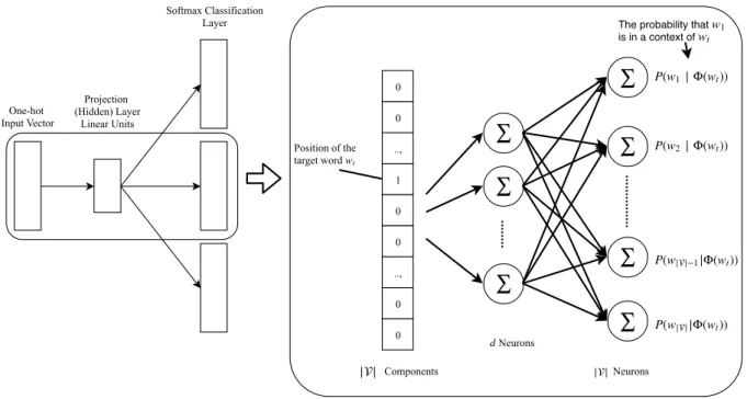
3. BACKGROUND 23 0 0 .., 1 0 0 .., 0 0 ∑ ∑ ∑ ∑ ∑ ∑ ∑ Position of the target word wt P(w1∣ Φ( ))wt P(w2∣ Φ( ))wt P(w||−1|Φ( ))wt P(w|||Φ( ))wt

The probability that is in a context of wtw1 || Components Neurons d ||Neurons Onehot Input Vector Projection (Hidden) Layer Linear Units Softmax Classification Layer

Figure 3.2: Architecture of the _SkipGram model

to project words into a latent continuous vector space that preserves the distributional semantics of words. That is, in the vector space, words that tend to co-occur within a context should be projected close to each other. In other words, we seek to learn a low-dimensional representation (the ‘Projection Layer’ of Fig. 3.2) of a target word that is capable of predicting its nearby or context words. To formally define the model, suppose we have a document corpus D = {Di : 1 ≤ i ≤ |D|}, and let Si be

the set of sentences in document Di, and S ∈ Si be a sentence specified as

a sequence of words:

S = w1, w2, . . . , w|S|, (3.7)

where each word wi is a sample from a vocabulary V. Consider the

functionsS(i) = wi that returns theith word in the sentenceS and function

(40)

3.3. SKIPGRAM 24 within a context size s:

context(S, wt, s) ={S(j) = wj : 1 ≤ t−s ≤j ≤ t+ s≤ |S|, j 6= t}

Then, for each target word S(t) = wt and a given context size s, the

SkipGram model maximizes the log probability of observing the set of

context words given the current target word:

max |S| X t=1 logP(context(S, wt, s)|wt) (3.8) max |S| X t=1 X wc∈context(S,wt,s) logP(wc|wt) (3.9)

As the goal is to embed words into a latent vector space, we condition on the current embedding of the target word Φ(wt) and rewrite Eq. 3.9 as

min− |S| X t=1 X wc∈context(S,wt,s) logP(wc|Φ(wt)) (3.10)

The technique employed by the _SkipGram model is also known as “learning by prediction” [3]. This is due to the optimization objective in Eq. 3.10 that is formulated as a prediction task of each context word given the embedding of a target word. The prediction task is normally handled as a softmax classification problem (hence the “Softmax Classification Layer” of Fig. 3.2) : P(wc|Φ(wt)) = exp(Φ(wc)T ·Φ(wt)) P w∈V exp(Φ(w)T ·Φ(wt)) (3.11)

That is, the model produces a conditional distribution P(wi|Φ(wt)) that

encodes the probability that each word wi ∈ V is a context word of a target

(41)

3. BACKGROUND 25 each encoding 1wc of the ground truth context word wc ∈ context(S, wt, s),

where 1wc ∈ {0,1}

V _{is a one-hot vector of} _w

c that has 1 for the component

associated with the position of wc and 0 everywhere as shown below.

1wc =         0 ... 1 ... 0        

However, training the _SkipGram model using the softmax formulation in Eq. 3.11 is very expensive due to the normalization constant that needs to be computed over all the vocabulary words w ∈ V. In this thesis we adopt the “negative sampling” technique [57] that characterizes a good model by its power to discriminate noise from the correct context words. Then, the computation of log P(wc|Φ(wt)) using the negative sampling

strategy is specified as:

P(wc|Φ(wt)) = logσ(Φ(wc),Φ(wt)) +neg(wt, `), (3.12)

whereσ is a sigmoid function, and the goal is to train a model that is capa-ble of effectively differentiating the proper context word wc of wt from the ` negative (noisy) samples wn drawn from some noise distribution N(wt)

of the target word wt. neg(wt, `) is the noise model, defined as:

neg(wt, `) =`·Ewn∼N(wt)[−logσ(Φ(wn),Φ(wt))] (3.13)

Equation 3.12 is equivalent to querying the model regarding its belief that

wc is a correct context word of wt as opposed to the negative samples wn.

Numerically, a good model should produce a small expected probability for the noise model and larger probability for the data model (the first term on the right-hand-side of Eq. 3.12).

(42)

3.4. AUTOENCODER 26 ∑ f ∑ f ∑ f ∑ f ∑ f ∑ f ∑ f ∑ f ∑ f ∑ f ∑ f ∑ f ∑ f ∑ f ∑ f ∑ f ∑ f ∑ f ∑ f ∑ f ∑ f ∑ f ∑ f ∑ f ∑ f ∑ f ∑ f

Figure 3.3: A standard architecture of an autoencoder. Each units of the feed-forward network constitutes a non-linear activation (f) of the linear transformationP

of its input. Finally, one can train the model using the entire document corpusDand an optimization algorithm like stochastic gradient descent (SGD). After a proper training – or after the model parameters (Φ) are tuned – we can use the embedding Φ(w) of each word w ∈ V for different kinds of natural language processing tasks.

3.4 AutoEncoder

An autoencoder (Fig. 3.3) is a feed-forward neural network that is com-monly used for an unsupervised machine learning. It has two components, which are called encoder and decoder. The encoder (the blue layers) is used to generate a compact and dense representation (the white layer) of a typically sparse and high-dimensional input data. The decoder (the green layers) tries to reconstruct the original input data from the compressed code. Informally, the objective is to train a model that learns a

(43)

high-3. BACKGROUND 27 quality compact representation of the input data capable to reconstruct the input data from the representation.

More formally, let I be the high-dimensional input data to the autoen-coder. Then we define, respectively, the encoder _enc and _dec in Eq. 3.14 and 3.15 as a composition of non-linear functions

Φ = _encL(HL_enc·_encL−1(. . .H2_enc ·_enc1(H1_enc ·I). . .)) (3.14)

I0 = _decL(HL_dec·_decL−1(. . .H2_dec·_dec1(H1_dec·Φ). . .)) (3.15)

whereL is the number of layers, Hl_enc andHl_dec are the weight matrices, and_encl and_decl are the non-linear functions, such assigmoidand tanh, of the lth layer of the encoder and decoder, respectively.

The training objective is commonly modeled as a minimization of the input reconstruction error

min||I−I0||2_F (3.16) Very often, due to the sparsity of I, the basic formulation is prone to learning to reconstruct the zeros, and a simple penalization trick is com-monly used to avoid this [77]. For this reason, the model is strongly penal-ized when it fails to reconstruct the non-zero elements and weakly penalpenal-ized for the zeros of the input data. This trick is achieved by introducing a term

S to the above equation as follows

min||(I−I0)⊗S||2_F (3.17) where ⊗ is the Hadamard product and S ∈ _Rn×n _{is associated with}

(44)

3.5. CONVOLUTIONAL NEURAL NETWORKS (CNN) 28

Sentence Embedding Layer

with multiple channels Convolutional Layer Max pooling overtime

Fully Connected Softmax Layer w₂ w₃ w_s w₁ Input Sentence

Figure 3.4: CNN model for sentence classification

The larger the value of µ, the stronger the penalty is on the reconstruction errors for the non-zero entries of I.

Usually, a regularization term or a dropout regularization technique is used to avoid over-fitting. Finally, one can train the model by optimizing either of the objectives in Eq. 3.16 or 3.17 depending on the sparsity of the input data I using algorithms such as stochastic gradient descent (SGD).

3.5 Convolutional Neural Networks (CNN)

Convolutional neural networks are widely used in different areas, such com-puter vision and NLP. In particular, they have proved to be highly effective in tasks such as object detection/recognition.

Generally, we can group them into two broad categories based on the type of input they process: 2-dimensional objects (such as images, video frames) and 1-dimensional objects (such as time-series, signals, and sen-tences in documents). In this thesis, we focus on the 1D variant that we have adapted to our problem.

(45)

sen-3. BACKGROUND 29 tence classification [42], whose architecture is depicted in Fig. 3.4.

The model takes a sentence S = w1, . . . , ws of length s as input. Each

sentence is embedded using a multi-channel embedding matrix. In the approach proposed by Kim [42], a fixed channel, based on pre-trained word embeddings and trainable channel that can be optimized with respect to the task-at-hand, for example sentence classification, have been used.

We illustrate now how a classification is carried out during inference time, supposing that all the model parameters have been already trained. Given an input test sentence St = w1, . . . , ws, its embedding matrix E =

[we1, . . . ,wes]T is constructed using the trained word embedding vectors

wei ∈ Rd of each word wi : i = 1, . . . , s. This corresponds to the sentence

embedding layer in Fig 3.4.

Then, in the convolutional layer the prediction task starts by applying a set of p filters on the cascade embedding matrix. That is, we apply p

filters (denoted by different colors) of different sizes on every possible slice of the input of the convolutional layer (the cascade embedding matrix). More formally,

φi,r = σ(hi·ejk +b) (3.18)

where the vector hi ∈ Rkd is the ith filter (kernel), b ∈ R is the bias, σ is an activation function, such as relu, k is the size of the ith filter,

φi,r is the feature value of the ith filter on the rth round convolution, and

ejk = ej ⊕. . .⊕ej+k ∈ Rkd is a concatenation of k rows of the matrix E,

starting from the jth row. Generally, the ith filter of size k is convolved

s−k+1 times, to give the feature mapsφ_i = [φi,1, . . . , φi,s−k+1]. φicaptures

patterns in high-level features, such as n–grams in language documents. Next, a max-pooling (or a max-pooling overtime) operation is applied over each feature map to sample from a specified pooling window, and the simplest technique is the one that draws from the entire feature vector,

(46)

3.5. CONVOLUTIONAL NEURAL NETWORKS (CNN) 30 best feature that is activated when a certain pattern in the input space is detected. The max-pooling output, more formally z = [φb₁, . . . ,φb_p], is

followed by a fully connected softmax classification layer. The vector zcan be viewed as the final set of features extracted for the current sentence, and it will be used to predict the sentence into one of the l ≥ 2 target classes Y = {yi : 1 ≤ i ≤ l}. This model was original proposed for binary

classification l = 2, henceforth we assume this setting.

The above description assumes that the model is trained; to perform the training, the optimization objective of the model is specified as the minimization of the misclassification error of the sentences. More formally, we adopt the standard binary cross-entropy objective function:

min−X

i

yilog(model(Si)) + (1−yi) log(1−model(Si)) (3.19)

Here,Si and yi ∈ {0,1}are the ith sentence and class label, respectively.

model is the proposed model that produces a probability distribution

(pre-diction) y for the given training sentence Si over the classes (1 and 0):

y = h·(z◦v) +b (3.20)

where v = [v1, . . . , vp] is a Bernoulli distribution used for dropout

regular-ization as proposed in [42], with vi ∈ {0,1}.

Ultimately, the model parameters [E, b,hi,h] are trained using the

(47)

Chapter 4 Network Representation Learning

with Structural Information

As we have discussed in the introduction, we approach the NRL task from two perspectives. This chapter is dedicated to the first one, where the network structure could be partially or completely known.

In general, the goal of a NRL task is to embed the nodes of the graph into a latent vector space in such a way that the most important properties of the network are preserved. Among such properties, for instance, those associated to the topology of the network are particularly important. For example, connectivity of nodes, the shape of their neighborhood, or their organization as a community; in general, the global proximity that each node has with rest of the nodes in the network. Preserving these proper-ties while embedding the nodes in the latent space enables one to perform different kinds of network analysis, such as link prediction and node clas-sification, in an efficient and effective way.

Thus, in order to obtain high-quality node embeddings that are going to be successful in the aforementioned tasks, we need to carefully investigate factors that govern nodes proximity or that could be attributed to their observed proximity.

In other words, first we should examine what factors have led users to

(48)

32 be located in a close proximity towards a given set of users and farther apart from others in a given information network. One of the most widely accepted theories from social science regarding the mechanism by which nodes might end up in a close proximity or create connection between them is homophily [56]. According to homophily, nodes prefer to connect with other nodes with whom they share similar properties, creating tightly connected communities. For example, in online social networks such as Facebook, users are more likely to befriend others with whom they share common characteristics (field of study, religion, race, schools, interests, etc.) rather than a random and unknown user [56, 88]. In addition, the homophily theory also highlights that ties between non-homogeneous nodes have less chance of surviving the test of time.

For this purpose, similar to [88], we associate a functional essence to every node in an information network, that characterize its intrinsic pref-erences. The following can be taken as examples of functional aspects of nodes in an information network:

• profile of a user in a social network

• attributes of an author in a scientific collaboration network

• functions of a protein in a protein interaction network

Secondly, we need to account for observed proximities, through the fac-tors that explain the observation itself, or through facfac-tors that could serve as a proxy for a certain level of observed proximity.

In summary, we account for three facets of an information network in learning embeddings of nodes:

• nodes functional essence

(49)

4. NRL WITH STRUCTURAL INFORMATION 33

• an indicator of the observed proximity

We assume that the nodes functional essence is the key factor that governs why nodes might prefer to be part of particular neighborhood in the network over the other. For example, assume that the interest

Θ = θ1, . . . , θτ over a set of τ topics corresponds to the functional essence

of nodes. Then, in line with homophily [56], nodes are likely to create connections or to be in a close proximity if they share strong interest in a set ϑ ⊆ Θ of topics.

Needless to say, it is necessary to account for the observed proximity. The third aspect is particularly important in cases where such proximity is only partially accessible or completely unaccessible. For example, the friendship and follower link structures of some users of social networks such as Facebook and Twitter is usually not accessible due to privacy constraints. In Wikipedia, the existing link structure between articles is incomplete due to the expensive manual effort involved to maintain it [62]. There is already a line of research that endeavors to improve the qual-ity of the links by exploiting Wikipedia clickstreams or human navigation traces [62, 72, 84], considering them as possible signals for a hidden proxim-ity between unlinked articles. For the case of social network users, processes like information diffusion events could play the role of the aforementioned signal.

In this study, attributes play the role of a functional essence of nodes and information diffusion events (cascades) that occur as a result of users interactions are used as indicators of an observed proximity. Intuitively, the main hypothesis behind the design of the proposed method in this chapter is as follows:

• if nodes have a strong attribute similarity, then they are likely to be in a close proximity;

(50)

4.1. SUMMARY OF CONTRIBUTIONS 34

• if nodes are in close proximity, then they are likely to have a strong interaction than random users farther away.

That is, we seek to develop an algorithm that preserves the topologi-cal proximity, attribute similarity and interaction history to learn a high-quality embeddings of nodes in an information network.

4.1 Summary of Contributions

In this study we propose a network representation learning algorithm based on topology, attributes and interaction histories. Earlier methods have fo-cused on topology alone, and recent approaches revisited NRL by incorpo-rating attributes. Although [82, 83] already noticed that diffusion events unveil interesting patterns about the topological orientation of nodes, ex-isting studies in NRL have overlooked this insight. In this chapter, we examine how we can incorporate information diffusion events into NRL.

This is particularly useful when part of the network topology is missing. We took inspiration from previous studies who examine the correlation between the network topology and the dynamics of information diffusion events. That is, we take advantage of the aforementioned studies to indi-rectly account for missing links in network structure by exploiting diffusion events that have propagated over the entire network, including the non-accessible part. This gives us an edge over most existing studies, that require the presence of the full network structure.

A naive approach towards designing a NRL that uses topology, at-tributes, and information diffusion sources could be to learn independent representations from each of these sources, to later merge the learned rep-resentations. However, this fails to account for the correlation that may exist between the representations [55]. For this reason, we propose a novel method that jointly learn embeddings from the aforementioned three facets

(51)

4. NRL WITH STRUCTURAL INFORMATION 35 of information networks.

We have carried out an extensive experimental evaluation of the pro-posed method using four real-world datasets, comparing it against state-of-the-art NRL techniques that are trained using the network structure only, across three kinds of network analysis problems.

4.2 Background and Problem

We use the graph definition proposed in Chapter 2, with uniform weights. That is, we consider a graphG = (V, E,W, a) where (i, j) ∈ E ⇒ W[i,j] = 1. In addition, we also use cascades without timestamps, that is, a cascade

C = [(u1, t1), . . . ,(u|C|, t|C|)] is transformed to strip(C) = [u1, . . . , u|C|].

The set of cascades transformed by striping time information are denoted by C0 = {strip(C) : C ∈ C}.

The last but not least information that we use are attributes; in this chapter, we consider textual attributes, that is, keywords associated to nodes. For a nodev ∈ V,a(v) corresponds to the set of keywords associated to v. Then we compute a new graph G0 = (V, E,W0) where W0 is a new weight matrix and each entry W[i,j]0 is defined as

W[i,j]0 = |a(i)∩a(j)|

|a(i)∪a(j)| (4.1)

In other words, the weights correspond to the Jaccard similarity between the set of keywords of node i and j. Note that W0 could be a very dense matrix if there is a popular attribute shared by all nodes. One can simply pruneG0to reduce these kinds of trivial similarities, however in our datasets no such attribute exist. In a follow-up study [66] we have tackled this issue by modeling attributes as a separate bipartite graph.

We take into account interaction histories that are recorded as a reaction of users to others’ post sorted according to their reaction time. This is

(52)

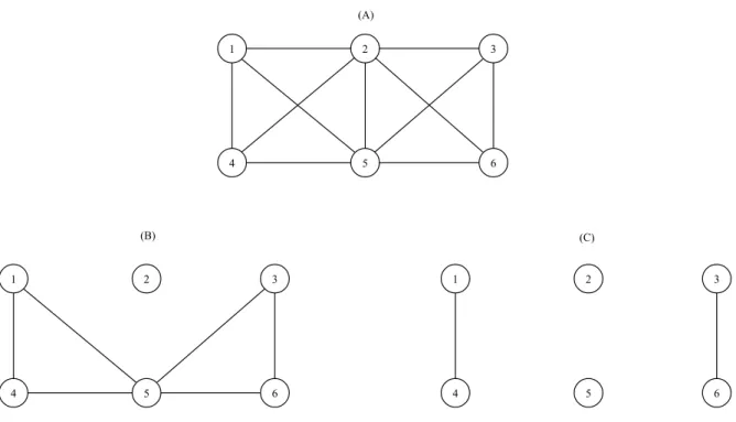
4.2. BACKGROUND AND PROBLEM 36 4 1 5 3 2 6 4 1 5 3 2 6 4 1 5 3 2 6 (A) (B) (C)

Figure 4.1: An example of a complete social network (A) and possible subgraphs (B) and (C) that could be crawled as a result of privacy settings of nodes. (B) If only node 2 have set its connection setting to private; and (C) if 3 have also decided to go private on its connections alongside 2.

exactly how we defined cascades in Chapter 2. Our assumption is that if a user generates a post, then it is more likely for another user in a close proximity to react to her post rather than a random user far away from the poster. In other words, we expect users in a close proximity to be involved in relatively similar cascades.

Suppose we have two disjoint communities, based on their interest in the Italian football club AC Milan and in Ethiopian politics. If a member of the AC Milan community posted a piece of content about the club, then its very likely for another member of this community to first react to the post than a member from the Ethiopian politics community. In general, we assume members of the Milan club community will have the tendency to appear in posts related to AC Milan and the Ethiopian community in posts related to the Ethiopian politics.

(53)

4. NRL WITH STRUCTURAL INFORMATION 37 Furthermore, as stated earlier, cascades will also give us the advantage in case we only have a partially observed topology of the network. We claim that they play a vital role when only part of the true proximity is accessible and no other side information is available, for example due to privacy constraints in social networks.

If we examine the sample social network in Fig. 4.1, the true connections might look like as the one in (A). However, as a result of users privacy setting an interested third party in need of access to the social network could end up crawling different kinds of subgraphs. For instance, if only node 2 sets its connection to private, the most complete subgraph one can crawl is the one in (B); if both nodes 2 and 3 also decide to make their connections private, then one could only crawl at best the subgraph in (C). Clearly, the node embedding learned from subgraphs (B) and (C) could be rather far from the optimal one, and hence it is imperative to incorporate additional sources of information that provide a clue regarding the missing links.

In social networks like in Fig. 4.1, cascades can be extracted from hash-tags, share and retweet activities, as shown in Table 4.1. We can exploit these to account for the missing links. Thus, even though one only has the subgraph in Fig 4.1 (B) or (C), a clever strategy could be devised to capitalize on possible patterns of interaction that could be associated with actual connections.

In this chapter, we only make a simple use of the cascades by combining them with sampled cascades. In Chapter 5 we shall demonstrate novel strategies to make a better use of the cascades for the NRL task. Now, we shall formally state the network representation learning problem that we seek to tackle in this chapter as follows:

Problem 1. Given a network G0 = (V, E,W0), a set of cascades C0 with no time information, a dimension d, we seek to learn a representation of

(54)

4.2. BACKGROUND AND PROBLEM 38

Hashtag Users sorted according to infection timestamps

#ht1 2,3,1,5,6 #ht2 3,4,2,1,5 #ht3 6,3,5,4,2 #ht4 1,6,5,3,4,2 #ht5 5,2,6,3 #ht6 1,3,4,5,2,6

Table 4.1: Cascades extracted from observed hashtag use of nodes of the social network in Fig. 4.1(A). A cascade is constructed by sorting nodes according to the time stamp that they have used a particular hashtag.

the network specified by Φ : V → _Rd_{, provided that Φ preserves nodes’}

• topological information (observed proximity);

• functional essence (preferred attributes);

• interaction pattern (tendency to reacting to others’ post).

Similar to [29], the aforementioned problem statement can be specified as solving the cost function

L = loss(_sim(u, v;W, a,C0),_sim(u, v; Φ)) (4.2)

Recall that the attribute information is now captured by the weights on the edges, and hence Eq. 4.2 can be reformulated as

L = loss(_sim(u, v;W0,C0),_sim(u, v; Φ)) (4.3)

In this study, L is materialized using cross-entropy as in Eq. 4.4. That is, the deviation of the similarity – _sim(u, v; Φ) between any pair of nodes

u, v ∈ V in the output or representation space Φ from their similarity –

sim(u, v;CI) in the input space CI.

L = − X

u,v∈V

(55)

4. NRL WITH STRUCTURAL INFORMATION 39 where the input space CI is a combination of the transformed cascades C0 and a new set of simulated cascades C00; more concretely,

CI = C0∪ C00

We provide the details of the technique used to sample simulated cas-cades C00 from W0 in Section 4.3.1.

4.3 The Learning Algorithm

As the weighted network captures both topological and attribute informa-tion, from now on it should be understood when we refer to the structure in this chapter, attributes are implicitly referred to. Therefore, we pro-pose an algorithm called_Mineral(Multi-modalNetworkRepresentation

Learning), inspired by an algorithm for language modeling called

Skip-Gram.

As we have discussed in Chapter 3, the _SkipGram model is used to project words into a latent vector space. The projection is done by ensuring that the latent vectors of words that have the tendency to frequently appear in the same context are embedded close to each other.

In our problem setting, we want to achieve a similar goal and seek to project nodes to a latent vector space where nodes that:

• are in a close proximity

• have similar functional essence

• have the same interaction patterns

should be embedded close to each other. _SkipGram, however, is special-ized for natural language documents. This introduces a challenge for our case, as the topological and functional essence of nodes are encoded in a