Network Representation Learning with Attributes and Heterogeneity

(1)

DEPARTMENT OF INFORMATION ENGINEERING AND COMPUTER SCIENCE ICT International Doctoral School

Network Representation Learning

with Attributes and

Heterogeneity

Nasrullah Sheikh

Advisor

Prof. Alberto Montresor

Universit`a degli Studi di Trento

(2)

(3)

Abstract

Network Representation Learning (NRL) aims at learning a low-dimensional latent representation of nodes in a graph while preserving the graph infor-mation. The learned representation enables to easily and efficiently perform various machine learning tasks. Graphs are often associated with diverse and rich information such as attributes that play an important role in the formation of the network. Thus, it is imperative to exploit this information to complement the structure information and learn a better representation. This requires designing effective models which jointly leverage structure and attribute information. In case of a heterogeneous network, NRL methods should preserve the different relation types.

Towards this goal, this thesis proposes two models to learn a represen-tation of attributed graphs and one model for learning represenrepresen-tation in a heterogeneous network. In general, our approach is based on appropriately modeling the relation between graphs and attributes on one hand, between heterogeneous nodes on the other, executing a large collection of random walks over such graphs, and then applying off-the-shelf learning techniques to the data obtained from the walks. All our contributions are evaluated against a large number of state-of-the-art algorithms, on several well-known datasets, obtaining better results.

Keywords

[Graph Embedding, Attributed and Heterogeneous Graphs, Unsupervised Learning]

(4)

(5)

Acknowledgment

Firstly, I would like to express my gratitude to my supervisor, Prof. Alberto Montresor for his advice and unflagging support over the course of the last three years. I am also grateful for his trust in me and for giving me the freedom to explore my research topic that helped me to accomplish this Ph.D. thesis.

Secondly, I would like to express my gratitude to my collaborators: Dr. Zekarias Kefato, Cristian Consonni, Dr. Amira Soliman, Dr. Leila Bhari, and Prof. Sarunas Girdzijauskas. I especially thank Zekarias Kefato for the extensive collaboration, ideas, and discussions. I thank Cristian Consonni, our Cricca research group member, for his help, insights, feedback and being there whenever needed. I would also like to thank my friends and colleagues at DISI, especially Dr. Kashif Ahmad, Dr. Maqsood Ahmad, Dr. Attaullah Buriro, Sudipan Saha, and Rajen Chatterjee for all scientific discussions and fun. Also, special thanks go to my friends in Kashmir: Dr. Firdous Ahmad, Zamir Ashraf, Attaullah, Dr. Mudasir, Umar, and Amjed. Further, I would like to thank ICT Secretariat and Ph.D. office, especially Andrea, Francesca and Roberta for their support in administrative matters. I would also like to thank Prof. Sarunas for hosting me at the Royal Institute of Technology, Stockholm (KTH) for an internship. It was a valuable and rewarding learning experience, and a privilege to work with Prof. Sarunas, Leila, and Amira.

Next, I would like to take the opportunity to thank Dr. Dawood A. Khan, who has been my mentor since my bachelor’s degree, for his invalu-able support and discussions.

Finally, I thank and express my gratitude to my parents, sisters, and brother for their continuous support and encouragement throughout my years of study.

(6)

(7)

5 Joint Learning on Attributed Graphs 35 5.1 Problem . . . 37 5.2 GAT2VEC Framework . . . 38 5.2.1 Network Generation . . . 38 5.2.2 Random Walks . . . 40 5.2.3 Representation Learning . . . 41 5.2.4 _gat2vec-wl . . . 44 5.3 Experiments . . . 45 5.3.1 Datasets . . . 45 5.3.2 Baseline Methods . . . 46

5.3.3 Experimental Setup & Parameter Settings . . . 47

5.3.4 Vertex Classification . . . 48

5.3.6 Qualitative Analysis . . . 53

5.3.7 Parameter Sensitivity . . . 57

6 A Simple Approach to Learn Representation on Attributed Graphs 61 6.1 Problem Definition . . . 63

6.2 Model . . . 63

6.3 Experiments . . . 66

(9)

6.3.2 Baselines . . . 67

6.3.3 Vertex Classification . . . 68

6.3.5 Network Reconstruction . . . 71

6.3.6 Algorithmic and Scalability Analysis . . . 73

7 Heterogeneous Information Network Representation Learn-ing 77 7.1 Problem definition . . . 78

7.2 Model . . . 78

7.2.1 Sequence Generation and Labeling . . . 79

7.2.2 _HetNet2Vec Model . . . 80 7.3 Experiments . . . 82 7.3.1 Datasets . . . 82 7.3.2 Baselines . . . 83 7.3.3 Experimental Setup . . . 83 7.3.4 Classification . . . 84

8 Predicting Virality of Cascades 87 8.1 Related work . . . 91

8.2 Model and definitions . . . 92

8.3 _cas2vec. . . 94

8.3.1 Preprocessing Cascades . . . 95

8.3.2 CNN model for cascade prediction . . . 98

8.4 Experiments and Results . . . 100

8.4.1 Datasets . . . 101

8.4.2 Baselines . . . 101

8.4.3 Evaluation Settings . . . 102

(10)

9 Conclusion 111

(11)

List of Tables

2.1 Notations used in the thesis . . . 14

5.1 Dataset Statistics . . . 46

5.2 Multi-class Classification on _dblp . . . 49

5.3 Multi-class Classification on _CiteSeer . . . 49

5.4 Multi-label Classification on _BlogCatalog . . . 50

5.5 _Macro-F1 score of classification (using labels) . . . 51

5.6 P(k) for Link Prediction on _dblp . . . 52

5.7 P(k) for Link Prediction on _BlogCatalog . . . 53

5.8 Nearest Neighbor Top 3 Results . . . 54

6.1 Dataset Statistics . . . 66

6.2 The Network Layer Structure for Enhanced Autoencoder . 68 6.3 Vertex Classification of _CiteSeer . . . 69

6.4 Vertex Classification of _cora . . . 69

6.5 Vertex Classification of _pubmed . . . 70

6.6 Vertex Classification of _wiki . . . 70

6.7 AUC and AP scores for Link Prediction . . . 71

6.8 Precision at K (P@K) for _CiteSeer dataset . . . 72

6.9 Precision at K (P@K) for _cora dataset . . . 72

6.10 Precision at K (P@K) for _pubmed dataset . . . 73

(12)

6.12 Computational Complexity and Scalability Analysis on

red-dit dataset (NA:out of memory) . . . 74

6.13 Running Time Analysis on _CiteSeer dataset (in seconds) 74

7.1 Dataset Statistics . . . 82 7.2 Multi-class Classification on Patents and Restaurants nodes 84

(13)

List of Figures

1.1 Overview of NRL Applications. . . 3

3.1 Architecture of _SkipGram model . . . 18

3.2 Architecture of Autoencoder model. . . 20

3.3 Architecture of Convolutional Neural Network . . . 22

5.1 An example of a partially attributed graph. . . 36

5.2 A graph depicting the structural relationships between ver-tices. . . 38

5.3 A bipartite graph between content nodes and attributes. . 39

5.4 The Architecture of _gat2vec. . . 41

5.5 2-D t-SNE Projection of _CiteSeer Dataset . . . 56

5.6 Ga Parameter Sensitivity on: (a) Number of Walks(γa), (b) Walk Length(λa) . . . 58

5.7 Ga Joint Parameter Sensitivity on: (a) Number of Walks(γa), (b) Walk Length(λa) . . . 59

5.8 Sparsity of Attributed Graph Ga . . . 59

5.9 Effect of parameter-th . . . 60

6.1 The architecture of our proposed _Sage2Vec model . . . . 64

7.1 The adopted 1D-CNN Architecture for Representation Learn-ing in _HIN . . . 80

(14)

8.1 Examples of two recent hashtag campaigns. (A) The tweet-ing frequency of each hashtag; #metoo achieved more spread compared to #gamergate. (B) The network properties of the participating nodes in each hashtag in terms of average number of followers; the nodes engaged in the first 12 hours

almost achieve similar reachability in both hashtags. . . 88 8.2 Two slices of size 2 hours, applied to the user coverage

distri-bution of a viral hashtag (#thingsigetalot) and non-viral hashtag (#bored), which have reached 13711 and 43 users

in an observation window size of 4 hours. . . 94 8.3 The distribution of the user coverages for the viral and

non-viral classes. The user coverage distribution is computed at observation time to as |C(to)| and virality is computed at

prediction time to + ∆. A cascade is viral if |C(to + ∆)| ≥

1,000 and not-viral if |C(to + ∆)| ≤500 . . . 97

8.4 The CNN model adopted for cascade prediction . . . 98 8.5 Virality prediction results for both of our datasets. For

Twitter, filter sizes = 3, 5, 7 and for each filter we have 16 of them. For Weibo, filter sizes = 2, 4, 5, 7 and for each filter we have 64 of them. For both datasets, the embedding sizedis 128, the number of units in the fully connected layer

is 32, and the number of slices is 40. . . 102 8.6 Evaluation results of early prediction experiments for the

Twitter and Weibo datasets. The same hyper-parameter

values as Fig. 8.5 is used . . . 105 8.7 Break-out coverage for k = 100 and k = 200 for the Twitter

dataset. . . 107 8.8 Break-out coverage for k = 10 and k = 20 for the Weibo

(15)

8.9 Effect of the number of slices on virality prediction at to = 1

hour and ∆ = 12 hours. . . 108 8.10 Effect of sequence length on running time. . . 108 8.11 Effect of seq. length on virality prediction. . . 109

(16)

(17)

Chapter 1 Introduction

Graphs are ubiquitous: a large number of systems from diverse domains (social, biological, technological) can be represented as graphs. Examples include protein-protein networks, molecular structures, the World Wide Web, Online Social Network (OSN), power grids and communication net-works. The entities present in the system are represented as nodes and the structural relationships between them are represented as edges. For example, in the case of an OSN, the entities are the users, and relation-ships such as friendship or follower-followee are the edges connecting them. Representing a system as a graph allows to exploit the expressive power of graphs and to obtain various insights about the system, such as pattern discovery.

Analyzing graphs through machine learning has a variety of applica-tion across different domains; for example, annotating proteins by role in protein-protein interaction networks [1, 2], classification of users and rec-ommendation of new friends in online social networks [3–6], information diffusion in social networks [7, 8].

The performance of these applications largely depends on the features that are used to model the graph. A simple feature representation is an adjacency matrix that only captures the neighborhood information.

(18)

Un-2 fortunately, this representation does not encode the complex structural properties of the network such as higher-order proximities, which helps in the classification task. Moreover, the resulting representation is sparse and brings with it the curse of dimensionality; this deteriorates the per-formance of machine learning tasks. Furthermore, since graphs of interest tend to be really large, this representation makes machine learning tasks computationally expensive, hence not scalable to large graphs.

Earlier handcrafted features were used in machine learning tasks. These features include node degree, clustering coefficient, common neighbors, etc. The extraction of these features is time-consuming and expensive, in addi-tion to their inflexibility to adjustment during learning.

To overcome these bottlenecks, Network Representation Learning (NRL) approaches have been proposed to encode and preserve the structural prop-erties of a graph in a low-dimensional latent vector representation of nodes which is much smaller than the cardinality of the graph. NRL methods are built on a basic hypothesis: “birds of same feather flock together”, that is, similar vertices in the graph should be close to each other in the rep-resentation space. Following this, if two vertices are directly connected in the graph, the distance in the embedding space between their latent vec-tor representation should be small. The learned representation makes it easy to perform various network analysis tasks, and machine learning tasks can also be directly applied by taking these learned embeddings as feature inputs as shown in Figure 1.1.

The success of NRL methods depends on their ability to exploit the dif-ferent sources of information present in the graphs. The simplest and com-mon source is the structural information, i.e the connectivity of nodes in the graph. The methods which use structural information focus on preserving the structural proximities of the graph. Graphs, however, are often asso-ciated with additional information such as attributes. The co-occurrence

(19)

3 CHAPTER 1. INTRODUCTION 1 3 4 2 6 5 7 8 b a c b e b a c d e 9 d e Vertices Attributes Representation Graph [0.25, 1.8, ... , 0.03] [-0.5, 0.08, ... , -0.1] [0.17, 2.03, ... , -.23] ... Node Classiﬁcation Recommendation Network Reconstruction Community Detection Tasks Clustering Link Prediction NRL Nearest Neighbor

Figure 1.1: Overview of NRL Applications.

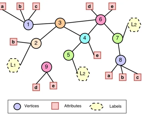
of attributes between nodes reinforces similarities between them, and thus alone structural proximities are not sufficient to capture the entire spec-trum of similarities. For example, in the attributed graph shown in Fig-ure 1.1, attributes are invaluable in cases where structural information is missing, or when structurally unrelated vertices have high attribute sim-ilarity. Vertex 9 is disconnected, but with the aid of attributes, it can have a representation similar to vertex 6. In the same way, vertices 1 and 8 are structurally far away from each other, but they have similar at-tributes. Therefore, the proximities in a graph can also be defined by their similarities in their attributes. By taking attribute proximities into consid-eration, representations of 1 and 8 will be close to each other. Moreover, the two sources of information can complement each other in learning, es-pecially when our knowledge of one of them is only partial. Thus, it is of paramount importance to consider attribute similarities in order to learn precise embeddings. The challenges are compounded when such additional information is included, as the NRL methods have to encode and preserve both the structural and attribute proximities.

(20)

1.1. MACHINE LEARNING TASKS FOR EVALUATION 4

1.1 Machine Learning Tasks For Evaluation

We focused mainly on three machine learning tasks for the evaluation of our proposed approach. We briefly describe them in this section.

1.1.1 Node Classification

The classification task assigns a class label from a given set of classes to an unlabeled data based on a training dataset. When only two classes are possible, it is called binary classification. If there are more than two classes and each data point can have only one label, the task is called as

multi-class classification whereas, when data instances can have more than one class label it is called as multi-label classification.

In this thesis, we leverage the structural and attribute information to learn a representation to effectively tackle node classification. We learn a representation and use it as feature vectors for the classifier. We use both multi-class and multi-label classification for node classification task depending on the dataset.

1.1.2 Link Prediction

The aim of link prediction is to predict the missing links or possible new connections based on the observed connections. For example, given an OSN, knowing the current connections (friendships), we want to predict the probability of an edge between two unconnected users; hence, we can recommend these two users to each other based on such probability. Other examples are academic networks such as co-author networks, in which it is interesting to know which two authors are highly likely to collaborate in the future. In the above examples, not only the connectivity, but also the attributes (e.g “likes” in an OSN and fields of interest in an academic network) may play a vital role in future connections.

(21)

5 CHAPTER 1. INTRODUCTION

In this thesis, to model predictions of future connections, we extract a residual graph by removing some edges and then learn a representation through our model. The removed edges serve as ground truth for evalua-tion, and the existence of an edge is computed from learned embeddings.

1.1.3 Nearest Neighbor Search

Nearest Neighbor (NN) is the proximity search algorithm which finds k -nearest data-points to a query data-point. In an attributed graph, the near-est nodes to a query node are those which are in close proximity, both in structure and attributes. For example, if two nodes,B{z1, z2, z3}, C{z4, z5, z6} are connected directly to A{z1, z2, z3}, it is obvious that node B is closer to A than node C, because node A has a higher attribute similarity to B

rather than C.

In this work, we apply representation learning on an attributed graph in a way that unifies structural proximity and attribute proximity in a single d-dimensional vector space; thus, the similarity between any two given nodes can be computed by using a distance metric.

1.2 Thesis Overview and Contribution

The focus of this thesis is on network representation learning of attributed and heterogeneous graphs, building models that learn a better representa-tion. We focus on three problem domains: attributed graph representation learning, heterogeneous graph representation learning, and cascade virality prediction.

For the sake of consistent reading of the thesis, Chapter 2 introduces some preliminaries and notations. Chapter 3 provides a detailed study of some models on which the proposed solutions are built. The state-of-the-art covering the major aspects of representation learning is discussed in

(22)

1.2. THESIS OVERVIEW AND CONTRIBUTION 6

Chapter 4. The two models of Attributed Graph Embedding is discussed in Chapter 5 and 6. Chapter 7 presents a model for Heterogeneous Graph Embedding. A virality prediction model in OSN is presented in Chapter 8. Finally, we conclude this dissertation in Chapter 9. The contributions of this dissertation are the following:

1.2.1 Chapter 5: Joint Learning on Attributed Graphs

To learn a better representation, the two modalities (structure and at-tributes) need to be taken into account jointly to learn a representation, as they complement each other. We observe that a node has two texts: a structural context and an attribute context. The structural con-text describes the nodes which are similar to a given node in terms of edge connections, whereas the attribute context of a node describes the nodes which are semantically similar to a given node. Therefore, a representation learning model needs to jointly optimize on these two distributions.

We propose _gat2vec, an early fusion model that jointly learns a rep-resentation from structural contexts and attribute contexts. To obtain contexts from an attributed graph, we build two graphs: the structural one given by the nodes and their connections, and bipartite one, which connects vertices with the attributes. We employ random walks on both structural graph and bipartite graph to generate structural contexts and attribute contexts respectively. We then use the_SkipGrammodel to learn a representation from both contexts.

Through experimental evaluation, we showed that a joint learning model learns precise embeddings that preserve network proximities, through ver-tex classification, link prediction, and nearest neighbor results.

Publication Nasrullah Sheikh, Zekarias Kefato, and Alberto Montre-sor. _gat2vec: Representation learning for attributed graphs. Computing 101(3):187-209. Springer, 2019.

(23)

1.2.2 Chapter 6: A Simple Approach to Learn Representation on Attributed Graphs

As the network structure is highly non-linear and sparse, shallow learning architectures learn poor representations. Furthermore, learning is even more challenging when attributed graphs are taken into considerations, as attributes themselves bring their own sparsity and non-linearity. This problem can be solved by designing deep neural networks which handle non-linearity and sparsity in both structure and attributes, but this adds more complexity. To model the proximities in an attributed graph, existing proposed methods use computationally expensive pre-processing–such as sampling–which limits their scalability.

We propose a simple enhanced autoencoder model (_Sage2Vec) that handles the non-linearity and sparsity of both the structure and attributes, without the need of computationally expensive preprocessing. We train the model on the network structure and optimize it on both the vertex neighborhood and the attributes. The experimental evaluation on vertex classification, link prediction, and network reconstruction tasks shows that our simple model is good at handling non-linearity and sparsity, while preserving the proximities.

Publication Nasrullah Sheikh, Zekarias T. Kefato, and Alberto Mon-tresor. A Simple Approach to Attributed Graph Embedding via Enhanced Autoencoder. Submitted to Data Science and Advanced Analytics 2019.

1.2.3 Chapter 7: Heterogeneous Information Network Repre-sentation Learning

A heterogeneous network has multiple types of nodes and relationships, and each relationship has different semantics. The homogeneous network embedding methods cannot be applied to heterogeneous networks because

(24)

1.2. THESIS OVERVIEW AND CONTRIBUTION 8

their sampling methods, such as random walks, are based on a homoge-neous distribution of nodes and edges. Therefore, network representation learning approaches need to explicitly take care of different node types and relationships while sampling, such that the learned embeddings preserve the network properties.

In this thesis, we propose a relation-specific short random walk for gen-erating sequences which represent the contextual relationships between nodes. We obtain a corpus of sequences by performing multiple random walks on each relation. The corpus of a sequence is analogous to sentences of a document, and we train a 1D-CNN for learning an embedding of nodes. The preliminary results show that our proposed approach_HetNet2Vec performs well and there is a lot of space for improvement.

Publication Nasrullah Sheikh, Zekarias T. Kefato, and Alberto Mon-tresor. Semi-supervised heterogeneous information network embedding for node classification using 1D-CNN. In Proc. of the Fifth International Con-ference on Social Networks Analysis, Management and Security (SNAMS 2018), pages 177–181. IEEE, October 2018.

1.2.4 Chapter 8: Predicting Virality of Cascades

This chapter slightly deviates from the main thesis topic as it deals with cascade virality prediction. The chapter is presented to show that the network agnostic approaches can be developed for drawing insights from a network system.

In Online Social Networks, it is common to see posts or tweets that start from a few sources and then suddenly spread like a wildfire. Just to mention a recent example, the post celebrating the landing of the Falcon-Heavy rocket sent from the SpaceX Twitter account on February 6th, 2018,

(25)

has been retweeted more than 75k times within the same day of posting1. Such diffusion events are calledviral cascades. Predicting cascades virality is vital for different applications, for example to forecast trends and rumor break-outs [8]. However, it is challenging to effectively predict the virality of such kinds of events as early as possible, especially when little supporting information is available. Many research works have dedicated effort and attention to the prediction of content popularity with the focus of achieving good predictions in the shortest possible time, with the least information possible about the underlying network structure.

The diffusion of content on OSN happens through the underlying user connectivity graph, which plays an important role in determining the vi-rality of content. Therefore, for the prediction of vivi-rality, it is necessary to take the properties of the underlying graph into account along with the cascade of information diffusion. The major challenge is to obtain the un-derlying social graph due to privacy concerns and the cost of mining such data. Thus, it is imperative to design virality prediction algorithms that are network oblivious but at the same time effective in prediction.

We propose _cas2vec, a network-agnostic approach that uses explicit information available in cascades with the premise that the reaction time between two events is a sufficient indicator to predict the virality. The reaction time in cascades enables us to model it as a time series where each element is a discretized reaction time. Noticing that the distribution of reaction time is similar to the distribution of words in a language, we have applied CNN model from Natural Language Processing (NLP) to train our prediction model. The results from experimental evaluation testify our premise of modeling cascades as a time series and our model performs well in predicting the virality.

The organization of this chapter is as follows: Section 8.1 describes the

1

(26)

1.3. PUBLICATION LIST 10

state-of-the-art, while Section 8.2 provides some definitions. The model for virality prediction is described in Section 8.3, followed by experimental setup and evaluation in Section 8.4.

Publication Zekarias T. Kefato, Nasrullah Sheikh, Leila Bahri, Amira Soliman, Alberto Montresor, and Sarunas Girdzijauskas. CAS2VEC: network-agnostic cascade prediction in online social networks. In Proc. of the 5th International Conference on Social Networks Analysis, Management and Security (SNAMS 2018), pages 72–79. IEEE, October 2018 Best Paper Award.

1.3 Publication List

The publications which contributed to this thesis are the following:

1. Nasrullah Sheikh, Zekarias Kefato, and Alberto Montresor. “gat2vec - Representation Learning for Attributed Graphs”. In Journal of Com-puting. Springer, May 2018.

2. Nasrullah Sheikh, Zekarias T. Kefato, and Alberto Montresor. A Sim-ple Approach to Attributed Graph Embedding via Enhanced Autoen-coder Data Science and Advanced Analytics 2019 (under review)

3. Nasrullah Sheikh, Zekarias T. Kefato, and Alberto Montresor. “Semi-Supervised Heterogeneous Information Network Embedding for Node Classification using 1D-CNN”. In Proc. of the First International Workshop on Deep and Transfer Learning (collocated with SNAM). DTL ’18. Oct. 2018.

4. Zekarias T. Kefato, Nasrullah Sheikh, et al. “CAS2VEC: Network Agnostic Cascade Prediction in Online Social Networks”. In Proc. of

(27)

the Fifth International Conference on Social Network Analysis, Man-agement and Security. SNAM’18 Oct. 2018. Best Paper Award.

Other Contributions During the research period, I collaborated on other research works which resulted in the following publications:

1. Zekarias T. Kefato, Nasrullah Sheikh, and Alberto Montresor. “RE-FINE: Representation Learning from Diffusion Events”. In Proc. of the Fourth International Conference on Machine Learning, Optimiza-tion and Data Science. LOD’18. Sept. 2018

2. Zekarias T. Kefato, Nasrullah Sheikh et al. “CaTS: Network Agnostic Virality Prediction Model to Aid Rumour Detection”. In Proc. of the Second International Workshop on Rumours and Deception in Social Media (Collocated with CIKM). RDSM’18. Oct. 2018.

3. Zekarias T. Kefato, Nasrullah Sheikh, and Alberto Montresor. “MIN-ERAL: Multi-modal Network Representation Learning”. In Proc. of the Third International Conference on Machine Learning, Optimiza-tion and Big Data.MOD’17. ACM, Sept. 2017.

4. Zekarias T. Kefato, Nasrullah Sheikh, and Alberto Montresor. “Deep-Infer: Diffusion Network Inference through Representation Learning”. In Proc. of the 13th International Workshop on Mining and Learning With Graphs. MLG’17. ACM, Aug. 2017.

(28)

(29)

Chapter 2 Preliminaries

In this chapter, we introduce the various notations and definitions used in this thesis.

2.1 Notations

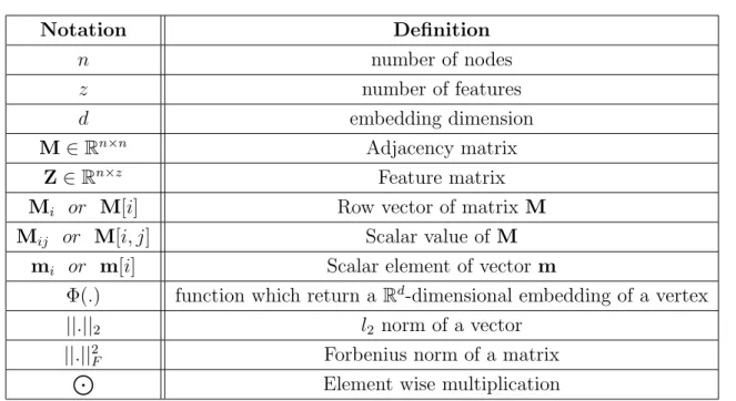
Scalars are represented with lower case letters, sets with uppercase letters. Matrices and vectors are denoted with uppercase and lowercase boldface letters, respectively. The main symbols used in this thesis are given in Table 2.1.

2.2 Definitions

Definition 1. [Attributed Graph] Let G= (V, E,M,Z) be an attributed graph, where V is a set of n nodes, E a set of edges, Mn×n is the adja-cency matrix representation of the edges and Zn×z is the feature matrix representing z features associated with nodes.

Let Mi be the ith row vector and let Mij 6= 0 if there is an edge between

the ith and jth vertex. Let Zi be the feature vector of the ith vertex, where

(30)

2.2. DEFINITIONS 14 Notation Definition n number of nodes z number of features d embedding dimension M∈_Rn×n _{Adjacency matrix} Z ∈_Rn×z _{Feature matrix}

Mi or M[i] Row vector of matrix M

Mij or M[i, j] Scalar value of M

mi or m[i] Scalar element of vector m

Φ(.) function which return a _Rd_{-dimensional embedding of a vertex}

||.||2 l2 norm of a vector ||.||2

F Forbenius norm of a matrix

J

Element wise multiplication Table 2.1: Notations used in the thesis

For an unweighted graph, Mij = 1 in case there is an edge between

vertex i and j. In case of a weighted graph, Mij 6= 0 is the weight of an

edge between vertex i and j. If there is no edge, then Mij = 0 for both

types of graphs.

Definition 2 (First-Order Proximity[9]). The first-order proximity be-tween two nodes i and j is determined by |Mij| > 0, that is, these two

vertices are directly connected. It is also called as local pairwise proximity.

Definition 3 (Second-Order Proximity[9]). The second-order proxim-ity between ith and jth node of graph G is determined by the similarity between their common neighbors i.e. similarity between Mi and Mj.

Definition 4 (Higher-Order Proximity). Let Mˆ be a one-step transi-tion probability of M and M0 = ˆM+ ˆM2+· · ·+ ˆMk is the k-step transition probability between each pair of vertex. The high-order proximity between

ith and jth is determined by the similarity between M0i and M0j.

Definition 5 (Context). Let V = {v1, v2,· · · , vn} be the set of words

(31)

15 CHAPTER 2. PRELIMINARIES

context window. The context of a word v is c words before and after it, i.e

{vi−k,· · · , vi−1, vi+1,· · ·vik}.

Definition 6 (Heterogeneous Graph). A Heterogeneous Information Network (HIN) is a graph Gh = (V, E, f, g), where V is the set of nodes,

E ⊆ V × V is the set of edges, f : V → TV is a function mapping each

node v ∈ V to one node type in TV, and g :E → TE is a function mapping

each edge e ∈ E to one edge type in TE.

2.3 Evaluation Metrics

The embedding methods are evaluated using different machine learning tasks such as node classification and link prediction. In this section, we will give brief details about the metrics used to evaluate the tasks.

Definition 7. Precision is the fraction of samples correctly classified as positive over all positively classified samples. Mathematically, it is defined below:

pr = T p

T p+F p (2.1)

Definition 8. Recall is the fraction of samples correctly classified as pos-itive over all correct classifications as described below:

rc = T p

T p+ F n (2.2)

where in Equation 2.1 and 2.2, T p, F p, and F n are true-positives, false-positives, and false-negatives respectively.

For an effective evaluation of the model, both precision and recall are necessary. Since they are antagonistic to each other, therefore, maximizing the combination of them gives an optimal solution, called _F1-Score. It is computed as:

F1-Score = 2· pr ×rc

(32)

2.3. EVALUATION METRICS 16

The general case of F-measure is given as:

Fβ-score = (1 +β2)·

pr ×rc

β2 _×₍_pr ₊_rc₎ (2.4) In the case of multiclass and multilabel classification _F1-Score is aver-aged due to the presence of independent classes. _Micro-F1 and

Macro-F1 are two statistics calculated in this case. Macro-F1 gives the equal

weight to each class and the metrics are calculated for each class. Let pr(.)

and rc(.) be the functions that return theprecision andrecall for each class

respectively. The average precision (pravg) and recall (rcavg) are calculated

as: pravg = P c∈C pr(c) |C| rcavg = P c∈Crc(c) |C| where C is the set of classes.

Macro-F1 is given is harmonic mean of average precision and recall

calculated as:

Macro-F1 = 2× pravg ×rcavg pravg +rcavg

(2.5)

In _Micro-F1 average, we sum the scores of different class and calcu-late the overall precision and recall. Let tps(.), f ps(.), and f ns(.) be the

functions that return the true positives, false positives and false negatives for a given class, respectively. _Micro-F1 is calculated as:

pra = X c∈C tps(c) tps(c) +f ps(c) (2.6) rca = X c∈C tps(c) tps(c) +f ns(c) (2.7)

Micro-F1 is the harmonic mean of pra and rca as given below:

Micro-F1 = 2× pr_pra ×rca

a+rca

(33)

Chapter 3 Background

This chapter provides the necessary and sufficient details of the methods on which the work in the thesis is built upon. The sections 3.1, 3.2, and 3.3 are the foundations for the solutions proposed for Chapters 5, 6, 7 and 8.

3.1 SkipGram

Representing the words of text in a continuous vector representation is a very crucial problem in Natural Language Processing (NLP), as they significantly simplify and improve NLP applications. The continuous vec-tor representation preserves the semantic meaning of words and overcomes sparsity. Various models that have been proposed earlier were limited by their lack of scalability i.e., they were significantly computationally expen-sive in training [10–12]. These model were trained on small corpora, thus the learned representations were of low quality. Mikolov et al. proposed a distributed word representation learning model called _Word2Vec that is scalable and preserves the semantic meanings of the words [13]. The preservation of the semantic properties is demonstrated through various examples, such as the vectors of synonyms of a word tend to be close in representation space. Another fascinating example is from the analogy,

(34)

3.1. SKIPGRAM 18

algebraic operation as well: Φ(queen)−Φ(woman) + Φ(man) ≈ Φ(king), where Φ(.) returns the embedding of the given word.

.... ... ... . .... ... ... . . . . .... ... . . .... .. .... ... . . .... .. Output Layer n Hidden Layer 0 0 0 . . . 0 . . 0 Input Layer Wn×d Wd×n′ W′ d×n Wd×n′ y1j y2j ycj xi d

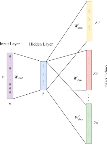
Figure 3.1: Architecture of SkipGram model

Word2Vecproposed two architectures, Continuous Bag-of-words (CBOW)

and _SkipGramfor learning representation of words. In the CBOW model, the occurrence of a word is predicted from a given set of context words. The model is trained through a log-linear classifier which tries to correctly predict a middle word from a set of context words. The experiments show that this model does not perform better than _SkipGram. Therefore, we skip the details of this model and we focus on _SkipGram. The architec-ture of _SkipGram is shown in Figure 3.1. Let V = {v1, v2,· · · , vn} be

the set of words (vocabulary) of size n, C be the set of all contexts, and

(35)

19 CHAPTER 3. BACKGROUND

are all contexts associated with it. For a given word v and its contexts c, the _SkipGram model considers the conditional probabilities p(c|v). The probability is calculated using soft-max as given below:

p(c|v) = e Φ(c).Φ(v) P c0∈C eΦ(c 0 ).Φ(v) (3.1)

The goal is find a parameter θ such that probability p(c|v;θ) is maxi-mized as: arg max θ Y (c,v)∈T p(c|v;θ) (3.2)

Applying the logarithm we get:

arg max θ Y (c,v)∈T p(c|v;θ) = X (c,v)∈T  log e Φ(c).Φ(v) ₋ log X c0∈C eΦ(c 0 ).Φ(v)   (3.3)

Since summation over all other contexts c0 in the above equation makes it computationally expensive as there can be thousand of other contexts, the soft-max is replaced with the hierarchical softmax.

Hierarchical softmax is an approximation to softmax proposed by Morin and Bengio [14]. It is a complete binary tree where the words are the leaf nodes and the root is the given word. Thus, the prediction task is to find a path that maximizes the probability for the given word.

3.2 Autoencoder

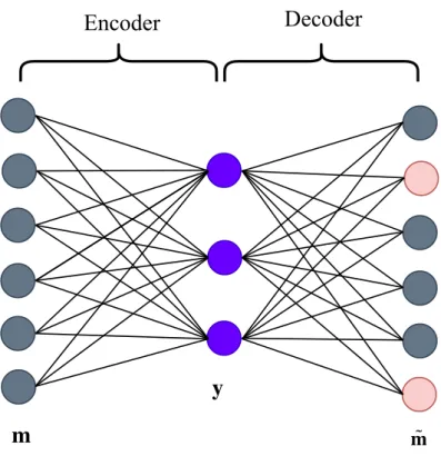
An autoencoder is an unsupervised neural network model that learns a representation of the input data. Traditionally, autoencoders have been used for dimensionality reduction and feature learning [15–17]; due to re-cent advancements in neural networks, they are also used in generative models. An autoencoder consists of two parts: an encoder function which

(36)

3.2. AUTOENCODER 20

compresses the input data y = f(m) and a decoder function, ˜m = g(y) tries to reconstruct the input as close as possible. m is an input vector, y is the latent representation, and ˜m is the reconstruction. In other words, the autoencoder tries to learn an identity function such that m ≈m. The˜ autoencoder functions are constrained so that they are not able to copy the input exactly. This is achieved by forcing the autoencoder to prioritize to learn only useful properties of the input which is achieved by constraining y to a smaller dimension than m. A possible architecture of an autoen-coder with one hidden layer is shown in Figure 3.2. The two red circles in the decoder signify the error in reconstruction. Mathematically, encoders and decoders are described by Equation 3.4 and 3.5, respectively.

m

y

Encoder Decoder

m̃

(37)

y = f(W.m+b) (3.4) ˜

m = g( ˜W.y+ b) (3.5)

Here W,W˜ are weight matrices for encoder and decoder respectively and

b is the bias term.

The learning objective of an one-layer autoencoder is described by the minimizing loss function as given under:

L = E(m,m)˜ , (3.6)

where E is the loss function that penalizes ˜m for being dissimilar to m. Mean Square Error (MSE) and binary cross entropy are some examples of loss functions used. The MSE loss is given as below:

L = km−mk˜ 2₂ (3.7)

In general, for a deep autoencoder with L layers and m as input, the encoder function can be described as:

y(1) = f(W(1)m+b(1))

y(l) = f(W(l)y(l−1) +b(l)), l = 2,· · · , L

(3.8)

yl is the latent representation of m at the lth layer; L is the number of layers; W(l) is the weight matrix and b(l) is the bias at the lth layer. The decoder is the reverse of the encoder; thus, it takes y(l) as input and pro-duces the reconstruction m.˜

An autoencoder learns an embedding in the same subspace as PCA when the decoder function g is linear and the error function is MSE. In case, f and g are both non-linear functions; thus, learned embeddings are nonlinear generalizations of PCA.

(38)

3.3. CONVOLUTIONAL NEURAL NETWORK 22

3.3 Convolutional Neural Network

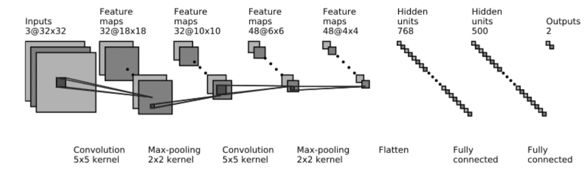
Convolutional Neural Network is a deep neural network which operate on grid-like data such as images and sequences [18]. CNN extracts local features by exploiting shift-invariance, local connectivity, and composition-ality of the data. A CNN consists of three components: the convolutional layer, the pooling layer, and the fully-connected layer. An example archi-tecture1 of CNN is given in Figure 3.3. The architecture takes an image with three channels (RGB) as input and applies two convolutions and max-pooling operations. Feature maps 48@4x4 Feature maps 48@6x6 Feature maps 32@10x10 Feature maps 32@18x18 Inputs 3@32x32 Convolution

5x5 kernel Max-pooling2x2 kernel Convolution5x5 kernel Max-pooling2x2 kernel

Hidden units 768 Hidden units 500 Outputs2 Flatten Fully

connected Fullyconnected

Figure 3.3: Architecture of Convolutional Neural Network

Convolutional Layer This layer applies the convolution operation to the input; the output from the convolution is called feature map. The convo-lution operation is performed through filters, also referred as kernels; the areas on which convolution is applied is called receptive field. Kernels en-able the CNN to extract high level features which are shift and positional invariant. Let I be an input 3-channel(RBG) image of size n×n; kernel K has a size h×w and the depth of the filter is equal to number of channels.

1_{Generated using}

(39)

The i, j-th feature from a receptive field is computed as as:

C[i, j] = X

p

X

q

I[i−p, j −q]·K[p, q] (3.9)

The convolution performs an element-wise multiplication with the input. The filter is slid horizontally and vertically along the image, and the slide is controlled by parameter s. In Figure 3.3, the first convolution layer has a filter of 5×5×3, and s = 1, thereby producing a feature map of 28×28. To preserve the spatial dimensions, a number of filters are applied. In the example, we have 32 filters producing 32 feature maps; on each of them, an activation function is applied. The weights of filters are trained through the backpropagation algorithm.

Pooling is a downsampling process to further reduce the size of the input by computing a summary statistic of nearby points. Pooling can be done through various methods such asmax-pooling andaverage-pooling. In max-pooling, a maximum value is returned from a patch of the image and the rest are discarded. In average-pooling, an average value is returned from a patch.

Fully Connected Layer The output from the pooling is flattened and fetched to a fully connected layer component. The number of FC-layers vary de-pending on the complexity of the data and the model. The result from the FC-layer can be used for various machine learning tasks such as classifica-tion.

(40)

(41)

Chapter 4 State-of-the-art

The objective of this chapter is to provide an overall overview of the meth-ods designed to learn a representation of nodes in a graph. This chapter will outline an evolution of techniques–from simple to complex–exploiting different modalities. Broadly, we classify the NRL methods in two cate-gories: homogeneous and heterogeneous network embedding, depending on the type of nodes and relationships present in a graph. In homogeneous NRL methods, the nodes and the edges are of a single type, whereas in the case of heterogeneous NRL methods nodes and edges are of different types.

4.1 Homogeneous Network Embedding

In this section, we describe the various methods proposed to learn a repre-sentation. These methods use various different sources of information for learning. Broadly speaking, homogeneous network embedding methods are divided into two groups: plain network embedding and attributed network embedding. To learn a representation, the former methods use only the structure of the network, whereas the latter methods use both the network structure and the attribute information associated with the nodes.

(42)

4.1. HOMOGENEOUS NETWORK EMBEDDING 26

4.1.1 Plain Network Embedding Matrix Factorization Methods

Earlier methods of NRL focused on matrix-factorization techniques to em-bed a high dimensional network representation, often an adjacency matrix into a low dimensional space. Different algorithms apply different factor-ization strategies, such as Laplacian Eigenmaps (LE)[19], Modularized-Non-Negative Matrix Factorization (M-NMF)[20] and others [21–25]. The approach proposed by Belkin and Niyogi uses an adjacency matrix to con-struct a weighted input matrix such that two nodes are connected if they are close to each other [19]. The “closeness” can be quantified by various methods; for example if they are among k-nearest neighbors. Then they compute the eigenvalues and eigenvectors on the weighted input matrix. The top-d eigenvectors correspond to the embedding of the input. Other approaches also use eigenvectors such as [21, 22]. Tang et al. use mod-ularity matrix of the graph and top-d eigenvectors represent the learned embedding [21]; whereas in _SocioDim they use normalized Laplacian ma-trix to generate an embedding from d-smallest eigenvectors [22].

The above approaches work on a single input matrix. Cao et al. argue that preservation of k-step relational information leads to a better rep-resentation learning [23]. Hence, they propose _GraRep which captures

k-step different relational information. _GraRep uses k-hop normalized adjacency matrix, and for each k learns an embedding using matrix factor-ization using SVD which captures local information. The final embedding is obtained by concatenating these k different embeddings.

Neural Network Methods

Due to recent advances in neural networks, NRL has drawn a lot of at-tention from researchers, proposing approaches from shallow [26] to deep

(43)

27 CHAPTER 4. STATE-OF-THE-ART

models [27]. Inspired by NLP, Perozzi et al. observed that the distribution of words in documents is similar to the distribution of vertex sequences obtained through random walks on a graph [26]. Each vertex is analogous to a word in a document. They proposed _DeepWalk, which adopts the

SkipGram [13] model to learn a representation of vertices in the graph. DeepWalk exploits truncated short random walks to generate a vertex

sequence which preserves the neighborhood structure of nodes. A num-ber of random walks are performed on each vertex to generate a corpus of sequences. For each walk sequence, _DeepWalk aims to maximize the probability of occurrence of a node in a given context of size w.

Various other random-walk based approaches have been proposed [28– 31]. These approaches apply different random-walk sampling methods or optimization techniques to learn an embedding. _Node2Vec proposed by Grover et al. employs biased random walks to explore the diverse neighbor-hood of network [28]. It uses two random walk parameterspand q; param-eter p controls the probability of revisiting a vertex whereas q controls the probability of visiting a node’s one-hop neighborhood. Hence, these hyper-parameters help in smoothly interpolating between depth-first or breadth-first sampling. Furthermore, _Node2Vec employs negative sampling in contrast to hierarchical softmax in _DeepWalk. These approaches pre-serve the higher order proximities. A node classification specific method, Discriminative Deep Random Walk (DDRW) proposed by Juzheng et al. captures the global network structure and are discriminative to network classification task [30].

Structural and Neighborhood Similarity (SNS) uses two aspects in a graph, neighbor information, and local subgraphs similarity to learn an embedding [29]. In addition to employing random walk sampling to cap-ture the global information, the method uses graph mining techniques to capture the structural equivalence of nodes in subgraphs. Another aspect

(44)

of network embedding is to capture and preserve the structural identity of nodes in the graphs. In this line, _Struct2Vec is proposed which em-ploys a biased random walk to generate the context of nodes in a multilayer graph to preserve structural identities of nodes [31].

An edge sampling based method called LINE captures first-order and second-order proximities to learn an embedding [9]. The edges are sam-pled with the probabilities proportional to their weights. LINE models first-order proximity by joint probability distribution between vertices, and the empirical proximity distribution which is calculated by normalizing the weight of an edge with a sum of all edge weights. The first-order proximity is preserved by minimizing these two joint probability distributions. In case of second-order proximity, two vertices which have similar contexts are considered close. For each edge, LINE calculates a conditional distri-bution of a vertex in a given context and also an empirical distridistri-bution. The second-order proximity is also preserved by minimizing these two joint probability distributions. The overall objective of LINE is to jointly mini-mize these two objectives.

The above-mentioned models are shallow, thus they do not learn good quality representations. As pointed out in various works, the underlying networks are complex structures [32], highly non-linear [33], and sparse [26]. Therefore, it requires deep models to overcome these challenges to learn a good quality representation. Wang et al. proposed Structural Deep Network Embedding (SDNE) to preserve the structure, handle sparsity, and non-linearity of the network [27]. SDNE takes adjacency matrix as in-put and employs a semi-supervised deep autoencoder model which exploits first-order and second-order proximity to preserve structural properties of a graph. It adopts the idea of Laplacian Eigenmaps (LE) for preserving first-order proximity [19]. To address the sparsity issues, reconstruction errors of non-zero elements are penalized more than zero elements. In another

(45)

method, DNGR, a stacked deep denoising autoencoder is used to learn an embedding [34]. The proposed approach captures structural information through random surfer model and generates probabilistic co-occurrence matrix. From it, positive point-wise mutual information (PPMI) matrix is generated which is fetched into denoising autoencoder to learn an embed-ding.

Adapting Deep Neural Network models to work on graphs has led to a new domain called Graph Neural Network (GNN). Gori et al. were the first to apply neural networks on graphs [35] followed by an extension by Scarselli et al. [36]. These approaches learn an embedding of nodes by propagating neighbor information through an iterative architecture which is computationally expensive. The tremendous success of Convolutional Neural Network (CNN) in computer vision and NLP has motivated re-searchers to apply these methods on graph data which led to Graph Con-volutional Networks (GCN). Various GCNs based on spectral graph theory have been proposed [37–41]. Bruna et al. were the first to formulate CNN on graphs [37]. The authors proposed two constructions to use CNN in graph data: spatial domain-based on multi-scale clustering and spectral domain based on graph Laplacian. In spatial convolution, the connectivity matrix is a k-hop adjacency, the features are summed up from the neigh-bors and the convolution layer is a fully connected layer working on sparse connectivity matrix of k-hops.

4.1.2 Attributed Network Embedding Matrix Factorization Methods

In this class, the NRL methods apply matrix factorization techniques on the adjacency matrix of the graph and the context matrix to learn a repre-sentation [42–45]. Text Associated DeepWalk (_TADW) incorporates text

(46)

features associated with vertices through matrix factorization [44]. The authors show that the _DeepWalk is equivalent to matrix factorization and the random walk of length t is equivalent to multiplying the adjacency matrix t times and then factorizing it. The factorization takes the text associated matrix into account. Given that some attributed graphs can be partially labeled as groups or community categories, then these labels can be helpful in learning a better representation. Huang et al. proposed a La-bel Informed Attributed Network Embedding (LANE), a semi-supervised approach which incorporates labels in addition to attributes in learning a representation [42]. LANE separately applies spectral methods on network structure, attribute matrix and labels matrix to learn a latent represen-tation, and then these representations are projected in a unified space to obtain a final representation. Due to the large size of graphs and the as-sociated attributes, the MF methods are limited due to scalability. To address this, the authors of LANE proposed Accelerated Attributed Net-work Embedding (AANE), which divides modeling and optimization into sub-problems which are solved in a distributed environment [43].

Neural Network Methods

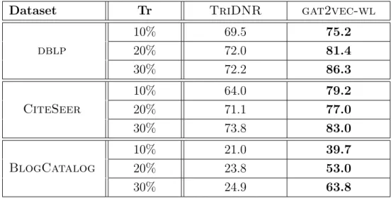
Various approaches have been proposed that use deep neural networks to learn an embedding jointly from network structure and the attributes [46– 53]. _TriDNR is a semi-supervised approach which uses network structure, network attributes and partial labels to learn an embedding [48]. It em-ploys a coupled model - one model exploits the inter-node relationships by using _SkipGram on network structure, other one exploits vertex-node and label-word relationships by using _Doc2Vec on node attributes and labels. The model uses a late fusion approach, i.e. the learning is per-formed independent of each other and the final embedding is obtained by a linear combination on two embeddings. The drawback with this approach

(47)

is that two different sources of information (structure and attributes) do not complement each other in learning. Another semi-supervised approach called Predictive Text Analytics (PTE) originally designed for text net-works, can also be used for graphs with attributes [46]. The word-word,

word-document, and word-label networks described in PTE can be trans-lated to node-node, node-attributes, and node-label networks for attributed graphs.

Graph Convolutional Network (GCN) based approaches have also been proposed for attributed graphs. Kipf and Welling proposed a fast and scalable semi-supervised approach that uses first-order approximations of spectral graph convolutions [53]. This approach is transductive, i.e. trains on network structure, thus the model cannot generalize to unseen nodes. An inductive approach called GraphSAGE uses node features for training and generated embedding for the vertices [2]. The model trains a set ag-gregator functions that aggregate information from nodes at a given depth from the current node. Thus, each node is represented by the aggregation of its neighbors. The paper proposed three aggregation functions: mean aggregator, LSTM aggregator and pooling aggregator. This process is done iteratively fork steps and at each step, the latent representation is updated as per aggregator functions.

Graph autoencoder has also shown promising results in learning an em-bedding using GCN [52, 54]. Variational Graph Autoencoder (VGAE)[52] is an unsupervised approach which uses GCN encoder and a simple inner product decoder.

Gao et al. pointed out that not only network structures are highly non-linear, but also the attributes of the network are non-linear as well [49]. Therefore, they proposed Deep Attributed Network Embedding (_dane), which employs a deep autoencoder on both the structure and the attributes simultaneously. The proposed approach preserves the first-order proximity

(48)

4.2. HETEROGENEOUS NETWORK EMBEDDING 32

in the network structure and the attributes, and the high-order proximity in the network structure only. Furthermore, the model maintains the con-sistency between two modalities, and a complementary representation is obtained by jointly optimizing on the joint distribution of two modalities. This requires sampling the vertices which are similar in attributes. The sampling strategy is quadratic which limits the scalability of DANE. An-other approach, ANRL uses an enhanced deep autoencoder which preserves structural proximities and attributes affinities [50]. The model takes only attributes as input and reconstructs the attributes and neighborhood of the given node. The neighborhood reconstruction is optimized against ground truth which is prior generated through random walks. Most of the ap-proaches only learn the representation of the nodes and not the attributes. A recent model called Co-embedding Attributed Networks (CAN) learns an embedding of both nodes and the attributes and use them in applications such as user profiling [51]. CAN employs a variational autoencoder and captures the affinities between nodes and attributes by projecting them in the same semantic space [55].

4.2 Heterogeneous Network Embedding

Some networks are by and large inherently heterogeneous. The NRL meth-ods designed for a homogeneous network cannot be directly used for these networks as these methods discard the node and edge types and the learned embedding cannot preserve the properties of such a network. On this ac-count, various approaches have been proposed [56, 56, 57, 57–60]. Yuxio et al. proposed _Metapath2Vec, which uses meta-path based random walks to generate the heterogeneous neighborhood contexts [56] and introduced heterogeneous _SkipGram model to learn an embedding. The meta-path based random walk uses a meta-path scheme which guides a random walker

(49)

to choose the next node in the walk, such that the semantics and structural correlations between different types of nodes are captured. The heteroge-neous _SkipGram model maximizes the probability of a node in hetero-geneous contexts and for efficient optimization, it uses negative sampling approach [61]. In an extension approach called _{Metapath2Vec++}, they use heterogeneous negative sampling which normalizes the softmax func-tion with respect to the node type of the context. _Hin2Vec is another meta-path based approach which learns the node representations as well as representations of the targeted relationships that are used to predict the target relationships between two nodes [58]. _Hin2Vec is a single layer, feed-forward neural network that takes 3 inputs- two nodes and the re-lationship between them - and trains a binary classifier which predicts whether the two input nodes have a specific relationship or not. The cum-bersome task is to sample the training data such that it covers as many node pairs and their relationships as possible. Moreover, the binary clas-sifier also requires negative samples which are populated by replacing one of the nodes in the input data tuple. The problem with the meta-path based approach is that it requires a user to define the schema to guide random walks, and second, these approaches require a very large number of walks for adequate sampling. To overcome these drawbacks, Rana et al. proposed a Jump and Stay strategy to perform random walks which not only performs better with meta-path based learning methods but also speeds up the learning [62].

A deep network approaches Heterogeneous Network Embedding (HNE) considers a heterogeneous network having different types of nodes and con-tents such as images, text [57]. Thus leading to a network in which we can have text-text links, image-image links, and image-text links. Thus, HNE strives to learn a unified embedding which preserves the content and rela-tional information. The neural network of HNE consists of three modules:

(50)

4.2. HETEROGENEOUS NETWORK EMBEDDING 34

image-image, image-text, and text-text which are fed with pairwise data from the _HIN. The image-image module employs a Convolutional Neural Network (CNN) for each image, image-text employs a CNN for image and Fully Connected (FC) layers for text, and FC layers for each text data input in text-text module. The weights are shared within and between the modules, and components are optimized through Stochastic Gradient Descent (SGC) for learning a unified embedding.

(51)

Chapter 5 Joint Learning on Attributed Graphs

The objective of network representation learning is to embed vertices in a low-dimensional space where the graph properties such as pairwise rela-tionships between vertices and the structure of vertex local neighborhood are preserved. The properties between vertices can be captured through local information (e.g. followers, citations, friendship relations) or global information (e.g. h-hop neighborhood, community affiliation). The sim-ilarity of a vertex with respect to other vertices represents its contextual information. The contexts obtained using structural information of the network are called structural contexts.

Similarly to structural contexts, we can define the context of vertices in terms of attributes. The contextual information based on attributes defines the semantic relationship between vertices. For example, in a citation network, two papers having similar keywords share contextual information irrespective of their distance in structure. It is a challenging task, however, to generate attribute contexts from attributed graphs, in particular when the coverage of attributes is only partial, as in Figure 5.1. The labels of vertices are used in the classification task.

In this chapter, we introduce _gat2vec, a framework that jointly learns from both the structure and the attributes of the network using a single

(52)

36

Figure 5.1: An example of a partially attributed graph.

neural layer. Structural contexts are obtained from the graph, preserving structural proximities; attribute contexts are obtained from a bipartite graph linking vertices and their attributes, preserving content proximities. The proposed framework learns a representation in an unsupervised manner, scaling to large graphs, for both directed and undirected homo-geneous graphs. Our approach is novel as it leverages multiple sources of information through early fusion and needs to optimize a single objec-tive function. Furthermore, we will present a semi-supervised variant of

gat2vec calledgat2vec-wl, where labels are incorporated as attributes

to enhance the learning of embeddings.

We empirically evaluated and validated our approach on vertex classi-fication (multi-class & multi-label) and link prediction, on real-world at-tributed networks. The qualitative analysis from visualization and query task also validates our approach.

(53)

37 CHAPTER 5. JOINT LEARNING ON ATTRIBUTED GRAPHS

the motivation and formally describe the problem. In Section 5.2, we present our proposed framework _gat2vec. We describe the experimental setup and experimental results in Section 5.3.

5.1 Problem

We investigate the problem of integrating structural and attribute con-textual information obtained from a partially attributed graph and employ a neural network model to jointly learn a representation of the vertices in a low-dimensional space. Informally, the problem can be described as fol-lows:

Problem Given an attributed graph G as shown in Figure 5.1, we aim at learning a low-dimensional network representation Φ : V → _Rd_{, where}

d |V| is the dimension of the learned representation, such that the structural and attribute contextual informations are preserved.

The learned representation Φ is generic and can provide feature inputs for various machine learning tasks, such as classification and link predic-tion. Its validity is evaluated through such machine learning tasks; the precise figures of merit to be used are described in the respective Sec-tions 5.3.4 and 5.3.5. For example, if the learned representation is able to classify vertices with high precision and recall (combined as F1 score), that means that the contextual information of vertices is well-preserved.

In this work, we considerGas a homogeneous, un-weighted and partially attributed graph. We evaluate our proposed approach on classification of vertices (multi-class and multi-label) and link prediction. We also perform a qualitative analysis (nearest-neighbor search and visualization).

(54)

5.2. GAT2VEC FRAMEWORK 38

Figure 5.2: A graph depicting the structural relationships between vertices.

5.2 GAT2VEC Framework

In this section, we present a detailed description of our proposed frame-work _gat2vec1 which learns a network embedding from structural and at-tribute information. For each vertex, we obtain its structural and atat-tribute contexts with respect to other vertices through random walks. Then, we integrate these two contexts to learn an embedding which preserves both structural and attribute proximities. The _gat2vec method is outlined in Algorithm 1. Specifically, our framework consists of three stages:

• Network generation

• Random walks

• Representation learning

5.2.1 Network Generation

From the attributed graph, G, we obtain two graphs:

(1) A connected structural graph Gs = (Vs, E), consisting of a subset

Vs ⊆ V of vertices that have connections included in the set E of

edges. We refer to vertices in Vs as structural vertices. An edge

1

(55)

(ps, qs) ∈ E encodes a structural relationship between nodes as shown

in Figure 5.2.

(2) A bipartite graph Ga = (Va,A, Ea), consisting of (i) the subset of

con-tent vertices Va ⊆V that are associated with attributes, (ii) the set of

possible attribute vertices _A derived from Z as given in the Definition 1 in Section 2.2 of Chapter 2, and (iii) the set of edges Ea

connect-ing content vertices to the attribute vertices that are associated by function A:

Va = {v : A(v) 6= ∅}

Ea = {(v, a) : a ∈ A(v)}

Figure 5.3: A bipartite graph between content nodes and attributes.

Proposition 1. Two content vertices u, v ∈ Ga are reachable only via

attribute vertices.

Following Proposition 1, the path between content vertices contains both content and attribute vertices. Therefore, the content vertices con-tained in the path have a contextual relationship because they are reach-able via some attribute vertices. These content vertices form the attribute

(56)

5.2. GAT2VEC FRAMEWORK 40

contexts. The intuition behind our approach is “two entities are similar, if they are connected with similar objects”. This phenomenon can be ob-served in many applications, e.g. in the bipartite “user-product” graphs, where “users” buy “products” and two users are similar if they buy similar products.

Such bipartite network structure has also been used in [46] which models a network between documents and the words included in them.

5.2.2 Random Walks

Informally speaking, similarity between entities could be measured in sev-eral ways. For example, it could be measured based on the distance of two nodes in the graphs. In the attributed graph of Figure 5.3, e.g., nodes 2 and 8 are both one attribute away from node 1, and thus we could say that they have equal similarity to 1; but there three paths connecting 1 and 8, while there are only two paths connecting 1 and 2; thus, 1 and 8 are more similar than 1 and 2.

While several approaches have been used [9, 26–28, 48], we adopt short random walks to obtain both the structural and the attribute contexts of vertices at the same time. The short random walks enable to effectively capture the contexts in which nodes have high similarity [26].

Random walks are performed on both Gs and Ga. The random walks

over Gs capture the structural context. For each vertex, γs random walks of

length λs are conducted to build a corpus R. This contextual information

is used in the embedding, with the aim of maintaining the local and global structure information. We denote ri as the i-th vertex in the random walk

sequence r ∈ R.

For example, a random walk in the graph of Figure 5.2 could be the following: r = (2,3,4,3,1), with length length 5, starting at vertex 2 and ending at vertex 1.

(57)

In the bipartite graph Ga, a random walk starts with a content vertex

and jumps to other content vertices via attribute nodes. The attribute vertices act as bridges between content vertices and help in determining the contextual relationships among them, i.e. which content vertices are closely related. As we are interested in how often such vertices co-occur in random walks and not in which attributes have been traversed to connect them, we have omitted the attributes in our random walks. Thus, the walks contain only vertices from Va.

Group of vertices that have high similarity in attributes are likely to appear frequently together in the random walks. Similar toGs, we perform

γa random walks of length λa and build a corpus W; we denote with wj

the j-th vertex of the random walk sequence w ∈ W.

For example, a random walk with attributes in the graph of Figure 5.3 could be the following: [2, b,1, c,8, b,2, b,8]. Since we are skipping attribute nodes in walks, therefore the corresponding walk is w = [2,1,8,2,8], with length 5, starting from vertex 2 and terminating in vertex 8.

5.2.3 Representation Learning